Abstract
With the development of Internet of Things and artificial intelligence, large amounts of data exist in our daily life. In view of the limitations in current data security risk assessment research, this paper puts forward an intelligent data security risk assessment method based on an attention mechanism that spans the entire data lifecycle. The initial step involves formulating a security-risk evaluation index that spans all phases of the data lifecycle. By constructing a symmetric mapping of subjective and objective weights using the Analytic Hierarchy Process (AHP) and the Entropy Weight Method (EWM), both expert judgment and objective data are comprehensively considered to scientifically determine the weights of various risk indicators, thereby enhancing the rationality and objectivity of the assessment framework. Next, the fuzzy comprehensive evaluation method is used to label the risk level of the data, providing an essential basis for subsequent model training. Finally, leveraging the structurally symmetric attention mechanism, we design and train a neural network model for data security risk assessment, enabling automatic capture of complex features and nonlinear correlations within the data for more precise and accurate risk evaluations. The proposed risk assessment approach embodies symmetry in both the determination of indicator weights and the design of the neural network architecture. Experimental results indicate that our proposed method achieves high assessment accuracy and stability, effectively adapts to data security risk environments, and offers a feasible intelligent decision aid tool for data security management.
1. Introduction
Data represent facts and observations and serve as a foundational element in digital systems. As a new type of production factor, data form the foundation of digitalization, networking, and intelligence. Data are rapidly permeating into various stages of production, circulation, consumption, and social service management, profoundly influencing and transforming human production methods, lifestyles, and governance models. With the advancement of information and digital technologies, data resources have grown at an unprecedented rate and are widely applied, providing strong momentum for social progress and economic growth, thereby highlighting the core position of data. Globally, the digital economy has become a driving force for continuous economic development [1]. As the digital economy’s contribution to national GDP has risen steadily in recent years, developed and emerging economies alike have made digital transformation a strategic priority. In the coming years, the digital economy is expected to continue its rapid growth, with its transformation being significantly driven by the proliferation of advanced AI models [2], including ChatGPT and DeepSeek.
However, data security is shifting from a peripheral issue to a strategic core, and it has become a critical factor in the development of the digital economy [3]. Data security entails implementing measures to protect data from illegal admission, corruption, or theft throughout their lifecycle, thereby ensuring thei confidentiality, integrity, and availability. As data become a central production asset in the digital economy, their associated security challenges have grown more complex, requiring the development of robust governance systems to address these complexities.
In practical production and daily life, data security risks mainly arise from human factors, technical vulnerabilities, and other reasons. During processes such as data collection, storage and usage, irregular handling activities and inadequate or absent security measures may compromise data integrity, confidentiality, and availability and trigger events such as information leaks, losses, and unauthorized use [4]. For example, gas data security risks directly impact the safety of the gas system, potentially leading to system failures or operational anomalies, which in turn may trigger a series of safety incidents such as leaks or explosions. In severe cases, this not only endangers human life but can also result in substantial property damage and environmental pollution. These data security incidents not only inflict immediate financial damage but can also jeopardize national security, potentially leading to catastrophic outcomes that erode national interests, societal well-being, and the lawful entitlements of both institutions and individual citizens. Therefore, it is crucial to conduct data security risk assessments [5].
Serving as a fundamental activity in data security and a pivotal element of data governance, data security risk assessment systematically scrutinizes the prevailing landscape of security threats, thereby furnishing sound, evidence-based guidance for safeguarding data and promoting its efficient utilization [6]. Through effective data security risk assessments of systems (institutions or organizations), risks can be scientifically quantified and categorized, determining their severity. This helps decision makers to prioritize risk management and determine the level of governance required. Additionally, it provides scientific evidence with which to guide the development of data security strategies, resource allocation, and the implementation of security measures. This ensures the effectiveness of security investments and enhances the system’s capability to identify, analyze, and respond to security risks, ultimately improving its overall protective capacity.
Based on the above circumstances, as a key component in the production and daily procedure of the digital economy era, data require the development of a risk assessment plan that covers their entire lifecycle, from collection, transmission, storage, processing, and exchange, to destruction. This plan should accurately assess and effectively manage data security risks, improve data security governance, and ensure that data are transferred and utilized securely, efficiently, and reliably within the digital economy. However, existing data security risk assessment methods largely rely on traditional information system security evaluation approaches and still lack dedicated frameworks that comprehensively address the entire data lifecycle. Furthermore, current practices suffer from the absence of a unified and systematic set of assessment indicators, with indicator weighting often determined based on subjective experience or a single method.
In response to these challenges, this study proposes a novel data security risk assessment method that covers the full data lifecycle. The proposed approach establishes a general indicator system for data lifecycle security risk assessment, integrates both the Analytic Hierarchy Process and the Entropy Weight Method to enable multidimensional weighting, and employs a fuzzy comprehensive evaluation method to label training data. The neural network model based on a bidirectional row–column attention mechanism is then adopted for training, achieving a risk assessment accuracy of over 97%. The method demonstrates high accuracy and stability, effectively adapting to dynamic data security risk environments. It offers a practical and intelligent decision support tool for enhancing data security management.
2. Related Works
With the swift evolution of the digital economy, data assets have been extensively leveraged across diverse industrial sectors. Data security risk assessment has attracted significant attention from administrative and business regulators. The related work of data security risk assessment research started early. Bethlehem J G et al. [7] addressed data leakage issues in 1990, explaining their real-world risks and proposing a theoretical approach based on the concept of uniqueness to aid in assessing data security risks. Currently, three principal approaches are employed to evaluate data security risks, detailed as follows.
(1) Qualitative data security risk assessment methods: Qualitative approaches to data security risk assessment, such as the Delphi technique [8], mainly rely on the assessors‘ experience, knowledge, and professional skills. These methods are highly subjective and require assessors to have a strong level of expertise and judgment.
(2) Quantitative data security risk assessment methods: Quantitative approaches involve measuring and analyzing risks through quantifiable indicators to enhance objectivity and comparability. Typical quantitative methods include clustering analysis [9], risk mapping, and Decision Tree analysis [10].
(3) Integrated qualitative and quantitative data security risk assessment methods: These methods combine the comprehensiveness of qualitative analysis with the objectivity of quantitative analysis, effectively improving the accuracy of risk assessments. They are widely applied in assessing risks within complex information systems.
Both the domestic and international literature largely rely on the three methods previously described and can be classified into two principal types, as detailed below.
2.1. Traditional Methods of Assessing Data Security Risks
Traditional data security risk assessment approaches largely rely on conventional theoretical models and expert experience. These methods typically involve constructing indicator systems, formulating risk assessment procedures, and employing techniques such as statistical analysis and fuzzy mathematics to stratify, quantify, and infer risks. They are suited for scenarios in which data volumes are relatively small and the environment remains stable.
Munodawafa F et al. [11] assessed the overall impact of data security risks in hybrid data center architectures using the EBIOS (Expression des Besoins et Identification des Objectifs de Sécurité) risk analysis method. Aiming at the diversity and complexity of data in intelligent connected vehicles, L. Wang et al. [12] built a data security classification framework from the aspects of vehicle data, personal data, and external environment data. Similarly, D. Liu et al. [13] proposed a theoretical framework for a full lifecycle data security risk analysis—encompassing data collection, storage, transmission, and usage—in the context of automotive data security. S. Zhou et al. [14] examined the data security challenges in intelligent connected vehicles through the exploration of security reverse engineering techniques, proposing a model for assessing data security potential and calculating the associated security risk values. In the field of gas data security risk assessment, Z. Ba et al. [15] used an improved Analytic Hierarchy Process to determine indicator weights, then proposed a fuzzy comprehensive evaluation to construct a gas pipeline risk assessment model. By using an experience-driven risk assessment method, Melgarejo Diaz N et al. [16] developed an information security management system that corresponds to the enterprise risk management framework. Alvim M S et al. [17] introduced a privacy analysis method based on Quantitative Information Flow (QIF), which can accurately calculate the privacy leakage risk of datasets under various attack scenarios. Alonge C Y et al. [18] proposed a fuzzy logic-based framework for the classification and identification of data and information assets. To enhance classification accuracy and concordance, this framework combines fuzzy logic with the Delphi method for security risk assessment. To ensure the integrity and availability of critical data, S. S. Hussaini et al. [19] put forward an integrated risk assessment model by adopting a dynamic, iterative evaluation framework that continuously optimizes risk identification and defense capabilities. Hossain N et al. [20] put forward a risk assessment methodology that integrates system analysis, attack modeling and evaluation, and penetration testing to demonstrate the effects of attacks on system security. With the assistance of security experts, Ron Bitton et al. [21] utilized the NIST enterprise network cybersecurity risk assessment framework and applied the Analytic Hierarchy Process to rank various attack attributes, thereby enabling security practitioners to accurately assess and compare the risks associated with different attacks.
2.2. Intelligent Methods of Assessing Data Security Risks
Based on traditional methods, intelligent data security risk assessment techniques utilize large volumes of historical data to automatically identify risk characteristics and correlation patterns. These techniques enable adaptive modeling and prediction of data-related risks. Common algorithms include neural networks, Decision Trees, and Support Vector Machines, which are particularly effective in addressing the challenges of large data volumes, complex environments, and dynamic changes. These approaches improve both the accuracy and timeliness of risk assessment results.
Siami M et al. [6] proposed an autonomous fuzzy decision support system for risk assessment. This system combines advanced artificial intelligence, unsupervised learning, and fuzzy logic to learn from uncertain and unlabeled big data for maximum utility. In response to the high sensitivity and privacy concerns of healthcare data, X. Zhang et al. [22] introduced a privacy risk assessment model that integrates information entropy and the fuzzy C-means clustering algorithm. Y. Bai et al. [23] proposed a novel data risk assessment model integrating a Knowledge Graph, a Decision-Making Trial and Evaluation Laboratory, and a Bayesian network (BN) to analyze gas pipeline accidents in a data-driven way in order to minimize the reliance on experts of the current BN-based approach. X. Zhang et al. [24] proposed a series of security assessment methods with data stream analysis and machine learning to address the increasing threats of data leakage and damage; their scheme also proves the feasibility of the security risk evaluation method based on machine learning. For risk assessment of cyberspace data assets, C. Meng et al. [25] developed a neural network-based method, which aims to solve the problems of long assessment period, low accuracy, and incomplete data in traditional assessment methods. Huang B et al. [26] studied the application of machine learning technology in enterprise risk assessment, and implemented three machine learning algorithms to evaluate various data security risks within enterprises. Muhammad A H et al. [27] applied Support Vector Machine, Random Forest, and gradient boosting algorithms to classify and predict information security risk assessment data. This methodology enables small and medium-sized enterprises to receive rapid, cost-efficient, and tailored risk assessments.
In recent years, the attention mechanism [28] has been widely adopted in various security risk assessment scenarios due to its high efficiency in capturing correlations between features. For instance, to address over-reliance on expert judgment in the cybersecurity situation assessments of modern power systems, S. Yong et al. [29] proposed a data fusion situation assessment method based on the attention mechanism, where the evaluation task is performed by deep neural networks. This approach achieves expert-level accuracy while significantly reducing manual intervention. In the context of security threats to industrial control equipment and network systems, Y. Liu et al. [30] combined self-attention mechanisms with Long Short-Term Memory (LSTM) neural networks to analyze time-series data for security situation prediction, thereby improving assessment accuracy. Their method outperformed traditional algorithms such as Random Forests, Support Vector Machines, and K-Nearest Neighbors. To enhance the defense capability against various types of cyberattacks, Chen J. et al. [31] innovatively integrated a multi-head attention mechanism with a gated recurrent unit (GRU). The improved multi-head attention enables the extraction of security features from different positions, enhancing the model’s learning ability in cybersecurity risk prediction and supporting network security situation assessment. In the financial domain, Xiao X. et al. [32] integrated bidirectional LSTM networks with a multi-head attention mechanism to capture complex temporal dependencies in payment patterns. They constructed a comprehensive risk assessment framework for detecting anomalous payment behaviors of small and medium-sized enterprises and predicting financial risks. Additionally, C. Chen et al. [33] proposed a threat assessment method based on a self-attention and GRU hybrid model to address aerial threats in modern air combat scenarios. Despite these advances, research on applying an attention mechanism specifically to data security risk assessment remains limited, highlighting the need for further in-depth exploration and practical implementation in this domain.
Grounded in the preceding review of data security risk assessment approaches both domestically and internationally, although research in the field of data security risk assessment has seen some progress, there are still the following problems.
(1) Most existing data security risk assessment models are still grounded in traditional information system risk assessment frameworks. These models primarily focus on the security of entire information systems, and there is still a lack of relevant research on the security risk of the data itself, especially the evaluation of the whole lifecycle of data, so it is urgent that we carry out in-depth discussion and practical work in this field.
(2) At present, all kinds of data security risk assessment schemes lack an objective and specific indicator framework for assessing data security risks. Most existing indicator systems are developed within the context of specific fields without specifically addressing the risks inherent to the data itself. Moreover, these systems lack uniform standards and theoretical foundations in terms of evaluation perspectives and indicator definitions.
(3) In existing models, the assignment of indicator weights often lacks a combination of subjective and objective justification. Consequently, these systems do not accurately reflect the true risk correlations and relative importance among the indicators, which undermines the credibility and persuasiveness of the assessment results.
In order to tackle these challenges, this paper proposes an intelligent data security risk assessment scheme based on an attention mechanism, adopting an integrated qualitative and quantitative approach. The main contributions of our scheme are as follows.
(1) A universal indicator system for data security risk assessment covering the entire data lifecycle: The proposed indicator system is closely aligned with diverse data flow scenarios and systematically covers the entire process from data collection to destruction, thereby ensuring a comprehensive risk assessment.
(2) Multidimensional indicator weight allocation: Unlike traditional risk assessment methods, which often use simplified approaches (such as equal weighting) for indicator weights, our proposed scheme employs a combination of the Analytic Hierarchy Process and the Entropy Weight Method. The AHP method provides a subjective evaluation by having specialist score the significance of each indicator, while the EVM objectively calculates the information entropy of each indicator based on the properties of the data. This combined approach effectively considers both expert judgment and data characteristics, ensuring a comprehensive and accurate allocation of indicator weights.
(3) A neural network model for data security risk assessment based on an attention mechanism: We use a fuzzy comprehensive evaluation method to evaluate data security risks, and the result is used as the risk grade label. Then, the labeled dataset is constructed as the input of the neural network. Through the training of an attention-based neural network, the model realizes automatic extraction and deep learning of multidimensional features of input data. Compared with traditional methods, this approach can capture complex patterns and nonlinear associations within the data, resulting in more precise and accurate risk assessments with an accuracy rate of over 97%. Additionally, with continuous learning and iteration, the neural network model is able to update its parameters in response to changing data, thereby maintaining high real-time performance and flexibility in practical applications and accommodating the continually evolving risk environment.
The remainder of this paper is divided as follows: Section 3 mainly introduces the main technical knowledge points involved in this solution. Section 4 introduces in detail the intelligent data risk assessment solution designed in this paper, including indicator system construction, indicator weight determination, the risk assessment model, etc. Section 5 details experiments conducted on specific data security risk assessment scenarios and compares them with other solutions. Section 6 summarizes this solution and elaborates on future research prospects.
3. Preliminaries
This chapter mainly explains the relevant basic theories involved in this scheme in detail.
3.1. Attention Mechanism
With the advancement of machine learning algorithms, methods such as the Latent Dirichlet Allocation (LDA) algorithm [34], Naive Bayes algorithm [35], and Decision Tree algorithm [36] have been widely applied in various scenarios. The attention mechanism has emerged in recent years as a rapidly developing technique in deep learning. The core idea of the attention mechanism is to mimic the human cognitive ability to selectively focus on critical information. This mechanism dynamically adjusts the neural network’s focus on input features through a parameterized weight matrix, enabling the model to autonomously identify regions with high information content and perform adaptive feature selection accordingly. Essentially, for each input query, the attention mechanism works by selectively “attending” to different keys and then performing a weighted aggregation of the values corresponding to these keys to obtain the most relevant information.
The various forms of attention mechanisms generally include self-attention, multi-head attention, masked self-attention, and cross-attention. The following mainly introduces the self-attention and multi-head attention mechanisms.
3.1.1. Self-Attention Mechanism
The self-attention mechanism overcomes the limitations of traditional sequence modeling. It builds a fully connected network within the input sequence to enable dynamic interactions between elements at any position. Specifically, this mechanism employs the triple projection system of Query, Key, and Value to mathematically model the input sequence as follows.
(1) Linear transformation: For the input , three distinct linear transformations are applied to generate the Query , Key , and Value matrices. Specifically, , , and represent the mappings for Query, Key, and Value, respectively:
where , , and are weight matrices, as shown in Figure 1.
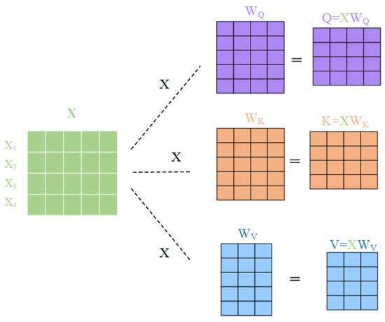
Figure 1.
Linear transformation process in the self-attention mechanism.
(2) Calculation of attention weights: The attention weights are calculated from the Query and Key . Their relationship is given by
Figure 2 shows the computation procedure of the attention weights in the self-attention mechanism. The result is a matrix that represents the similarity between each query position and all other key positions.
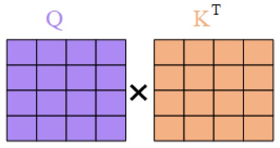
Figure 2.
The calculation process of attention weight in the self-attention mechanism.
(3) Scaling: To avoid excessively large values, it is necessary to scale the similarity by the factor , where is the scaling factor, usually the vector dimension of the Query or Key. This is used to prevent the dot product from becoming excessively large, which could lead to gradient instability. The scaling process is shown in Figure 3.
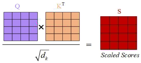
Figure 3.
The scaling procedure in the self-attention mechanism.
(4) Normalization: The Softmax function is applied to the scaled score to normalize the dot product score to the interval (0,1), thus obtaining the attention weight vector. Figure 4 shows the normalization process.
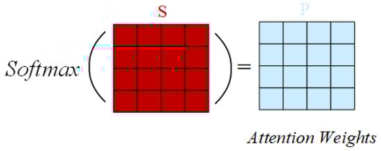
Figure 4.
Normalization process in the self-attention mechanism.
(5) Weighted sum: Eventually, the obtained attention weights are used to compute a weighted sum with the value matrix , resulting in the final representation at each position. The following formula is the classic scaling dot product attention formula. Figure 5 illustrates the process of weighted summation.
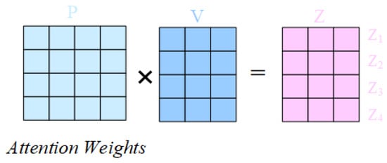
Figure 5.
Weighted sum process in the self-attention mechanism.
The whole process is shown in Figure 6.
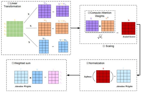
Figure 6.
The full workflow of the self-attention mechanism.
The self-attention mechanism has the benefit of allowing each position to consider information from all other positions, allowing it to capture long-range dependencies. Unlike traditional methods such as RNN, the self-attention mechanism does not rely on the sequential order of inputs, making parallel computation possible.
3.1.2. Multi-Head Attention Mechanism
The standard self-attention mechanism can only learn a single “mapping relationship”, which might be limited to one subspace or attention pattern. The multi-head attention mechanism is an extension of self-attention that improves the model’s representational capacity by allowing it to learn from different feature subspaces through multiple attention heads. In multi-head attention, the input vectors , and are first split along the feature dimension into several sub-blocks (heads). Each head performs attention operations independently, and their outputs are then concatenated. This enables the model to capture various types of relationships or interactions in parallel from different perspectives.
Figure 7 shows the computation process of multi-head attention; the specific description is as follows.
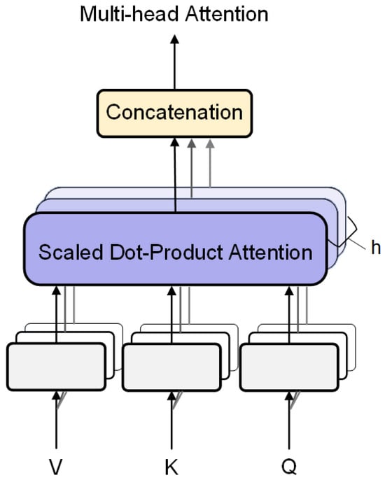
Figure 7.
Model based on the attention mechanism.
(1) Mapping of the input to multiple heads, where each head independently performs self-attention computation:
(2) Concatenation and linear transformation:
where h denotes the number of heads, and is the output linear transformation matrix.
3.2. Multilayer Perceptron
In attention-based networks, a fully connected neural network is often employed after the attention module to enhance nonlinear representation capabilities. The fully connected neural network—commonly called a multilayer perceptron (MLP)—represents one of the foundational and central architectural frameworks in neural network architectures. Its essential mechanism involves stacking fully connected layers with nonlinear activation functions to construct high-level feature abstraction from input to output. The primary objective of an MLP is to perform complex nonlinear transformations on data through multiple fully connected neuron layers, thereby establishing a mapping relationship between input features and output labels. It is commonly applied in supervised learning tasks such as classification and regression.
The fundamental structure of an MLP comprises an input layer, one or more hidden layers, and an output layer. The overall structure is shown in Figure 8.
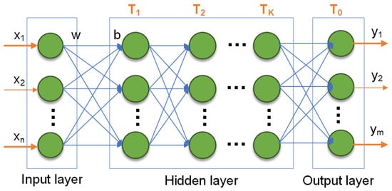
Figure 8.
The structure of the MLP.
(1) Input layer: Input data are fed into the network such that each neuron corresponds to a specific input feature.
(2) Hidden layer: Each hidden layer contains many neurons, each of which is fully connected to all neurons in the preceding layer to facilitate feature extraction.
(3) Output layer: The output layer produces the final output. The number of neurons in this layer is determined by the task type. For classification, the output layer neuron count equals the number of classes, and a Softmax activation function is typically used to generate class probability distributions. For regression, the output layer usually contains a single neuron that directly yields the predicted value, with a linear activation function commonly applied. Common activation functions include Sigmoid, ReLU, and Softmax.
The computational formula for each layer is as follows:
where is the input to the layer; is the weight matrix of the layer; is the bias term of the layer; and T is the activation function of the layer.
3.3. Residual Connection and Layer Normalization
As shown in Figure 9, in attention-based models, residual connections and layer normalization are two crucial components that operate jointly across various layers of the network to enhance both training efficiency and model performance.
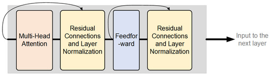
Figure 9.
Model based on the attention mechanism.
As illustrated, in attention-based models (such as the Transformer architecture), each layer first processes self-attention or cross-attention mechanisms, followed by residual connections and layer normalization. Subsequently, feedforward neural network processing is applied, again followed by residual connections and layer normalization.
3.3.1. Residual Connection
Residual connections are employed to mitigate gradient vanishing and degradation problems in deep networks. The core approach involves the following steps. After each sub-layer’s (or several layers’) output, the input itself is added before subsequent processing, enabling the network to directly learn the difference between output and input, i.e., the so-called “residual”. The formulation is
where is the input to a sub-layer, and represents the nonlinear transformation of that layer.
Deep neural networks frequently experience vanishing or exploding gradients in training, but the addition of residual connections substantially alleviates this issue. By allowing gradients to propagate directly to earlier layers, the residual structure significantly improves the trainability of deep networks. Moreover, this structure enables the network to learn only the residual between input and output, rather than the complete mapping function, thereby reducing the difficulty of learning. Additionally, residual connections allow input information to be directly transmitted to deeper layers, virtually preventing the loss of critical information due to multiple nonlinear transformations.
3.3.2. Layer Normalization
Layer normalization is typically applied after residual connections. By normalizing the output of all neurons in the layer, the output distribution has a stable mean and variance. The processing flow of layer normalization is as follows:
(1) Computation of mean and variance: For any vector , calculate the mean and variance for all features:
(2) Normalize all features of the sample using the computed mean and variance:
where is a small constant to prevent division by zero.
(3) Learnable scaling and shifting:
where and are learnable parameters for scaling and shifting the normalized results. This approach maintains distribution stability while preserving flexibility.
4. Intelligent Risk Assessment Scheme
4.1. Risk Assessment Model
Data security risks are not limited to a single stage, for example, storage or transmission; instead, they extend throughout the entire lifecycle. Every stage—from data collection, transmission, storage, processing, and exchange to destruction—may be exposed to various security threats. Conducting a risk assessment across the entire data lifecycle allows for the comprehensive identification and estimation of potential risk levels, thereby making certain that appropriate security measures are requested at every stage. As illustrated in Figure 10, the data security risk assessment scheme proposed in this paper mainly consists of the following components:
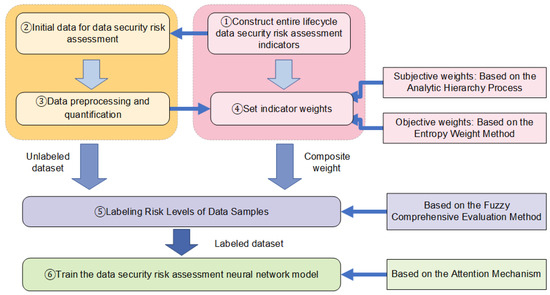
Figure 10.
Model diagram of data security risk assessment.
(1) Based on the distinct stages of the full data lifecycle, a comprehensive security risk assessment indicator system for the entire lifecycle is designed and established through a review of relevant literature and standards.
(2) Various logs and operational information related to the data under evaluation are collected to obtain initial sample data for a comprehensive security risk assessment of the entire data lifecycle. Subsequently, through data preprocessing and the quantification of the indicators determined in step (1), the final dataset for neural network training is derived.
(3) Based on the indicators obtained in step (1) and the dataset acquired in step (2), the comprehensive weight of each indicator is obtained by using AHP and EWM.
(4) Based on the comprehensive weights derived in step (3), the fuzzy comprehensive evaluation method is applied to label the risk levels of the dataset from step (2).
(5) A neural network for data security risk assessment, enhanced with an attention mechanism, is developed and trained on the labeled dataset from step (4).
4.2. Constructing Indicator System
This scheme establishes a universal indicator system for full lifecycle data security risk assessment, thereby ensuring its applicability to the vast majority of data security risk assessment scenarios.
4.2.1. Indicators for Risk Assessment of Data Collection Security
Data collection security is the primary stage of data security management. It is necessary to ensure that the confidentiality, integrity and availability of data are not threatened during data collection. Data collection constitutes the first and most critical step in the data lifecycle, as the data gathered may directly impact the subsequent security of data storage, processing, analysis, and utilization. The evaluation indicators for this stage are shown in Table 1.

Table 1.
Indicators for risk assessment of data collection security.
4.2.2. Indicators for Risk Assessment of Data Transmission Security
As an integral part of the data security lifecycle, data transmission security ensures protection against unauthorized access, tampering, and data loss during transfer. In this scheme, the evaluation indicators proposed in the data transmission stage are shown in Table 2.
Table 2.
Indicators for risk assessment of data transmission security.
4.2.3. Indicators for Risk Assessment of Data Storage Security
Data storage security refers to the protection of digitally stored information, focusing on maintaining data confidentiality and integrity through encryption and other measures. The evaluation indicators proposed in the data storage stage are shown in Table 3.
Table 3.
Indicators for risk assessment of data storage security.
4.2.4. Indicators for Risk Assessment of Data Processing Security
The main task of data processing security is to ensure that data are not leaked, tampered with, or misused during processing, while meeting compliance and privacy protection requirements. Data processing security requires the security of the original data integration, cleaning, conversion and other operational stages. The evaluation indicators proposed in the data processing stage are shown in Table 4.
Table 4.
Indicators for risk assessment of data processing security.
4.2.5. Indicators for Risk Assessment of Data Exchange Security
Data exchange security focuses on preventing data leakage, tampering, and unauthorized access during the exchange process. The evaluation indicators proposed in the data exchange stage are shown in Table 5.
Table 5.
Indicators for risk assessment of data exchange security.
4.2.6. Indicators for Risk Assessment of Data Destruction Security
Data destruction security represents the final phase in the management of the entire data lifecycle. Its goal is to ensure that data cannot be recovered after destruction through appropriate technical means and management measures, thereby preventing the leakage of sensitive information. The evaluation indicators for data destruction are shown in Table 6.
Table 6.
Indicators for risk assessment of data destruction security.
4.3. Determination of Indicator Weights
The data security risk assessment indicators for the entire data lifecycle proposed in this scheme are shown in Figure 11. As shown in the figure, a comprehensive data security risk assessment for the entire lifecycle encompasses 6 stages and a total of 30 indicators. This evaluation indicator set is represented as
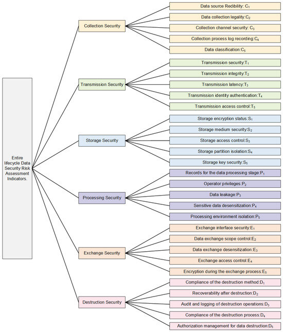
Figure 11.
Security risk assessment indicators throughout the entire data lifecycle.
However, in the risk assessment process, these 30 indicators do not contribute equal weight. Therefore, it is necessary to assess these indicator weights so that decision makers can allocate resources and formulate strategies accordingly. Moreover, when neural networks are subsequently employed for data security risk evaluation, these indicator weights will also impact the accuracy and rigor of the data assessment results.
Commonly used methods for determining subjective indicator weights include the Analytic Hierarchy Process, the Delphi method, and others. Among them, the Delphi method generally provides only a series of indicators without a systematic hierarchical decomposition, which may make it difficult for experts to form an overall understanding. Moreover, although the Delphi method gathers consensus through multiple rounds of anonymous questionnaires, it lacks a means to quantitatively verify the consistency of expert opinions. In contrast, the AHP allows for the decomposition of complex problems into layers and levels. Experts only need to perform pairwise comparisons among indicators within the same level, and consistency tests are used to ensure the logical reliability of judgments.
Commonly used methods for determining objective indicator weights include the Entropy Weight Method and the Criteria Importance Through Intercriteria Correlation (CRITIC) method. The CRITIC method, based on standard deviation and correlation, accounts for both the variability of indicators and the correlations between them, making it suitable for scenarios where indicators are strongly correlated. In contrast, the EWM calculates weights based solely on the distribution characteristics of the data, making it more suitable for situations with weakly correlated indicators. It can ensure that risk factors with a high degree of data dispersion receive higher weights without being disturbed by other indicators and are independent of the absolute size of the values.
Therefore, the overall approach of this study is to assign subjective weights to each indicator using the AHP based on expert evaluations and to derive objective weights using the EWM based on the actual data distribution. These subjective and objective weights are then combined into comprehensive weights through weighted fusion, thereby constructing a complete evaluation model.
4.3.1. Determining Subjective Weights Using the Analytic Hierarchy Process
The present scheme employs the following Analytic Hierarchy Process [37] to determine the subjective weights of the indicators. The primary step of the AHP is to set up a hierarchical structure model, which generally contains the goal layer, the indicator layer, and the alternative layer, as shown in Figure 12.
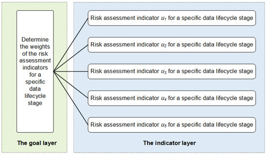
Figure 12.
The structure of determining the index weights based on the AHP.
In this scheme, two key considerations are taken into account: first, the impact of different stages of the data lifecycle on risk assessment results varies across scenarios, and second, matrix operations involve computational and storage challenges. We adopt a phased approach to determine weights and synthesize them in the final step. This method not only reflects the diverse impact of each lifecycle stage on the risk assessment results but also confines higher-order matrix operations and storage demands to lower levels. In this scheme, the process of determining subjective indicator weights based on the AHP is illustrated in Figure 13.
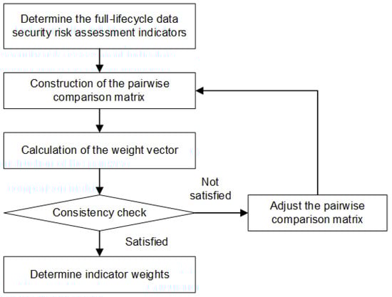
Figure 13.
The flowchart for determining subjective weights based on the AHP.
The details are as follows.
1. Construction of the pairwise comparison matrix
(1) Expert scoring
Assume there are K experts in the relevant field. Each expert compares every indicator for each period t (where , respectively, corresponding to the stage of data collection, transmission, storage, processing, exchange, and destruction) according to the pairwise comparison scale of the AHP, thereby constructing the pairwise comparison matrix (judgment matrix). The AHP pairwise comparison scale is defined in Table 7.
Table 7.
Explanation of the pairwise comparison scale values in the AHP.
K experts, drawing on domain knowledge and other relevant criteria, construct the pairwise judgment matrix according to the pairwise comparison scale of the AHP. The indicator judgment matrix of each period is as follows:
denotes the judgment matrix obtained by the k-th expert from pairwise comparisons of the five indicators within the t-th period.
(2) Construction of the Pairwise Comparison Matrix
The final pairwise comparison matrix for period t is obtained by integrating all K experts’ judgment matrices . The integration process employs the geometric mean method. Specifically, suppose that K experts provide scale values for a given element of the judgment matrix as (where ); then, the geometric mean of that element is given by
Then, the final judgment matrix of the t-th period is
where . At this point, there are only six judgment matrices for each cycle indicator, corresponding to the six cycles of the entire data lifecycle.
2. Calculation of the weight vector
For the indicator judgment matrix of the t-th stage, the steps to calculate the weight vector are as follows.
(1) Construction of the normalized matrix
At the t-th stage, the elements of the normalized matrix are computed by dividing the corresponding element from the original judgment matrix by the sum of its corresponding column. Specifically, the sum for each column j is calculated as follows:
The computation formula for each element of the normalized matrix is
The normalized matrix for the t-th stage is represented as
(2) Calculation of the weight vector
For the t-th stage, the weight of the i-th indicator is the average of the elements in the i-th row of the normalized matrix , calculated as follows:
where n is the order of the judgment matrix, i.e., there are n indicators. In this case, . Then, the weight vector for the t-th cycle indicators is given by
It satisfies the condition .
3. Consistency check
When constructing the judgment matrix, it is possible to make logical errors, so a consistency check is required to assess whether the matrix exhibits any inconsistencies. The steps for the consistency check are as follows.
(1) Calculate the maximum eigenvalue of the indicator judgment matrix for the t-th stage using the following formula:
(2) Calculate the consistency index using the following formula:
At this point, if , it indicates that there is complete consistency; if is close to 0, it indicates the satisfactory consistency. The larger the is, the more severe the inconsistency.
(3) Obtain the value by consulting the table. is the random consistency index, and it is related to the order of the judgment matrix. In general, as the order of the matrix increases, the probability of random consistency deviation also increases. Its values are provided in Table 8:
Table 8.
Correspondence between matrix order n and the value of .
(4) Calculate the consistency ratio . Considering that deviations in consistency may be due to random factors, when testing whether the judgment matrix exhibits acceptable consistency, the consistency index must be compared with the random consistency index . The test coefficient is calculated as follows:
If , the judgment matrix is considered to have passed the consistency check; otherwise, it does not exhibit satisfactory consistency. If the data do not pass the consistency check, it is necessary to check for logical issues and re-enter the judgment matrix for further analysis.
4. Calculation of the final entire lifecycle subjective indicator weights
Suppose the weights assigned by experts for each stage are as follows:
Here, corresponds to the weight for the t-th stage from data collection to destruction, and they satisfy the condition: .
For each stage, the indicator weight vector calculated using AHP is
Finally, the subjective indicator weight for the i-th indicator in the t-th stage of the entire data lifecycle is computed as:
4.3.2. Determining Objective Weights Using Entropy Weight Method
This scheme utilizes the Entropy Weight Method [38] to determine the objective indicator weights. The specific process is shown in Figure 14.
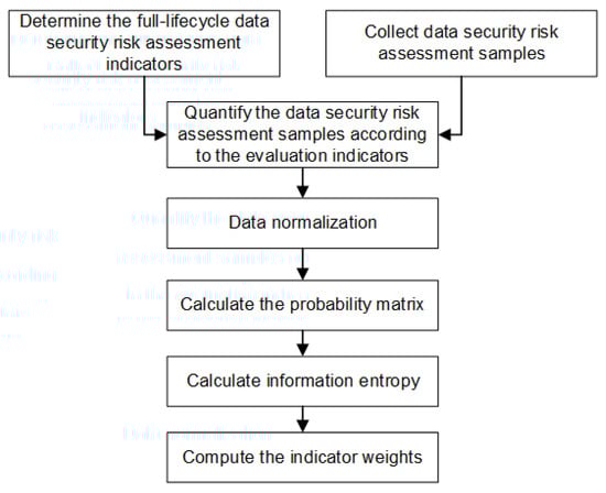
Figure 14.
The flowchart for determining the weights of objective indicators based on EWM.
Based on the risk assessment indicators of the entire data lifecycle established in this scheme, we collect and quantify N samples of data security risk assessment. The original data matrix is shown below.
where N is the number of data samples; n is the number of assessment indicators; and represents the value of the i-th sample for the j-th data security risk assessment indicator, with and .
1. Data normalization
Due to the differing value ranges among the risk assessment indicators, normalization is required to constrain their values between . A commonly used min–max normalization method is as follows:
(1) For extremely large indicators (i.e., higher values are better),
where is the maximum value for the j-th indicator and is the minimum value for the j-th indicator.
(2) For extremely small indicators (i.e., lower values are better),
Then, the normalized matrix is given by
2. Calculation of the probability matrix
For each element of matrix , calculate the probability distribution for each indicator. The formula for is given by
where represents the contribution rate of the i-th sample to the j-th data security risk assessment indicator. The probability matrix is given by
3. Calculation of information entropy
The information entropy of the j-th data security risk assessment indicator is calculated by the following formula:
where the normalization coefficient is defined as , ensuring that lies within the interval . Note that if , then is defined to be 0. The information entropy reflects the data distribution of the indicator.
(1) If is large, it indicates that the data distribution of the indicator is relatively uniform, providing less information, so the weight should be lower.
(2) If is small, it indicates that the values of the indicator vary more, providing more information, so the weight should be higher.
4. Calculation of the entropy weight
Based on , the information utility value is calculated as follows:
represents the contribution of the information of the j-th data security risk assessment indicator, i.e., the importance of that indicator.
Eventually, the entropy weight (the objective weight of the indicator) is calculated as follows:
4.3.3. Determining Comprehensive Weights of Indicators
Assume that for a certain security risk assessment indicator in the entire data lifecycle, the subjective weight obtained using AHP is , and the objective weight obtained using EWM is . Then, the composite weight for that indicator using the AHP–EWM combined weighting method is given by
where represents the balancing coefficient between the subjective and objective weights.
To obtain the optimal balancing coefficient , we adopt the least squares method to obtain the optimal . Its main principle is to minimize the sum of squared deviations between the composite weight and both the subjective weight and the objective weight , thereby obtaining the value of . It secures an optimal compromise in the composite weight between subjective preferences and objective data. The specific solution steps are as follows.
(1) Construction of the Objective Function:
In minimizing the squared error between the composite weight and both the subjective weight and the objective weight to define the objective function, the expression is as follows:
where n is the total number of indicators in the evaluation system.
(2) Differentiation with Respect to :
Take the derivative of the objective function with respect to . When the first derivative of the objective function is set to zero, the minimum of the squared error is obtained. In this case, we found that , meaning that the optimal balancing coefficient is 0.5, which indicates that the subjective weight and the objective weight are weighted equally. Thus, the composite weight using the combined AHP–Entropy Weight method is
This weight calculation method is applicable in scenarios where the subjective and objective weights are equally important. In practical applications, different values for may be set based on the actual situation to emphasize either the subjective or the objective weight. Finally, the complete set of entire data lifecycle risk assessment indicator weights is obtained as follows:
4.4. Annotation and Representation of the Dataset
4.4.1. Annotating the Dataset
In this scheme, we use the fuzzy comprehensive evaluation method to mark the risk assessment grade of the collected and quantified data samples. The detailed steps are as follows.
1. Determination of the evaluation indicator set
In the process of risk grade labeling for quantified data samples, we adopt the data lifecycle risk assessment index system U determined by this scheme as the evaluation index system.
2. Determination of the evaluation level set
In this scheme, the evaluation level set V is defined in three levels:
This level classification is used to assess the security risk level of data samples throughout their lifecycle and issubsequently employed in the fuzzy comprehensive evaluation calculations.
3. Determination of the evaluation indicator weights
The weights of the assessment indicators are the composite weights obtained using the combined weighting method of the AHP and the EWM:
where , and , which represents the number of indicators.
4. Construction of the fuzzy evaluation matrix
Each indicator is associated with a membership value for each evaluation level, reflecting the degree to which the evaluation object under that indicator belongs to a specific evaluation level. The matrix is typically constructed as
i.e., , where
(1) n represents the number of indicators, which is 30 in this scheme;
(2) m represents the number of evaluation levels, which is 3 in this scheme;
(3) represents the membership degree of the i-th indicator for the j=th evaluation level. The membership degree is typically obtained through expert judgment, survey, or statistical data analysis, and each indicator satisfies the condition ;
(4) Each row of the matrix represents the membership degree vector of a particular indicator for different risks. In this scheme, since the evaluation level set is divided into three levels, the membership function is defined as follows. For a given indicator ,
- When , the membership degree for high risk is 1, and the membership degrees for the other risks are 0;
- When , the membership degree for medium risk is 1, and the membership degrees for the other risks are 0;
- When , the membership degree for low risk is 1, and the membership degrees for the other risks are 0.
For example, regarding the credibility of data sources in data collection security, if its quantified value is 1, indicating low credibility, then its membership degree vector is ; if its quantified value is 2, indicating medium credibility, then its membership degree vector is ; and if its quantified value is 3, indicating high credibility, then its membership degree vector is .
Membership function is the link from “precise quantification” to “fuzzy calculation” and then to “quantitative output” in fuzzy comprehensive evaluation, and it plays a key role in effectively connecting objective data with the fuzzy evaluation model. In this scheme, the designed membership function is a mapping based on categories rather than on numerical magnitude. The core idea is that the membership degree only depends on the risk level to which the indicator belongs (low, medium, or high), regardless of the interval or magnitude of its specific quantification encoding values. Using this method, as long as the categorical semantics (“low”, “medium”, and “high”) remain unchanged, the membership matrix remains completely consistent, thereby ensuring that the final fuzzy evaluation vector is not affected by the quantification encoding method. The advantage of this design is that it eliminates the arbitrariness of numerical scales, removes human bias caused by different quantification intervals, and ensures that the evaluation results strictly reflect the categorical meaning of the indicators rather than numerical differences. At the same time, it maintains a high degree of simplicity and interpretability in the computation process and meets the fuzzy comprehensive evaluation requirement of “clear categorization to unique membership”, providing strong robustness and reproducibility for the indicator encoding scheme.
5. Calculation of fuzzy comprehensive evaluation
We calculate the comprehensive evaluation vector with the following formula:
where .
6. Annotation of the risk levels of the dataset
When labeling the dataset, based on the comprehensive evaluation vector , we select the risk level with the highest membership degree as the risk label for the data sample.
4.4.2. Representing the Dataset
For risk assessment over the entire data lifecycle, each data sample is evaluated using 30 indicators, and each sample may be assigned one of three risk labels through fuzzy comprehensive evaluation. Therefore, let denote the sample vector, where each dimension corresponds to the quantification value of a risk assessment indicator; let denote the risk category label (corresponding to low risk, medium risk, and high risk, respectively). Then, the data security risk assessment dataset containing N samples can be represented as
4.5. Data Security Risk Assessment Model
In this scheme, after labeling the initial dataset with risk levels through the fuzzy comprehensive evaluation method, we use an attention-based neural network model to train the collected risk assessment dataset. The characteristic vector of each training sample is composed of the quantification values of the risk assessment indicators, and its label is uniquely determined by the risk level using the fuzzy comprehensive evaluation method.
In order to fully leverage the dual information interactions in both the “indicator dimension” and “sample dimension” of the risk assessment dataset, this scheme constructs a data security risk assessment neural network model based on a row–column bidirectional attention mechanism [39] combined with a multilayer perceptron (MLP) to perform risk label prediction. The core of the model lies in capturing correlations among indicators within individual samples using intra-row attention and capturing distribution patterns of the same indicator across different samples using intra-column attention, further enhanced by an MLP sub-layer for nonlinear representation and fusion. The main steps of the procedure are as follows:
(1) Apply intra-row attention on the 30 indicators of a single sample to capture the correlations among the indicators within that sample.
(2) Apply intra-column attention on the same indicator across different samples to uncover the global distribution and commonalities of that indicator.
(3) Perform further nonlinear fusion using an MLP sub-layer and residual connections, and utilize layer normalization, which aids in stabilizing the training process.
The whole model is stacked with multiple layers, repeating the process of “column attention + MLP + residual”. Finally, average pooling is used to aggregate each sample’s indicator-level representation into a high-dimensional vector, and the linear layer outputs three-class logits, thereby achieving predictions for low, medium, and high risk.
The detailed process is shown in Figure 15.
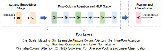
Figure 15.
Flowchart of the neural network for data security risk assessment.
For a dataset containing N data samples, each sample has features, and denotes the number of risk levels.
1. Input and embedding
(1) Input Data
Let represent the raw scalar input, where denotes the i-th sample and denotes the f-th feature value of the corresponding sample. All samples are arranged into a matrix , where the element in the i-th row and f-th column of is .
(2) Scalar Mapping
Define a set of learnable parameters and , where D denotes the embedding dimension of the network. Each scalar is mapped to a D-dimensional space:
where and corresponds to the full vector in the embedding space for the f-th feature of the i-th sample.
(3) Learnable Vector of Feature Columns
For each feature column f, let denotes its learnable identifier vector. There are F such vectors, denoted
These vectors are added to the f-th column of , with each element computed as
where is the embedding tensor before entering the row–column attention layer.
2. Multilayer row–column attention and MLP
Assume that the network stacks L layers, with each layer’s input and output in . Let
for , where is the embedding input obtained from the previous step. The specific structure of each layer includes three components, detailed as follows.
(1) Intra-Row Attention: Let . Define trainable matrices (for multi-head attention, D is partitioned into and processed in parallel). Denote
Then, compute
Apply residual connections and layer normalization to obtain the intra-row attention result .
(2) Intra-Column Attention: Let . Define another set of trainable matrices , , and . Denote
Then, compute the following formula.
Apply residual connections and layer normalization to obtain the intra-column attention result .
In the row–column attention mechanism, the input is essentially mapped to Query–Key–Value. However, intra-row attention treats “different features of the same sample” as a sequence. By iteratively computing along these two dimensions, the model can simultaneously represent dependencies among features and samples.
(3) MLP Sub-layer: The MLP sub-layer includes two fully connected layers. Let
Define
Then, apply besidual connections and layer normalization to to obtain the output of the layer . So far, we have finished the computation for one layer.
3. Pooling and classification
After multiple iterations, the output is obtained. For each sample i, average pooling is performed along the feature dimension F:
After aggregating all samples, the pooled result is given by . Then, define the linear layer weights and bias and compute the final multi-class as
Then, employ a conventional cross-entropy loss function to perform data risk level prediction classification. The cross-entropy loss fuction is formulated as
where denotes the actual risk level label of the i-th sample, and represents the unnormalized output score of the i-th sample for class c. Meanwhile, denotes the output score of the i-th sample under its label .
5. Experimental Verification and Comparative Analysis
Based on our proposed data risk assessment method, we conduct a safety risk assessment for the full lifecycle security of gas data inside a gas system. Our experimental environment is shown in Table 9.
Table 9.
Experimental environment configuration.
5.1. Dataset Collection and Preprocessing
The data collection process was conducted in accordance with the specific requirements of the evaluation metrics defined for each phase of the data’s full lifecycle under the proposed scheme. A hybrid approach combining automated and manual data collection methods was adopted. For the collected data, relevant features were extracted to retain the information most pertinent to the evaluation metrics. Subsequently, metric quantification was performed based on the internal security requirements of the gas system and the quantification rules specified in our scheme. To ensure the accuracy of the experimental results, we excluded the samples whose index missing rate reached 10%. As a result, a total of 5761 valid data samples were obtained, with each sample comprising 30 quantified metric values.
Some contents are shown in Table 10.
Table 10.
Preprocessed dataset.
5.2. Determination of Indicator Weights
According to this scheme, the indicator weights are mainly derived from two dimensions: the subjective weights are obtained through AHP, and the objective weights are calculated using EWM. Finally, we obtain the specific indicator weights for the risk assessment of the gas system by weighting these two components.
5.2.1. Subjective Weight Determination Using the AHP
When using the Analytic Hierarchy Process to determine the subjective weights of the risk assessment indicators for the gas system’s entire data lifecycle, the process involves constructing the judgment matrix, calculating the weight vector, performing consistency checks, and other procedures. Based on this, the final subjective indicator weights for the data lifecycle are calculated for the dataset.
1. Construction of the judgment matrix of each stage
This scheme collects the indicator judgment matrices from 12 experts in the field of data security risk. By integrating these experts’ judgment matrices using the geometric mean method, we obtain the final judgment matrix, shown as follows:
(1) Table 11 presents the pairwise comparison matrix of security risk assessment indicators in the data collection phase.
Table 11.
Data collection security risk assessment indicator judgment matrix.
(2) Table 12 presents the pairwise comparison matrix of security risk assessment indicators in the data transmission phase.
Table 12.
Data transmission security risk assessment indicator judgment matrix.
(3) Table 13 presents the pairwise comparison matrix of security risk assessment indicators in the data storage phase.
Table 13.
Data storage security risk assessment indicator judgment matrix.
(4) Table 14 presents the pairwise comparison matrix of security risk assessment indicators in the data processing phase.
Table 14.
Data processing security risk assessment indicator judgment matrix.
(5) Table 15 presents the pairwise comparison matrix of security risk assessment indicators in the data exchange phase.
Table 15.
Data exchange security risk assessment indicator judgment matrix.
(6) Table 16 presents the pairwise comparison matrix of security risk assessment indicators in the data destruction phase.
Table 16.
Data destruction security risk assessment indicator judgment matrix.
2. Calculation of the weight vector of each stage
By calculation, we obtain the weight vector for the lifecycle indicators for the gas system data security risk assessment, shown as follows.
The weight vectors for each lifecycle indicator for the gas system data security risk assessment are calculated as follows.
(1) The weight vector for the data collection stage is
(2) The weight vector for the data transmission stage is
(3) The weight vector for the data storage stage is
(4) The weight vector for the data processing stage is
(5) The weight vector for the data exchange stage is:
(6) The weight vector for the data destruction stage is
3. Consistency check
The consistency index of the judgment matrix for each lifecycle stage is computed as follows.
(1) Data collection stage:
(2) Data transmission stage:
(3) Data storage stage:
(4) Data processing stage:
(5) Data exchange stage:
(6) Data destruction stage:
Since the values for all stages satisfy , all judgment matrices have been verified to satisfy the established consistency requirements, and the indicator weights for each stage meet the requirements.
4. Determination of the final subjective indicator weights
In this experiment, based on data characteristics and the requirements of application scenario, the experts assign the weights of each period as follows:
Then, according to the condition , we obtain the final subjective indicator weights for the entire data lifecycle, shown as follows.
(1) Table 17 shows the subjective weights for each indicator in the data collection stage.
Table 17.
Subjective indicator weights for the data collection stage.
(2) Table 18 shows the subjective weights for each indicator in the data transmission stage.
Table 18.
Subjective indicator weights for the data transmission stage.
(3) Table 19 shows the subjective weights for each indicator in the data storage stage.
Table 19.
Subjective indicator weights for the data storage stage.
(4) Table 20 shows the subjective weights for each indicator in the data processing stage.
Table 20.
Subjective indicator weights for the data processing stage.
(5) Table 21 shows the subjective weights for each indicator in the data exchange stage.
Table 21.
Subjective indicator weights for the data exchange stage.
(6) Table 22 shows the subjective weights for each indicator in the data destruction stage.
Table 22.
Subjective indicator weights for the data destruction stage.
It can be verified that the sum of all indicator weights is 1.
5.2.2. Objective Weight Determination Using EWM
When using the Entropy Weight Method to calculate the objective weights of the risk assessment indicators for the gas system’s entire data lifecycle, the process involves data normalization, calculation of the probability matrix, calculation of information entropy, and calculation of entropy weights. Based on this process, the final objective indicator weights for the data lifecycle are calculated for the dataset as follows.
(1) Table 23 presents the objective weights for each indicator in the data collection stage.
Table 23.
Objective weights for the indicators in the data collection stage.
(2) Table 24 presents the objective weights for each indicator in the data transmission stage.
Table 24.
Objective weights for the indicators in the data transmission stage.
(3) Table 25 presents the objective weights for each indicator in the data storage stage.
Table 25.
Objective weights for the indicators in the data storage stage.
(4) Table 26 presents the objective weights for each indicator in the data processing stage.
Table 26.
Objective weights for the indicators in the data processing stage.
(5) Table 27 presents the objective weights for each indicator in the data exchange stage.
Table 27.
Objective weights for the indicators in the data exchange stage.
(6) Table 28 presents the objective weights for each indicator in the data destruction stage.
Table 28.
Objective weights for the indicators in the data destruction stage.
It can be verified that the sum of all indicator weights is 1.
5.2.3. Comprehensive Weight Determination
The composite weight is determined by the following formula:
In this experiment, the balancing coefficient is chosen as , i.e.,
By aggregating the indicator weights determined by AHP and EWM, we obtain the final composite indicator weights for the entire data lifecycle, shown as follows.
(1) Table 29 presents the comprehensive weights for each indicator in the data collection stage.
Table 29.
Comprehensive weights for the indicators in the data collection stage.
(2) Table 30 presents the comprehensive weights for each indicator in the data transmission stage.
Table 30.
Comprehensive weights for the indicators in the data transmission stage.
(3) Table 31 presents the comprehensive weights for each indicator in the data storage stage.
Table 31.
Comprehensive weights for the indicators in the data storage stage.
(4) Table 32 presents the comprehensive weights for each indicator in the data processing stage.
Table 32.
Comprehensive weights for the indicators in the data processing stage.
(5) Table 33 presents the comprehensive weights for each indicator in the data exchange stage.
Table 33.
Comprehensive weights for the indicators in the data exchange stage.
(6) Table 34 presents the comprehensive weights for each indicator in the data destruction stage.
Table 34.
Comprehensive weights for the indicators in the data destruction stage.
It can be verified that the sum of all indicator weights is 1. The chart depicting the indicator weight proportions is shown in Figure 16.
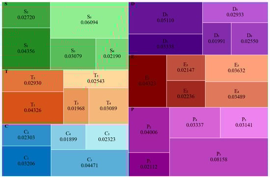
Figure 16.
Distribution chart of indicator weights in full lifecycle gas system data risk evaluation.
From the proportion chart of indicator weights, it is clear that the weights of different indicators in the full lifecycle safety risk assessment of the gas system vary significantly. Based on this chart, security personnel can allocate resources more effectively by focusing on the most critical areas, thereby enhancing relevant protective capabilities in a targeted manner. For example, integrating both subjective and objective perspectives, the data and chart reveal that indicator has the highest weight, with a proportion of 8.158%, indicating it has the greatest impact on the overall assessment results. This finding suggests that in order to achieve refined data security protection within this gas system, special attention should be paid to issues related to data leakage.
5.3. Risk Level Labeling
For each data sample in the dataset, we use the fuzzy comprehensive evaluation method to label the risk level.
1. Determination of the evaluation indicator set
When labeling risk levels for the quantified data samples, we adopt the the entire data lifecycle risk assessment indicator system U proposed in this scheme as the evaluation indicator set, which is defined as follows.
2. Determination of the evaluation level set
In the experiment, we set the evaluation level according to the proposed scheme, shown as follows:
3. Determination of the evaluation indicator weights
The weights for each indicator are those determined comprehensively by the AHP-EMW based method in Section 5.2, namely,
4. Construction of the fuzzy evaluation matrix
For a given data sample, the fuzzy evaluation matrix is built using its quantified indicator values. Taking the following data sample as an example, we have
Using the above sample, the steps for constructing the fuzzy evaluation matrix are described as follows.
(1) For the value corresponding to indicator , since , the membership degree for high risk is 1, and the membership degrees for the other risk levels are 0. Therefore, the membership vector is .
(2) Following the approach in step (1), the membership vectors are sequentially calculated for the remaining indicator values.
(3) Using the results from step (2), the fuzzy evaluation matrix is constructed by taking the vectors to as its rows, yielding .
5. Fuzzy comprehensive evaluation
The fuzzy comprehensive evaluation formula is given as follows:
By applying the aforementioned formula, the fuzzy comprehensive evaluation vector for this data sample is computed as follows:
Since the membership degree for high risk is the highest, this data sample is labeled high risk, denoted 3 in the dataset.
The labeled part of the dataset is shown in Table 35.
Table 35.
Labeled dataset.
5.4. Training the Neural Network Model
In this study, we train the neural network model using the parameter settings defined in Table 36.
Table 36.
Parameter settings for neural network training.
The experimental results of training the neural network model for risk assessment are shown in Table 37.
Table 37.
Experimental results.
In the experiment, among the 1153 test samples in the test set, 97.14% of the samples were correctly classified, and the macro-precision reached 97.13%, indicating that the model has high prediction accuracy in each risk level (low, medium, and high). Similarly, after calculating the recall rate for each category, the macro-recall rate is 97.25%, indicating that the model has excellent ability to identify all types of samples. The macro F1-score considers both accuracy and recall, and its value of 97.15% indicates that the model performs very well in balancing these two as well.
By subdividing the experimental results into specific risks, the confusion matrix of experimental results is as follows:
According to the confusion matrix, there are a total of 376 actual low-risk samples, of which 369 were exactly classified as low risk, 6 were misclassified as medium risk, and 1 was incorrectly labeled as high risk. There are 364 actual medium-risk samples, of which 360 were accurately classified as medium risk, 4 were incorrectly labeled as low risk, and none were misclassified as high risk. There are 413 actual high-risk samples, of which 391 were rightly classified as high risk, 2 were incorrectly labeled as low risk, and 20 were mislabeled as medium risk. The confusion matrix indicates that the predictions for the low-risk and medium-risk categories are relatively accurate, with very few misclassifications; however, 20 high-risk samples were erroneously predicted as medium risk, suggesting that there is still some ambiguity at the boundary between high risk and medium risk. Nonetheless, the overall accuracy remains very high.
The experimental results indicate that the model achieved high accuracy, precision, recall, and F1-scores across all categories, demonstrating that its ability to identify each risk level is well balanced and that it exhibits strong generalization performance and robustness in the risk assessment task. In the data security risk assessment task, the high accuracy and balanced performance across categories suggest that the model can reliably determine risks across the entire data lifecycle, thereby providing robust support for practical risk management and decision making.
5.5. Comparative Analysis
5.5.1. Comparison with Related Schemes
This section mainly compares the data security risk assessment scheme proposed in this paper with other representative data security risk assessment schemes of recent years. The comparative results are presented in Table 38.
Table 38.
Comparison of different risk assessment schemes.
From the above table, it can be seen that the proposed data security risk assessment scheme exhibits outstanding performance in application domain adaptability and multidimensional coverage of index system. By constructing an attention-based neural network architecture and performing supervised learning with a labeled dataset obtained using the fuzzy comprehensive evaluation method, the proposed approach markedly improves both generalization and predictive accuracy, thereby effectively meeting risk assessment requirements in complex scenarios. Compared to traditional static assessment paradigms, this scheme achieves automated feature engineering and self-adaptive optimization of model parameters while innovatively refining the evaluation granularity to the full lifecycle dimension of data assets, thereby providing an interpretable technical pathway for precise risk quantification.
5.5.2. Model Performance Comparison
Based on an analysis of current research articles in the risk assessment field, the domain primarily employs two algorithms, namely Artificial Neural Networks (ANNs) and Support Vector Machines (SVMs) [40]. Table 39 shows their characteristics.
Table 39.
Comparison of ANN and SVM.
Performance comparisons were conducted among the proposed scheme, the Support Vector Machine, and a classical feedforward neural network (FFNN). The experimental dataset was used as input, and the results are shown in Table 40.
Table 40.
Training results of the SVM model and the FFNN model.
In this comparative experiment, after global parameter optimization, the SVM model achieved approximately overall accuracy on the data security risk assessment task, with other metrics—macro-precision, macro-recall, and macro-F1 score—also around . In contrast, the FFNN model’s performance was suboptimal, with all evaluation metrics around , primarily because ANN models require larger datasets and perform poorly on small-scale datasets.
The confusion matrix of the SVM model’s experimental results is as follows:
The confusion matrix of the FFNN model’s experimental results is as follows:
The confusion matrix indicates that both models—especially the FFNN—perform poorly in small-sample risk assessment environments. In practical data security risk assessment scenarios, misclassifying data of different levels may lead to different types of serious consequences.
(1) If low-risk data are misclassified as medium or high risk, it may lead to excessive allocation of security management resources and budget.
(2) If medium-risk data are misclassified as low risk, it may reduce vigilance toward medium-risk events, thereby delaying the identification and response to potential threats and increasing the likelihood of security incidents. Conversely, misclassifying medium-risk data as high risk causes events of moderate risk to receive excessive attention, which may lead to resource wastage and trigger unnecessary security measures and emergency responses, thereby disrupting normal business operations.
(3) If high-risk data are misclassified as low or medium risk, it results in the most severe consequences, because it implies that genuinely high-risk security incidents have not been identified in a timely manner. This underestimation of risk may lead to the neglect of critical vulnerabilities and threats, resulting in insufficient security measures and potentially exposing the given enterprise to major security incidents or data breaches.
From the confusion matrix results, it can be observed that both models exhibit some misclassification across different risk levels. A detailed comparison with the model used in this scheme is shown in Figure 17.
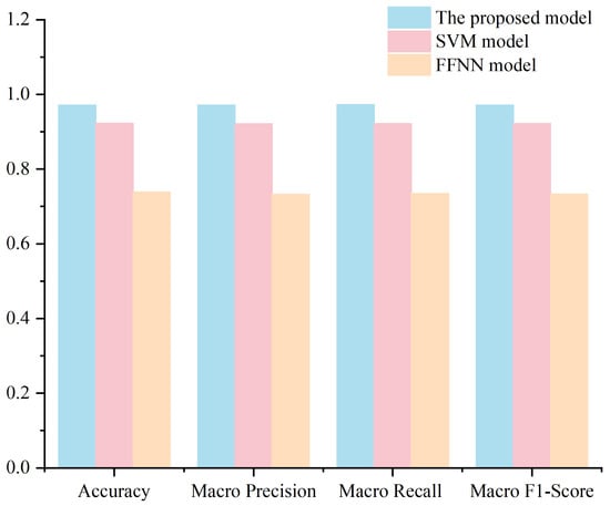
Figure 17.
Performance comparison of our scheme with the SVM model and the FFNN model.
As illustrated in the above figure, the model proposed in this paper outperforms the other two schemes across every evaluation metric, while the FFNN model exhibits the weakest performance. These results attest to the efficacy and robustness of our approach for data security risk assessment; it effectively exploits inter-feature relationships, high-order interactions, and inter-sample information, thereby delivering a stronger representational capacity than purely kernel-based methods or shallow neural networks.
In small-sample data security risk assessment scenarios, the proposed model offers the following advantages:
(1) Automatic capture of high-order feature interactions: The proposed model employs intra-row attention to model interactions among the 30 quantified indicators within each sample, thereby automatically learning the complex relationships between indicators; simultaneously, it utilizes intra-column attention to integrate information for the same indicator across different samples, extracting global feature patterns and automatically capturing these high-order interactions during training.
(2) Nonlinear representation and end-to-end training: The proposed model incorporates a multilayer perceptron sub-layer, where each layer applies a nonlinear activation function to more effectively capture complex relationships in the input data. In contrast, other models often require extensive parameter tuning in practical applications and may need to be re-tuned for different datasets; they also incur high computational costs on high-dimensional data and impose certain requirements on training dataset size.
Therefore, based on a row–column bidirectional attention mechanism, our proposed data security risk assessment model automatically captures high-order nonlinear feature interactions both within and across samples. By leveraging end-to-end training, it achieves greater accuracy, flexibility, and efficiency in real-world risk assessment tasks and demonstrates a clear advantage over the methods typically employed in full lifecycle data security risk evaluation.
5.6. Sensitivity Analysis
In real-world environments, data collection for data security risk assessment may be affected by measurement errors, noise injection, and network jitter. Since different data security risk assessment indicators correspond to distinct types of security risks, to verify the robustness of this scheme under different disturbance scenarios, we conducted sensitivity analysis experiments under different noises separately and quantified the sensitivity of the model performance varying with the disturbance amplitude at the same time.
(1) Experimental Design
In the experiment, Gaussian noise with a relative amplitude of was injected into each dimension of the test set samples :
where , . is regarded as the baseline. This design makes the noise variance proportional to the characteristic amplitude.
(2) Evaluation Metrics
For each perturbation level, inference was repeated three times, and four evaluation metrics were computed: accuracy, macro-precision, macro-recall, and macro-F1-score.
The experimental results under different Gaussian noise levels are summarized in Table 41.
Table 41.
Experimental eesults under different Gaussian noise levels.
According to the experimental results, the performance of the proposed model remains nearly unchanged under continuous noise perturbations, demonstrating strong tolerance to common measurement errors. This ensures the stability and reliability of risk assessment across the entire data lifecycle. The results of the sensitivity analysis confirm that the model exhibits significant robustness within the range of common errors, providing experimental support for its reliable deployment in practical data security risk assessment scenarios.
6. Conclusions
This study focuses on the security risk assessment of the full data lifecycle, and its main contributions are as follows.
(1) Constructing a security risk assessment indicator system for the full data lifecycle: This study proposes a general security risk assessment indicator system that systematically covers the entire lifecycle of data, from collection to destruction, ensuring the completeness and systematicity of risk assessment dimensions.
(2) Allocating multidimensional weights to evaluation indicators: To ensure the scientific rigor and fairness of indicator weighting, this study adopts a combination of the Analytic Hierarchy Process and the Entropy Weight Method to allocate indicator weights from both subjective and objective perspectives. This approach effectively improves the comprehensiveness and accuracy of weight assignment, thereby enhancing the credibility of the risk assessment results.
(3) Proposing an attention-based neural network model for data security risk assessment: For the collected training dataset, this study first applies the fuzzy comprehensive evaluation method to perform scientific and reasonable fine-grained risk level annotation. Subsequently, a neural network model integrating attention mechanism across both row and column dimensions is constructed and trained. This model can make full use of the dual information interaction of the risk assessment dataset in the indicator dimension and the sample dimension. Experimental results demonstrate that, after training on a moderate-sized dataset, the model exhibits high accuracy and strong generalization ability in risk assessment tasks on new data. Compared with traditional methods, this model significantly improves the precision and granularity of the risk assessment results by automatically learning complex patterns and nonlinear relationships in the sample data, thereby reducing bias introduced by human factors. In addition, the model continuously performs iterative optimization, adaptively updating its parameters to respond to data changes, maintaining high flexibility and usability in practical applications, and adapting to evolving risk environments.
This scheme can be used not only for overall security risk assessment across the entire data lifecycle but also for phase-specific assessments of each lifecycle stage. It enables dynamic monitoring of data security conditions at different periods, helping decision makers to comprehensively understand the risk levels of each stage and providing a solid foundation for formulating precise and effective security management strategies. Moreover, since risk assessment results directly influence resource allocation, reinforcement planning, and emergency response strategies, extremely high accuracy is required in the risk assessment process. Therefore, compared with traditional methods, this scheme is particularly suitable for real-world scenarios in which data acquisition is costly or sample sizes are limited. In small-sample environments, it demonstrates a significant advantage in data security risk assessment.
Future research will further advance in the following directions.
(1) Development of a more refined data security risk assessment indicator system: The current study designs 30 indicators for data full lifecycle risk assessment. Future research should further refine the security risk factors associated with each lifecycle phase and design a more targeted quantitative risk assessment indicator system. This will not only improve the precision of risk identification and measurement but also provide robust theoretical support and practical guidance for risk management practices.
(2) Further improvement of model performance: Although the current model already achieves a high level of accuracy, to enhance its expressiveness in capturing nonlinear relationships and complex risk patterns, future research may explore the integration of new models such as graph neural networks to optimize current model performance, further improving the accuracy of data security risk prediction and the model’s generalization capabilities.
(3) Further research on data security early warning and incident response: Building upon this study, future work will focus on two key areas—data security early warning and data security incident response. The goal is to significantly enhance the depth of proactive defense against complex data security threats and the efficiency of emergency responses, thereby providing a more solid and reliable security guarantee for digital business environments.
Author Contributions
Conceptualization, J.L. and T.H.; methodology, T.H.; software, J.Z.; validation, J.L., T.H. and J.Z.; formal analysis, T.H. and D.M.; investigation, J.Z. and D.M.; data curation, H.L.; writing—original draft preparation, T.H. and H.L.; writing—review and editing, J.Z. and B.T.; supervision, B.T. and J.L. All authors have read and agreed to the published version of the manuscript.
Funding
This work was supported by the Shenzhen Science and Technology Innovation and Entrepreneurship Plan (KJZD20230923114906013), the National Natural Science Foundation of China (62272389), and the Shenzhen Basic Research Program (20210317191843003).
Data Availability Statement
The dataset used in this study is confidential and therefore cannot be made publicly available. However, this paper provides a detailed description of the dataset annotation, training process, and related procedures, which readers can refer to for further understanding.
Conflicts of Interest
The authors declare no conflicts of interest.
References
- Chen, X.; He, Y.; Pakdel, G.H.; Liu, X.; Wang, S. A comprehensive multi-stage decision-making model for supplier selection and order allocation approach in the digital economy. Adv. Eng. Inform. 2025, 63, 102961. [Google Scholar] [CrossRef]
- Chen, Z.; Zhang, Z.; Yang, Z. Big AI models for 6G wireless networks: Opportunities, challenges, and research directions. IEEE Wirel. Commun. 2024, 31, 164–172. [Google Scholar] [CrossRef]
- Samaraweera, G.D.; Chang, J.M. Security and privacy implications on database systems in big data era: A survey. IEEE Trans. Knowl. Data Eng. 2019, 33, 239–258. [Google Scholar] [CrossRef]
- Jeong, D.; Kim, J.H.T.; Im, J. A new global measure to simultaneously evaluate data utility and privacy risk. IEEE Trans. Inf. Forensics Secur. 2022, 18, 715–729. [Google Scholar] [CrossRef]
- Kuang, X.; Hong, C.; Jiang, Y.; Zhang, Y.; Yang, Y.; Li, P. Research on the new generation of network data security protection technology for zero-trust environment. In Proceedings of the 2024 IEEE 4th International Conference on Data Science and Computer Application, Dalian, China, 22–24 November 2024; pp. 337–341. [Google Scholar]
- Siami, M.; Naderpour, M.; Ramezani, F.; Lu, J. Risk assessment through big data: An autonomous fuzzy decision support system. IEEE Trans. Intell. Transp. Syst. 2024, 25, 9016–9027. [Google Scholar] [CrossRef]
- Bethlehem, J.G.; Keller, W.J.; Pannekoek, J. Disclosure control of microdata. J. Am. Stat. Assoc. 1990, 85, 38–45. [Google Scholar] [CrossRef]
- Wairimu, S.; Iwaya, L.H.; Fritsch, L.; Lindskog, S. On the evaluation of privacy impact assessment and privacy risk assessment methodologies: A systematic literature review. IEEE Access. 2024, 12, 19625–19650. [Google Scholar] [CrossRef]
- Hariharan, A. Cluster-based risk analysis for big data security framework. In Proceedings of the 2024 7th International Conference on Circuit Power and Computing Technologies, Kollam, India, 8–9 August 2024; pp. 1085–1090. [Google Scholar]
- Zhan, H.; Yang, J.; Guo, Z.; Cao, J.; Zhang, D.; Zhao, X.; You, W.; Li, H. RiskTree: Decision trees for asset and process risk assessment quantification in big data platforms. Secur. Saf. 2024, 3, 2024009. [Google Scholar] [CrossRef]
- Munodawafa, F.; Awad, A.I. Security risk assessment within hybrid data centers: A case study of delay sensitive applications. J. Inf. Secur. Appl. 2018, 43, 61–72. [Google Scholar] [CrossRef]
- Wang, L.; Jin, L.; Ji, H.; Wang, J.; Chen, Y.; Fang, J. Data Security Risk Assessment Method of Intelligent and Connected Vehicles Based on Data Security Classification and Grading. In Proceedings of the 2023 IEEE 8th International Conference on Intelligent Transportation Engineering, Beijing, China, 28–30 October 2023; pp. 165–171. [Google Scholar]
- Liu, D.; Liu, Z.; Liu, Y.; Qiu, B.; Wang, S. Research on automobile data security risk analysis based on TARA method. In Proceedings of the 2024 IEEE 9th International Conference on Data Science in Cyberspace, Jinan, China, 23–26 August 2024; pp. 162–170. [Google Scholar]
- Zhou, S.; Yang, X.; Li, M.; Yang, H.; Ji, H. Data Security Risk Assessment Method for Connected and Automated Vehicles. In Proceedings of the 2022 IEEE 7th International Conference on Intelligent Transportation Engineering, Beijing, China, 11–13 November 2022; pp. 379–387. [Google Scholar]
- Ba, Z.; Wang, Y.; Fu, J.; Li, Y.; Liu, X. Corrosion Risk Assessment Model of Gas Pipeline Based on Improved AHP and Its Engineering Application. Arab. J. Sci. Eng. 2022, 47, 10961–10979. [Google Scholar] [CrossRef]
- Melgarejo, D.N.; Flentge, F.; Eggleston, J. Security Risk Assessment and Management for ESOC’s Mission Operations Infrastructure Data Systems. In Proceedings of the 2014 Conference on SpaceOps, Pasadena, CA, USA, 5–9 May 2014. [Google Scholar]
- Alvim, M.S.; Fernandes, N.; McIver, A.; Morgan, C.; Nunes, G.H. Flexible and scalable privacy assessment for very large datasets, with an application to official governmental microdata. In Proceedings of the 2022 International Conference on Privacy Enhancing Technologies, Washington, DC, USA, 31 August 2022. [Google Scholar]
- Alonge, C.Y.; Arogundade, O.T.; Adesemowo, K.; Ibrahalu, F.T.; Adeniran, O.J.; Mustapha, A.M. Information asset classification and labelling model using fuzzy approach for effective security risk assessment. In Proceedings of the 2020 International Conference in Mathematics, Computer Engineering and Computer Science, Lagos, Nigeria, 18–21 March 2020; pp. 1–7. [Google Scholar]
- Hussaini, S.S.; Raharjo, B. Comprehensive Risk Evaluation Model for Data Center Security Risk Assessment. In Proceedings of the 2024 10th International Conference on Wireless and Telematics, Batam, Indonesia, 4–5 July 2024; pp. 1–6. [Google Scholar]
- Hossain, N.; Das, T.; Islam, T.; Alam Hossain, M. Cyber security risk assessment method for SCADA system. Inf. Secur. J. Glob. Perspect. 2022, 31, 499–510. [Google Scholar] [CrossRef]
- Bitton, R.; Maman, N.; Singh, I.; Momiyama, S.; Elovici, Y.; Shabtai, S. Evaluating the Cybersecurity Risk of Real-world, Machine Learning Production Systems. ACM Comput. Surv. 2023, 55, 1–36. [Google Scholar] [CrossRef]
- Zhang, X.; Guo, T. Privacy Risk Assessment of Medical Big Data Based on Information Entropy and FCM Algorithm. IEEE Access 2024, 12, 148190–148200. [Google Scholar] [CrossRef]
- Bai, Y.; Wu, J.; Ren, Q.; Jiang, Y.; Cai, J. A BN-Based Risk Assessment Model of Natural Gas Pipelines Integrating Knowledge Graph and DEMATEL. Process Saf. Environ. Prot. 2023, 171, 640–654. [Google Scholar] [CrossRef]
- Zhang, X.; Shen, W.; Liang, Z.; Cui, L.; Wang, Y. Data Security Risk Assessment Method Based on Big Data Technology. In Proceedings of the 2024 IEEE 16th International Conference on Computational Intelligence and Communication Networks, Indore, India, 22–23 December 2024; pp. 589–594. [Google Scholar]
- Meng, C.; Meng, L.; Chen, L.; Liao, D. Research on Neural Network Algorithm in Risk Assessment of Network Security Spatial Data Assets. In Proceedings of the 2024 5th International Conference on Artificial Intelligence and Electromechanical Automation, Shenzhen, China, 14–16 June 2024; pp. 245–250. [Google Scholar]
- Huang, B.; Wei, J.; Tang, Y.; Chang, L. Enterprise risk assessment based on machine learning. Comput. Intell. Neurosci. 2021, 1, 6049195. [Google Scholar] [CrossRef]
- Muhammad, A.H.; Nasiri, A.; Harimurti, A. Machine learning methods for classification and prediction information security risk assessment. IAES Int. J. Artif. Intell. 2025, 14, 457–465. [Google Scholar] [CrossRef]
- Brauwers, G.; Frasincar, F. A general survey on attention mechanisms in deep learning. IEEE Trans. Knowl. Data Eng. 2021, 35, 3279–3298. [Google Scholar] [CrossRef]
- Yong, S.; Junyu, Y.; Miaoyan, T.; Jiatao, D.; Hao, J. Situation assessment model based on attention mechanism data fusion for the new-type power system. In Proceedings of the 2024 IEEE 7th International Conference on Information Systems and Computer Aided Education, Dalian, China, 27–29 September 2024; pp. 113–119. [Google Scholar]
- Liu, Y.; Sun, Y.; Liu, C.; Weng, Y. Industrial Internet security situation assessment method based on self-attention mechanism. In Proceedings of the 2024 3rd International Conference on Artificial Intelligence, Internet of Things and Cloud Computing Technology, Wuhan, China, 13–15 September 2024; pp. 148–151. [Google Scholar]
- Chen, J.; Bian, H.; Liang, H. A network security situation prediction model enhanced by multi-head attention mechanism. Informatica 2025, 49, 18. [Google Scholar] [CrossRef]
- Xiao, X.; Chen, H.; Zhang, Y.; Ren, W.; Xu, J.; Zhang, J. Anomalous payment behavior detection and risk prediction for SMEs based on LSTM-attention mechanism. Acad. J. Sociol. Manag. 2025, 3, 43–51. [Google Scholar] [CrossRef]
- Chen, C.; Quan, W.; Shao, Z. Aerial target threat assessment based on gated recurrent unit and self-attention mechanism. J. Syst. Eng. Electron. 2024, 35, 361–373. [Google Scholar] [CrossRef]
- Rezapour, M.; Yazdinejad, M.; Rajabi Kouchi, F.; Baghi, M.H.; Khorrami, Z.; Zadeh, M.K.; Pourbaghi, E.; Rezapour, H. Text mining of hypertension researches in the West Asia region: A 12-year trend analysis. Renal Failure 2024, 46, 2337285. [Google Scholar] [CrossRef] [PubMed]
- Samizadeh, R.; Zadeh, M.K.; Jadidi, M.; Rezapour, M.; Vatankhah, S. Discovery of dangerous self-medication methods with patients, by using social network mining. Int. J. Bus. Intell. Data Min. 2023, 23, 277–287. [Google Scholar] [CrossRef]
- Rezapour, M.; Asadi, R.; Marghoob, B. Machine learning algorithms as new screening framework for recommendation of appropriate vascular access and stroke reduction. Int. J. Hosp. Res. 2021, 10. [Google Scholar]
- Zhang, B.; Pedrycz, W.; Fayek, A.R.; Dong, Y. A differential evolution-based consistency improvement method in AHP with an optimal allocation of information granularity. IEEE Trans. Cybern. 2020, 52, 6733–6744. [Google Scholar] [CrossRef] [PubMed]
- Qin, T.; Liu, M.; Ji, S.; Cai, D. Parameter Weight Analysis of Synchronous Induction Electromagnetic Coil Launch System Based on the Entropy Weight Method. IEEE Trans. Plasma Sci. 2024, 52, 1865–1873. [Google Scholar] [CrossRef]
- Hollmann, N.; Müller, S.; Purucker, L.; Krishnakumar, A.; Körfer, M.; Hoo, H.B.; Schirrmeister, R.T.; Hutter, F. Accurate predictions on small data with a tabular foundation model. Nature 2025, 637, 319–326. [Google Scholar] [CrossRef]
- Hegde, J.; Rokseth, B. Applications of machine learning methods for engineering risk assessment–A review. Saf. Sci. 2020, 122, 104492. [Google Scholar] [CrossRef]
Disclaimer/Publisher’s Note: The statements, opinions and data contained in all publications are solely those of the individual author(s) and contributor(s) and not of MDPI and/or the editor(s). MDPI and/or the editor(s) disclaim responsibility for any injury to people or property resulting from any ideas, methods, instructions or products referred to in the content. |
© 2025 by the authors. Licensee MDPI, Basel, Switzerland. This article is an open access article distributed under the terms and conditions of the Creative Commons Attribution (CC BY) license (https://creativecommons.org/licenses/by/4.0/).