C¹ Shape-Preserving Rational Quadratic/Linear Interpolation Splines with Necessary and Sufficient Conditions

Abstract

In this work, we introduce a novel class of $C^1$ rational quadratic interpolation splines defined by two symmetric parameters. This generalization encompasses the rational quadratic interpolation schemes given by Schmidt in 1987 as a special case. For data sets with convexity, monotonicity, or positivity constraints, we derive the necessary and sufficient conditions, ensuring that the interpolant preserves these properties. Furthermore, we propose an algorithm for selecting visually appealing and shape-preserving spline curves by minimizing a particular approximated curvature functional.

1. Introduction

With the development of computer graphics (CG), computer-aided design (CAD), computer aided geometric design (CAGD), and scientific data visualization in engineering, constructing visually pleasing shape-preserving interpolation spline curves for positive, monotone, and/or convex sets of data being interpolated is an essential problem and has attracted widespread interest. In the past, various shape-preserving interpolation spline methods have been proposed; among the multitude of references on this subject, the reader is referred to the comprehensive reviews by Kvasov [1] and Goodman [2], where systematic comparisons and analyses of existing algorithms for shape-preserving spline interpolation are provided.

Piecewise rational quadratic and cubic spline methodologies have been extensively researched for developing shape-preserving interpolation splines. Multiple specialized rational cubic interpolation splines have been formulated for the graphical representation of strictly positive data sets by Hussain and Sarfraz [3], Sarfaze [4], and Qin et al. [5]. Some specific rational cubic monotonicity-preserving interpolants have been proposed by Gregory [6], Sarfraz [7,8], Hussain and Hussain [9], Sarfraz et al. [10], and Abbas et al. [11]. Various rational cubic splines have been constructed by Delbourgo [12], Sarfraz and Hussain [13], Sarfraz et al. [14], and Abbas et al. [15] to produce convexity-preserving interpolation curves for convex data sets. These shape-preserving rational cubic interpolants typically achieve $C^1$ continuity, whereas $C^2$ continuity requires solving linear/nonlinear systems of compatibility equations for derivative specifications at knots; see the corresponding methods described in Delbourgo [12] and Abbas et al. [15]. Recently, by using weighted $C^1$ quadratic and cubic splines, Kvasov developed weighted $C^1$ quadratic/cubic spline algorithms with automated weight selection mechanisms for generating shape-preserving interpolants specific to monotonic or convex data sets; see Kvasov [16,17,18]. Some $C^2$ rational quartic shape-preserving interpolation splines were designed by Han [19,20], Zhu and Han [21], and Zhu [22,23], avoiding solving global linear/nonlinear compatibility equation systems. However, the shape-preserving conditions of these methods are just sufficient but not necessary.

When constructing shape-preserving interpolation splines, a necessary and sufficient condition can always bring much convenience. For example, it can precisely judge whether the splines preserve the shape or not and estimate practicability. Therefore, the key aim of this paper is to find the necessary and sufficient conditions. There are a few papers concerning the construction of $C^1$ shape-preserving interpolation splines with sufficient and necessary conditions. In [24], Schmidt developed a kind of $C^1$ rational quadratic interpolation splines with a parameter, with a necessary and sufficient criterion to ensure the property of positivity carries over from the data set. The criterion can always be satisfied if the parameters are properly chosen. Later, in [25], Schmidt constructed a class of $C^1$ quadratic and related exponential interpolation splines and discussed and deduced sufficient and necessary conditions for the interpolant preserving monotonicity and/or convexity.

In this work, we construct a kind of $C^1$ rational quadratic interpolation spline possessing two symmetric parameters, which include the positivity-preserving rational quadratic interpolation splines with a parameter given in [24] as a special case. Furthermore, the necessary and sufficient conditions for the new rational quadratic interpolation splines preserving convexity, monotonicity, and positivity are also developed. The rest of this paper is organized as follows. Section 2 gives the construction of the new $C^1$ rational quadratic interpolation spline with two symmetric parameters. Furthermore, the necessary and sufficient conditions of the proposed interpolation spline to preserve the shape of convex, monotonic, and positive sets of data are derived. In Section 3, a particular approximated curvature is applied to select visually appealing shape-preserving interpolation spline curves. In Section 4, several numerical examples and comparisons are given. Furthermore, a conclusion is given in Section 5.

2. Shape-Preserving Interpolation Rational Quadratic/Linear Interpolation Spline

Let $(x_i,y_i)$ be the given real data and $m_i$ be the chosen first derivative values at knots $x_i$, $i=1,2,\dots ,n$, where $a=x_1<x_2<\dots <x_n=b$ is a partition of interval $[a,b]$. Furthermore, let parameters ${\lambda }_i>0,{\mu }_i>0$, $i=1,2,\dots ,n-1$ be given. For $i=1,2,\dots ,n-1$, we put $h_i=x_{i+1}-x_i$. For $x\in [x_i,x_{i+1}]$, $t=(x-x_i)/h_i$, $1\le i\le n-1$, a new rational quadratic/linear interpolation spline $S\left(x\right)$ with two symmetric parameters ${\lambda }_i$ and ${\mu }_i$ is constructed as follows

$$\begin{array}{c}\hfill S\left(x\right)=y_i+h_i{m}_{i}t+{\displaystyle \frac{h_i{p}_i{t}^2}{{\lambda }_{i}t+{\mu }_i(1-t)}},\end{array}$$

(1)

where $p_i$ is a real parameter to be determined.

Remark 1.

From (1), it is easy to check that for ${\mu }_i=1$, the rational quadratic/linear interpolation spline $S\left(x\right)$ will return to the rational quadratic/linear interpolation spline with a parameter given in [24]. Thus, the rational quadratic/linear interpolation spline $S\left(x\right)$ with two parameters given in (1) includes the rational quadratic/linear interpolation spline with a parameter given in [24] as a special case.

From (1), by direct computation, we have $S\left(x_i^{+}\right)=y_i,S^{\prime }\left(x_i^{+}\right)=m_i$. We want $S\left(x\right)$ to satisfy $S\left(x_{i+1}^{-}\right)=y_{i+1}$ for all $1\le i\le n-1$, from which we can determine the parameter $p_i$ as follows

$$\begin{array}{c}\hfill p_i={\lambda }_i({\tau }_i-m_i),\end{array}$$

(2)

where $i=1,2,\dots ,n-1$ and the slopes ${\tau }_i$ are defined as follows

$$\begin{array}{c}\hfill {\tau }_i=(y_{i+1}-y_i)/h_i.\end{array}$$

(3)

We further require that $S^{\prime }\left(x_{i+1}^{-}\right)=m_{i+1}$ for all $1\le i\le n-1$, and these conditions lead to

$$\begin{array}{c}\hfill {\alpha }_i{m}_i+{\beta }_i{m}_{i+1}={\tau }_i,i=1,2,\dots ,n-1,\end{array}$$

(4)

with ${\alpha }_i$ and ${\beta }_i$ as follows

$$\begin{array}{c}\hfill {\alpha }_i={\displaystyle \frac{{\mu }_i}{{\lambda }_i+{\mu }_i}},{\beta }_i={\displaystyle \frac{{\lambda }_i}{{\lambda }_i+{\mu }_i}},{\alpha }_i+{\beta }_i=1.\end{array}$$

(5)

Thus, conditions (2) together with conditions (4) concerning the first derivatives $m_1,m_2,\dots ,m_n$ of $S\left(x\right)$ in the nodes, can assure that for all $1\le i\le n-1$, $S\left(x_i^{+}\right)=y_i$, $S\left(x_{i+1}^{-}\right)=y_{i+1}$, $S^{\prime }\left(x_i^{+}\right)=m_i$, $S^{\prime }\left(x_{i+1}^{-}\right)=m_{i+1}$, which implies that $S\left(x_i^{+}\right)=S\left(x_i^{-}\right)=y_i$, $S^{\prime }\left(x_i^{+}\right)=S^{\prime }\left(x_i^{-}\right)=m_i$, and thus, $S\left(x\right)\in C^1\left[a,b\right]$. Furthermore, if $m_1$ is known, the spline $S\left(x\right)$ can be computed successively on the subintervals $\left[x_i,x_{i+1}\right]$, $i=1,2,\dots ,n-1$. From (2), as ${\lambda }_i\to 0$, $1\le i\le n-1$, we have $p_i\to 0$; thus, for $x\in [x_i,x_{i+1}]$, we have

$$\begin{array}{c}\hfill \underset{{\lambda }_i\to 0}{lim}S\left(x\right)=y_i+h_i{m}_{i}t.\end{array}$$

In addition, for ${\lambda }_i\to +\infty$, $1\le i\le n-1$, since ${\alpha }_i\to 0,{\beta }_i\to 1$, we have

$$\begin{array}{c}\hfill \underset{{\lambda }_i\to +\infty }{lim}S\left(x\right)=(1-t)y_i+t{y}_{i+1}.\end{array}$$

These imply that a small or large value of ${\lambda }_i$ will make the interpolant $S\left(x\right)$ locally approximate to a linear interpolant in the subinterval $[x_i,x_{i+1}]$. Thus, the parameter ${\lambda }_i$ serves as a tension parameter.

In the next three sections, we shall derive the necessary and sufficient conditions for the interpolant $S\left(x\right)$ possessing convexity-preserving, monotonicity-preserving, and positivity-preserving properties.

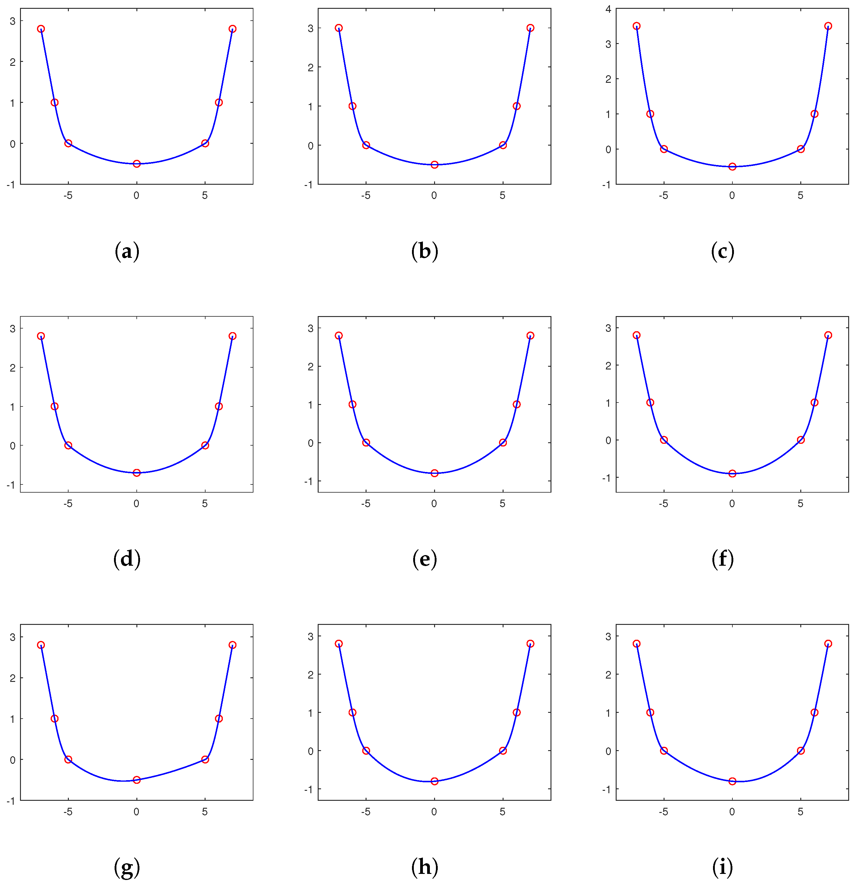
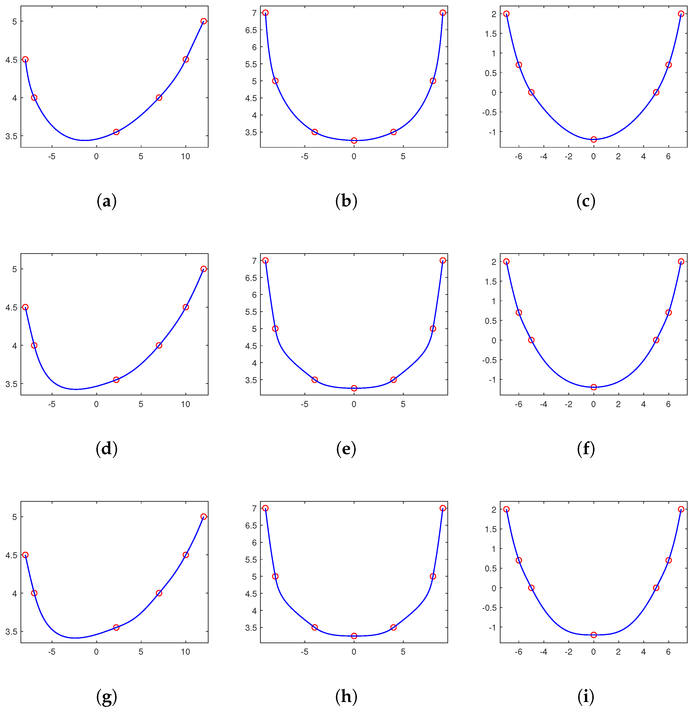
2.1. Convexity Preserving Conditions

We say that $\left\{(x_i,y_i),i=1,2,\dots ,n\right\}$ is a convex data set if and only if the slopes ${\tau }_i$, $i=1,2,\dots ,n-1$ satisfy

$$\begin{array}{c}\hfill {\tau }_1\le {\tau }_2\le \dots \le {\tau }_{n-1}.\end{array}$$

(6)

Assume that the slopes ${\tau }_1,{\tau }_2,\dots ,{\tau }_{n-1}$ satisfy (6). For $x\in [x_i,x_{i+1}]$, from (1), by direct computation, we have

$$\begin{array}{c}\hfill S^{\prime \prime }\left(x\right)={\displaystyle \frac{2p_i{\mu }_i^2}{h_i{\left[{\lambda }_{i}t+{\mu }_i(1-t)\right]}^3}},\end{array}$$

(7)

where $t=(x-x_i)/h_i\in [0,1]$. From (7), we can see that $S^{\prime \prime }\left(x\right)\ge 0$ if and only if $p_i\ge 0$. Furthermore, from (2), we can immediately obtain the following theorem.

Theorem 1.

For the points $(x_i,y_i)$, $i=1,2,\dots ,n$ in convex position, the interpolant $S\left(x\right)$ with ${\lambda }_i>0$ and ${\mu }_i>0$ is convex on $[a,b]$ if and only if

$$\begin{array}{c}\hfill m_i\le {\tau }_i,i=1,2,\dots ,n-1.\end{array}$$

(8)

From Theorem 1 and with regard to the conditions (4), the following problem arises: are there derivatives $m_i$, $i=1,2,\dots ,n$ such that

$$\begin{array}{c}\hfill \left\{\begin{array}{c}{\alpha }_i{m}_i+{\beta }_i{m}_{i+1}={\tau }_i,\hfill \\ m_i\le {\tau }_i,\hfill \end{array}\right.\end{array}$$

(9)

hold for all $1\le i\le n-1$.

For solving problem (9), we set $v_i={\tau }_i-m_i$. Then, from (4), we have

$$\begin{array}{cc}\hfill v_{i+1}& ={\tau }_{i+1}-m_{i+1}\hfill \\ \hfill & ={\tau }_{i+1}-{\tau }_i-{\displaystyle \frac{{\alpha }_i{v}_i}{{\beta }_i}},\hfill \end{array}$$

and with ${\gamma }_1=1$ and ${\delta }_1={\tau }_1$, we obtain

$$\begin{array}{c}\hfill \left\{\begin{array}{c}{\gamma }_{i+1}={\beta }_i{\gamma }_i/{\alpha }_i,i\ge 1,\hfill \\ {\delta }_{i+1}={\delta }_i+{(-1)}^i{\gamma }_{i+1}({\tau }_{i+1}-{\tau }_i),i\ge 1.\hfill \end{array}\right.\end{array}$$

(10)

It follows immediately by induction that the following equation

$$\begin{array}{c}\hfill v_i={\tau }_i-m_i={(-1)}^i(m_1-{\delta }_i)/{\gamma }_i,i\ge 1\end{array}$$

(11)

holds. Therefore, since ${\gamma }_i>0$, the requirement $v_i\ge 0$ holds for all $1\le i\le n-1$ and is equivalent to

$$\begin{array}{c}\hfill \left\{\begin{array}{c}{m}_1\ge {\delta }_i,foriisevenand1\le i\le n,\hfill \\ m_1\le {\delta }_i,foriisoddand1\le i\le n.\hfill \end{array}\right.\end{array}$$

(12)

We further set

$$\begin{array}{c}\hfill \left\{\begin{array}{c}{\delta }_{*}=max\left\{{\delta }_i:iisevenand1\le i\le n\right\},\hfill \\ {\delta }^{*}=min\left\{{\delta }_i:iisoddand1\le i\le n\right\}.\hfill \end{array}\right.\end{array}$$

(13)

Then, from (12), we can see that if ${\delta }_{*}\le {\delta }^{*}$ is satisfied, there belongs a convexity-preserving interpolation spline to every $m_1\in \left[{\delta }_{*},{\delta }^{*}\right]$. Summarizing this, the following theorem results.

Theorem 2.

For the points $(x_i,y_i)$, $i=1,2,\dots ,n$ in a convex position, there exists a convexity-preserving interpolation spline $S\left(x\right)$ if and only if the following condition holds

$$\begin{array}{c}\hfill {\delta }_{*}\le {\delta }^{*},\end{array}$$

(14)

where the numbers ${\delta }_{*}$, ${\delta }^{*}$ are defined by (10) and (13).

For a strict convex data set, that is ${\tau }_1<{\tau }_2<\dots <{\tau }_{n-1}$, we further show that there always exist parameters ${\lambda }_i>0,{\mu }_i>0,i=1,2,\dots ,n-1$ such that ${\delta }_{*}<{\delta }^{*}$ is always valid.

In fact, take i is an even number, for example. We can always choose the parameters ${\lambda }_i$, ${\mu }_i$ in such a manner that

$$\begin{array}{c}\hfill {\delta }_2<{\delta }_4<\dots <{\delta }_i<{\delta }_{i-1}<\dots <{\delta }_3<{\delta }_1.\end{array}$$

In fact, in view of (10) and of ${\alpha }_i\to 1,{\beta }_i\to 0$ for ${\lambda }_i\to +\infty$, the desired inequality

$$\begin{array}{c}\hfill {\delta }_i<{\delta }_{i+1}<{\delta }_{i-1}\end{array}$$

is always met for a sufficiently large ${\lambda }_i$.

We can thus conclude the following theorem.

Theorem 3.

Let ${\lambda }_i>0,{\mu }_i>0,i=1,2,\dots ,n-1$ be fixed, and assume (6) holds. Then, one always obtains

$$\begin{array}{c}\hfill {\delta }_{*}\le {\delta }^{*}forn\le 3,\end{array}$$

(15)

and in at least one case,

$$\begin{array}{c}\hfill {\delta }_{*}>{\delta }^{*}forn\ge 4.\end{array}$$

(16)

Proof. 

Indeed, from (10), we have ${\delta }_2\le {\delta }_1$ and ${\delta }_2\le {\delta }_3$. This implies (15). Furthermore, since ${\epsilon }_3\le {\epsilon }_4$ is valid, there are slopes ${\tau }_1,{\tau }_2,{\tau }_3,$ and ${\tau }_4$ such that ${\delta }_2\le {\delta }_1<{\delta }_4\le {\delta }_3$. In these cases, inequality (16) is obtained for all $n\ge 4$. □

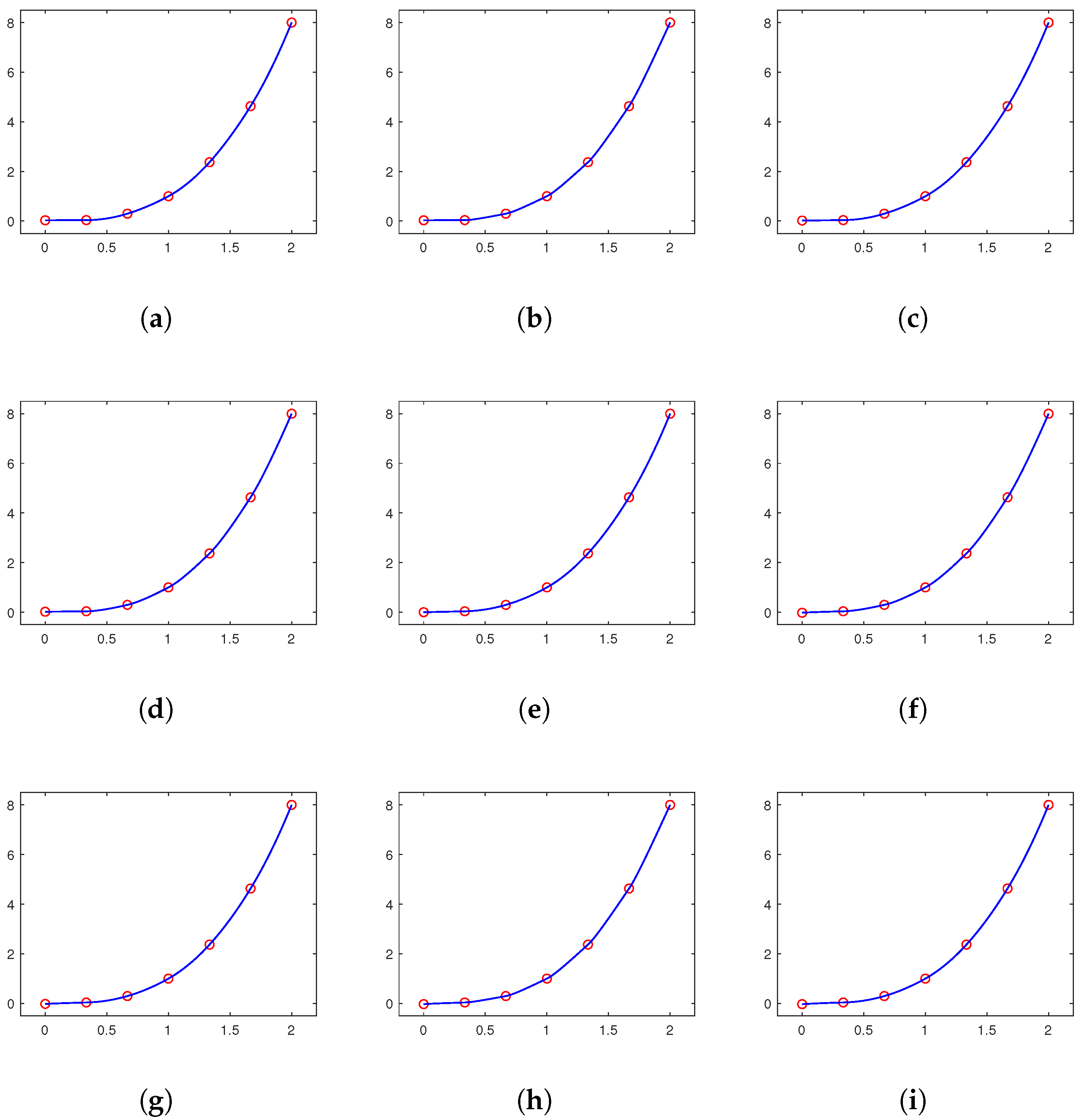
2.2. Monotonicity Preserving Conditions

We say that $\left\{(x_i,y_i),i=1,2,\dots ,n\right\}$ is a monotone increasing data set if and only if

$$\begin{array}{c}\hfill {\tau }_i\ge 0,foralli=1,2,\dots ,n-1.\end{array}$$

(17)

Now, let the given slopes ${\tau }_1,{\tau }_2,\dots ,{\tau }_{n-1}$ satisfy (17). For $x\in [x_i,x_{i+1}]$, $t=(x-x_i)/h_i$, direct computation gives that

$$\begin{array}{c}\hfill S^{\prime }\left(x\right)=m_i+{\displaystyle \frac{{\lambda }_i{t}^2+2{\mu }_{i}t-{\mu }_i{t}^2}{{\left[{\lambda }_{i}t+{\mu }_i(1-t)\right]}^2}}{p}_i.\end{array}$$

(18)

From this, together with the conditions given in (4), we can obtain the following theorem.

Theorem 4.

With all ${\lambda }_i>0$ and ${\mu }_i>0$, $S^{\prime }\left(x\right)\ge 0$ holds for any $x\in [a,b]$ if and only if the following conditions hold

$$\begin{array}{c}\hfill m_i\ge 0,i=1,2,\dots ,n.\end{array}$$

(19)

Proof. 

In fact, it suffices to verify that for any $x\in [x_i,x_{i+1}]$, $t=(x-x_i)/h_i\in [0,1]$,

$$\begin{array}{c}\hfill S^{\prime }\left(x\right)=m_i+{\displaystyle \frac{{\lambda }_i{t}^2+2{\mu }_{i}t-{\mu }_i{t}^2}{{\left[{\lambda }_{i}t+{\mu }_i(1-t)\right]}^2}}{p}_i\ge 0\end{array}$$

holds if $S^{\prime }\left(x_i\right)=m_i\ge 0$ and $S^{\prime }\left(x_{i+1}\right)=m_{i+1}\ge 0$. Indeed, from (2) and (4), $m_i\ge 0$ and $m_{i+1}\ge 0$ implies that

$$\begin{array}{cc}\hfill p_i& ={\lambda }_i({\tau }_i-m_i)\hfill \\ \hfill & \ge {\lambda }_i({\alpha }_i{m}_i-m_i)\hfill \\ \hfill & =-{\displaystyle \frac{{\lambda }_i^2{m}_i}{{\lambda }_i+{\mu }_i}}.\hfill \end{array}$$

And thus, for $0\le t\le 1$, we have

$$\begin{array}{cc}\hfill S^{\prime }\left(x\right)\ge & m_i-m_i{\displaystyle \frac{{\lambda }_i^2}{{\lambda }_i+{\mu }_i}}·{\displaystyle \frac{{\lambda }_i{t}^2+2{\mu }_{i}t-{\mu }_i{t}^2}{{\left[{\lambda }_{i}t+{\mu }_i(1-t)\right]}^2}}\hfill \\ \hfill =& m_i{\displaystyle \frac{{\lambda }_i{\mu }_i^2(1-t^2)+{\mu }_i^3{(1-t)}^2}{{\left[{\lambda }_{i}t+{\mu }_i(1-t)\right]}^2({\lambda }_i+{\mu }_i)}}\ge 0.\hfill \end{array}$$

These imply the theorem. □

In view of Theorem 4 and the conditions given in (4), one is now led to the following problem: are there derivatives $m_i$, $i=1,2,\dots ,n$ such that

$$\begin{array}{c}\hfill \left\{\begin{array}{c}{\alpha }_i{m}_i+{\beta }_i{m}_{i+1}={\tau }_i,\hfill \\ m_i\ge 0,m_{i+1}\ge 0,\hfill \end{array}\right.\end{array}$$

(20)

hold for all $1\le i\le n-1$.

For treating (20), we define ${\epsilon }_1=0$, ${\gamma }_1=1$, and

$$\begin{array}{c}\hfill \left\{\begin{array}{c}{\epsilon }_{i+1}={\epsilon }_i+{(-1)}^{i+1}{\gamma }_i{\tau }_i/{\alpha }_i,\hfill \\ {\gamma }_{i+1}={\beta }_i{\gamma }_i/{\alpha }_i,i\ge 1.\hfill \end{array}\right.\end{array}$$

(21)

By induction, we can easily obtain the following relation

$$\begin{array}{c}\hfill m_i={(-1)}^{i+1}(m_1-{\epsilon }_i)/{\gamma }_i,i\ge 1.\end{array}$$

(22)

Therefore, $m_i\ge 0$, $i=1,2,3,\dots ,n$ are equivalent to

$$\begin{array}{c}\hfill \left\{\begin{array}{c}{m}_1\ge {\epsilon }_i,foriisoddand1\le i\le n,\hfill \\ m_1\le {\epsilon }_i,foriisevenand1\le i\le n.\hfill \end{array}\right.\end{array}$$

(23)

And with the following notations

$$\begin{array}{c}\hfill \left\{\begin{array}{c}{\epsilon }_{*}=max\left\{{\epsilon }_i:iisoddand1\le i\le n\right\},\hfill \\ {\epsilon }^{*}=min\left\{{\epsilon }_i:iisevenand1\le i\le n\right\},\hfill \end{array}\right.\end{array}$$

(24)

we can obtain the following existence theorem.

Theorem 5.

Under the assumption (17), there exists a monotone increasing interpolation spline $S\left(x\right)$ if and only if

$$\begin{array}{c}\hfill {\epsilon }_{*}\le {\epsilon }^{*},\end{array}$$

(25)

with ${\epsilon }_{*}$ and ${\epsilon }^{*}$ given by (21) and (24).

For strictly monotone increasing data points, that is ${\tau }_1>0,{\tau }_2>0,\dots ,{\tau }_{n-1}>0$, we further show that there always exist parameters ${\lambda }_i>0,{\mu }_i>0,i=1,2,\dots ,n-1$ such that ${\epsilon }_{*}<{\epsilon }^{*}$ is always valid.

In fact, take i is an odd number, for example. We can always choose the parameters ${\lambda }_i$, ${\mu }_i$ in such a manner that

$$\begin{array}{c}\hfill {\epsilon }_1<{\epsilon }_3<\dots <{\epsilon }_i<{\epsilon }_{i-1}<\dots <{\epsilon }_4<{\epsilon }_2.\end{array}$$

In fact, in view of (21) and of ${\alpha }_i\to 1,{\beta }_i\to 0$ for ${\lambda }_i\to +\infty$, the desired inequality

$$\begin{array}{c}\hfill {\epsilon }_i<{\epsilon }_{i+1}<{\epsilon }_{i-1}\end{array}$$

is always met for a sufficiently large ${\lambda }_i$. We can thus conclude the follow theorem.

Theorem 6.

Let ${\lambda }_i>0,{\mu }_i>0,i=1,2,\dots ,n-1$ be fixed, and suppose (17). Then, one always has

$$\begin{array}{c}\hfill {\epsilon }_{*}\le {\epsilon }^{*}forn\le 3\end{array}$$

(26)

and in at least one case,

$$\begin{array}{c}\hfill {\epsilon }_{*}>{\epsilon }^{*}forn\ge 4.\end{array}$$

(27)

Proof. 

In fact, from (21), we have ${\epsilon }_1\le {\epsilon }_2$, ${\epsilon }_3\le {\epsilon }_2$. This implies (26). Furthermore, since ${\epsilon }_1\le {\epsilon }_2$, ${\epsilon }_3\le {\epsilon }_4$, in these cases, inequality (16) is obtained for all $n\ge 4$. □

If the data set is increasing and convex, that is

$$\begin{array}{c}\hfill 0\le {\tau }_1\le {\tau }_2\le \dots \le {\tau }_{n-1},\end{array}$$

(28)

then there exists interpolation spline $S\left(x\right)$, which is also increasing and convex, if and only if

$$\begin{array}{c}\hfill max\left\{{\delta }^{*},{\epsilon }_{*}\right\}\le min\left\{{\delta }^{*},{\epsilon }^{*}\right\}.\end{array}$$

(29)

Moreover, condition (29) can be satisfied with sufficiently large parameters ${\lambda }_i>0$, $i=1,2,\dots ,n-1$ if strong inequalities hold in (28).

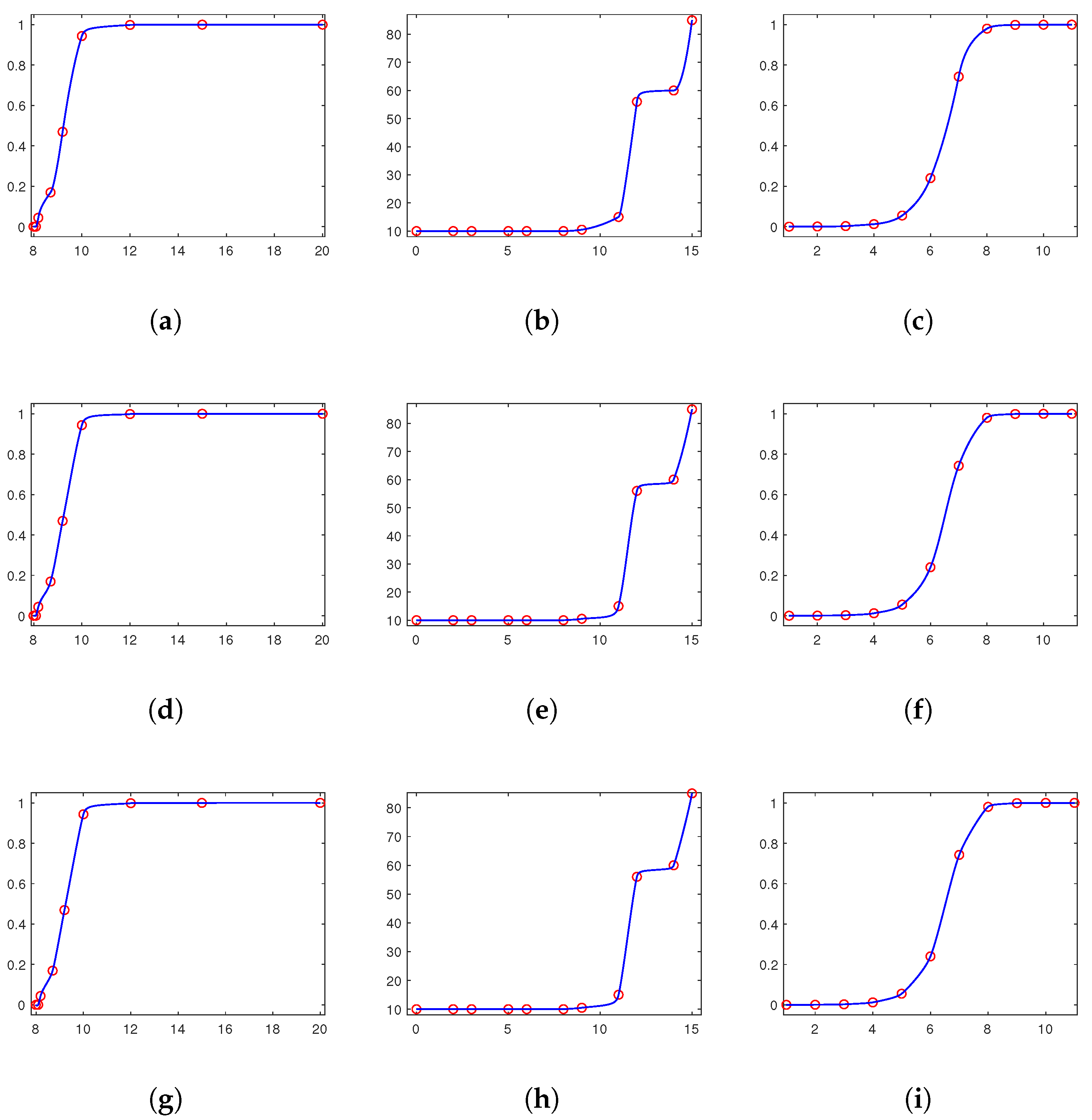
2.3. Positivity-Preserving Conditions

We say that $\left\{(x_i,y_i),i=1,2,\dots ,n\right\}$ is a non-negative data set if and only if $y_i$, $i=1,2,\dots ,n$ satisfy

$$\begin{array}{c}\hfill y_i\ge 0,i=1,2,\dots ,n.\end{array}$$

(30)

For $x\in [x_i,x_{i+1}]$ with $t=(x-x_i)/h_i$, from (1), we have

$$\begin{array}{c}\hfill \left[{\lambda }_{i}t+{\mu }_i(1-t)\right]S\left(x\right)=A_{i}t(1-t)+B_i{\left(t-C_i/\phantom{C_i{B}_i}{B}_i\right)}^2,\end{array}$$

where

$$\begin{array}{cc}\hfill A_i& ={\mu }_i{m}_i{h}_i+({\mu }_i+{\lambda }_i)y_i+2\sqrt{{\lambda }_i{\mu }_i{y}_i{y}_{i+1}},\hfill \\ \hfill B_i& ={\mu }_i{y}_i+{\lambda }_i{y}_{i+1}+2\sqrt{{\lambda }_i{\mu }_i{y}_i{y}_{i+1}},\hfill \\ \hfill C_i& ={\mu }_i{y}_i+\sqrt{{\lambda }_i{\mu }_i{y}_i{y}_{i+1}}\ge 0.\hfill \end{array}$$

Since $0\le C_i/B_i\le 1$ and ${\lambda }_{i}t+{\mu }_i(1-t)\ge 0$, from [24], we can see that the non-negative of $S\left(x\right)$ on $[x_i,x_{i+1}]$ is equivalent to $A_i\ge 0$. Thus, we can obtain the following theorem.

Theorem 7.

The rational quadratic spline interpolant $S\left(x\right)$ is non-negative on $[a,b]$ if and only if

$$\begin{array}{c}\hfill m_i\ge {\eta }_i,i=1,2,\dots ,n-1,\end{array}$$

(31)

where

$$\begin{array}{c}\hfill {\eta }_i=-{\displaystyle \frac{({\mu }_i+{\lambda }_i)y_i+2\sqrt{{\lambda }_i{\mu }_i{y}_i{y}_{i+1}}}{{\mu }_i{h}_i}}.\end{array}$$

(32)

From (7) and with regard to the conditions given in (4), the following problem arises: are there derivatives $m_i$, $i=1,2,\dots ,n$ such that

$$\begin{array}{c}\hfill \left\{\begin{array}{c}{\alpha }_i{m}_i+{\beta }_i{m}_{i+1}={\tau }_i,\hfill \\ m_i\ge {\eta }_i,\hfill \end{array}\right.\end{array}$$

(33)

hold for all $1\le i\le n-1$.

For treating (33), we define $d_1={\eta }_1,c_1=1$ and

$$\begin{array}{c}\hfill \left\{\begin{array}{c}{d}_{i+1}=d_i+{(-1)}^i{c}_i\left[{\displaystyle \frac{{\lambda }_i}{{\mu }_i}}{\eta }_{i+1}+{\eta }_i-(1+{\displaystyle \frac{{\lambda }_i}{{\mu }_i}}){\tau }_i\right],\hfill \\ c_{i+1}={\displaystyle \frac{{\lambda }_i}{{\mu }_i}}{c}_i,\hfill \end{array}\right.\end{array}$$

(34)

where $i=1,2,\dots ,n-1$.

From (4), we can easily verify that

$$\begin{array}{c}\hfill m_i-{\eta }_i={(-1)}^i{\displaystyle \frac{d_i-m_1}{c_i}},i=1,2,\dots ,n-1.\end{array}$$

(35)

Hence, condition (31) reads as

$$\begin{array}{c}\hfill \left\{\begin{array}{c}{m}_1\le d_i,foriisevenand1\le i\le n,\hfill \\ m_1\ge d_i,foriisoddand1\le i\le n.\hfill \end{array}\right.\end{array}$$

Thus, by setting

$$\begin{array}{c}\hfill \left\{\begin{array}{c}{d}^{*}=min\left\{d_i:iisevenand1\le i\le n\right\},\hfill \\ d_{*}=max\left\{d_i:iisoddand1\le i\le n\right\},\hfill \end{array}\right.\end{array}$$

(36)

we can easily obtain the following theorem.

Theorem 8.

For the non-negative data set $\left\{(x_i,y_i),i=1,2,\dots ,n\right\}$, the interpolant $S\left(x\right)$ with ${\lambda }_i>0$ and ${\mu }_i>0$ is non-negative on $[a,b]$ if and only if

$$\begin{array}{c}\hfill d_{*}\le d^{*}.\end{array}$$

(37)

For all $y_i>0$, we further show that there always exist parameters ${\lambda }_i>0,{\mu }_i>0,$$i=1,2,\dots ,n-1$ such that $d_{*}<d^{*}$ is always valid.

In fact, since ${\eta }_i\to -\infty$ for ${\lambda }_i\to +\infty$, for a sufficiently large ${\lambda }_i$, $i=1,2,\dots ,n-1$, it follows that

$$\begin{array}{c}\hfill \dots d_3\le d_1<d_2\le d_4\dots ,\end{array}$$

and therefore, the condition (37) is satisfied. Thus, we have the following theorem.

Theorem 9.

For $y_i>0$, $i=1,2,\dots ,n$. Then, for sufficiently large parameters ${\lambda }_i$, $i=1,2,\dots ,n$, the interpolant $S\left(x\right)$ is non-negative on $[a,b]$.

3. Adaptive Choice of Shape-Preserving Interpolation Splines

From the above Theorems 2, 5 and 8, we can see that convexity-, monotonicity- or non-negativity-preserving interpolants $S\left(x\right)$ are uniquely solvable only for ${\delta }_{*}={\delta }^{*}$, ${\epsilon }_{*}={\epsilon }^{*}$ or $d_{*}=d^{*}$, respectively. Furthermore, for ${\delta }_{*}<{\delta }^{*}$, ${\epsilon }_{*}<{\epsilon }^{*}$ or $d_{*}<d^{*}$, there exists an infinite number of convexity-, monotonicity- or non-negativity-preserving interpolants $S\left(x\right)$. In this section, we shall minimize a particular approximated curvature to select a visually appealing shape-preserving interpolation spline.

The classical geometric curvature is defined as follows

$$\begin{array}{c}\hfill {\int }_a^b{\displaystyle \frac{S^{\prime \prime }{\left(x\right)}^2}{{\left[1+S^{\prime }{\left(x\right)}^2\right]}^3}}dx,\end{array}$$

(38)

which is usually used as an objective function, while in real applications, the denominator makes the integration a big difficulty. In order to obtain a more convenient objective function, we follow the method given in [24] to approximate $S^{\prime }\left(x\right)$ by the slope ${\tau }_i$ given in (3) for $x_i\le x\le x_{i+1}$. Therefore, the following particular approximated curvature is taken as the objective function for selecting a shape-preserving interpolation spline

$$\begin{array}{cc}\hfill C\left(S\right)& =\sum _{i=1}^{n-1}{w}_i{\int }_{x_i}^{x_{i+1}}{S}^{\prime \prime }{\left(x\right)}^{2}dx\hfill \\ \hfill & =\sum _{i=1}^{n-1}{R}_i{({\tau }_i-m_i)}^2,\hfill \end{array}$$

(39)

with

$$\begin{array}{c}\hfill R_i={\displaystyle \frac{4w_i({\mu }_i^4+{\mu }_i^3{\lambda }_i+{\mu }_i^2{\lambda }_i^2+{\mu }_i{\lambda }_i^3+{\lambda }_i^4)}{5h_i{\lambda }_i^3{\mu }_i}}\end{array}$$

(40)

where $w_i=1/{(1+{\tau }_i^2)}^3$; see [24].

Thus, when dealing with a convex set of data, we use the following quadratic program to select a convexity-preserving interpolant $S\left(x\right)$

$$\begin{array}{c}\hfill \left\{\begin{array}{c}\underset{m_1}{\min }\mathrm{C}\left(\mathrm{S}\right)\hfill \\ s.t.{\delta }_{*}\le m_1\le {\delta }^{*}.\hfill \end{array}\right.\end{array}$$

(41)

Furthermore, when dealing with monotone increasing sets of data, we use the following quadratic program to select a monotonicity-preserving interpolant $S\left(x\right)$

$$\begin{array}{c}\hfill \left\{\begin{array}{c}\underset{m_1}{\min }\mathrm{C}\left(\mathrm{S}\right)\hfill \\ s.t.{\epsilon }_{*}\le m_1\le {\epsilon }^{*}.\hfill \end{array}\right.\end{array}$$

(42)

Furthermore, when dealing with a non-negative set of data, we use the following quadratic program to select a non-negativity-preserving interpolant $S\left(x\right)$

$$\begin{array}{c}\hfill \left\{\begin{array}{c}\underset{m_1}{\min }\mathrm{C}\left(\mathrm{S}\right)\hfill \\ s.t.d_{*}\le m_1\le d^{*}.\hfill \end{array}\right.\end{array}$$

(43)

The quadratic programs given in (41)–(43) are easily solved since the objective function and the constraints are actually functions of $m_1$ alone. To be more concrete, by using the relations given in (11), the quadratic program (41) reduces to

$$\begin{array}{c}\hfill \left\{\begin{array}{c}\underset{m_1}{min}{\displaystyle \sum _{i=1}^{n-1}}{\displaystyle \frac{R_i{(m_1-{\delta }_i)}^2}{{\gamma }_i^2}}\hfill \\ s.t.{\delta }_{*}\le m_1\le {\delta }^{*},\hfill \end{array}\right.\end{array}$$

(44)

and by using the relations given in (22), the quadratic program (42) reduces to

$$\begin{array}{c}\hfill \left\{\begin{array}{c}\underset{m_1}{min}{\displaystyle \sum _{i=1}^{n-1}}{\displaystyle \frac{R_i}{{\gamma }_i^2}}{\left[{\tau }_i{\gamma }_i+{(-1)}^i(m_1-{\epsilon }_i)\right]}^2\hfill \\ s.t.{\epsilon }_{*}\le m_1\le {\epsilon }^{*},\hfill \end{array}\right.\end{array}$$

(45)

and by using the relations given in (35), the quadratic program (43) reduces to

$$\begin{array}{c}\hfill \left\{\begin{array}{c}\underset{m_1}{min}{\displaystyle \sum _{i=1}^{n-1}}{\displaystyle \frac{R_i}{c_i^2}}{\left[m_1-d_i+{(-1)}^i{c}_i({\tau }_i-{\eta }_i)\right]}^2\hfill \\ s.t.d_{*}\le m_1\le d^{*}.\hfill \end{array}\right.\end{array}$$

(46)

Let the unconstrained minimizers of (44)–(46) be denoted as $m_1^{*}$, $m_1^{**}$ and $m_1^{***}$, respectively, i.e.,

$$\begin{array}{c}\hfill m_1^{*}={\displaystyle \frac{{\displaystyle \sum _{i=1}^{n-1}}\frac{R_i{\delta }_i}{{\gamma }_i^2}}{{\displaystyle \sum _{i=1}^{n-1}}\frac{R_i}{{\gamma }_i^2}}},\end{array}$$

(47)

$$\begin{array}{c}\hfill m_1^{**}={\displaystyle \frac{{\displaystyle \sum _{i=1}^{n-1}}\frac{R_i}{{\gamma }_i^2}\left[{(-1)}^{i+1}{\tau }_i{\gamma }_i+{\epsilon }_i\right]}{{\displaystyle \sum _{i=1}^{n-1}}\frac{R_i}{{\gamma }_i^2}}},\end{array}$$

(48)

$$\begin{array}{c}\hfill m_1^{***}={\displaystyle \frac{{\displaystyle \sum _{i=1}^{n-1}}\frac{R_i}{c_i^2}\left[d_i-{(-1)}^i{c}_i({\tau }_i-{\eta }_i)\right]}{{\displaystyle \sum _{i=1}^{n-1}}\frac{R_i}{c_i^2}}}.\end{array}$$

(49)

Summarizing the above discuss, we can conclude the following theorem.

Theorem 10.

The optimal minimizers $m_1^c$, $m_1^m$, and $m_1^p$ of the programs (44), (45), and (46), respectively, are given by

$$\begin{array}{c}\hfill m_1^c=\left\{\begin{array}{c}{m}_1^{*},for{\delta }_{*}\le m_1^{*}\le {\delta }^{*},\hfill \\ {\delta }^{*},for{m}_1^{*}>{\delta }^{*},\hfill \\ {\delta }_{*},for{m}_1^{*}<{\delta }_{*},\hfill \end{array}\right.\end{array}$$

(50)

$$\begin{array}{c}\hfill m_1^m=\left\{\begin{array}{c}{m}_1^{**},for{\epsilon }_{*}\le m_1^{**}\le {\epsilon }^{*},\hfill \\ {\epsilon }^{*},for{m}_1^{**}>{\epsilon }^{*},\hfill \\ {\epsilon }_{*},for{m}_1^{**}<{\epsilon }_{*},\hfill \end{array}\right.\end{array}$$

(51)

$$\begin{array}{c}\hfill m_1^p=\left\{\begin{array}{c}{m}_1^{***},for{d}_{*}\le m_1^{***}\le d^{*},\hfill \\ d^{*},for{m}_1^{***}>d^{*},\hfill \\ d_{*},for{m}_1^{***}<d_{*},\hfill \end{array}\right.\end{array}$$

(52)

where $m_1^{*}$, $m_1^{**}$, and $m_1^{***}$ are given in (47), (48), and (49), respectively.

4. Numerical Examples

Example 1.

In this example, we consider the convex data set given in

Table 1. The convex data set given in [25].

i	1	2	3	4	5	6	7
$x_i$	−7	−6	−5	0	5	6	7
$y_i$	M	1	0	$\theta$	0	1	M

. For different values of M and θ, we show the choices of ${\lambda }_i$ and ${\mu }_i$ and the corresponding optimal minimizers $m_1^c$ given in (50) in

Table 2. The optimal minimizers $m_1^c$ given by (50) for the convex data set given in Table 1.

Cases	$\mathit{\theta }$	M	${\mathit{\lambda }}_{\mathit{i}}$	${\mathit{\mu }}_{\mathit{i}}$	${\mathit{\delta }}_{*}$	${\mathit{\delta }}^{*}$	${\mathit{m}}_1^{*}$	${\mathit{m}}_1^{\mathit{c}}$
$\left(1\right)$	$-0.50$	$2.80$	$1.00$	$1.00$	$-1.8000$	$-1.8000$	$-1.8000$	$-1.8000$
$\left(2\right)$	$-0.50$	$3.00$	$1.00$	$1.00$	$-2.3000$	$-2.1000$	$-2.2000$	$-2.2000$
$\left(3\right)$	$-0.50$	$3.50$	$1.00$	$1.00$	$-3.3000$	$-3.1000$	$-3.2000$	$-3.2000$
$\left(4\right)$	$-0.70$	$2.80$	$1.00$	$1.00$	$-1.9600$	$-1.8000$	$-1.8800$	$-1.8800$
$\left(5\right)$	$-0.80$	$2.80$	$1.00$	$1.00$	$-2.0400$	$-1.8000$	$-1.9200$	$-1.9200$
$\left(6\right)$	$-0.90$	$2.80$	$1.00$	$1.00$	$-2.0400$	$-1.8000$	$-1.9600$	$-1.9600$
$\left(7\right)$	$-0.50$	$2.80$	$1.10$	$1.00$	$-1.8279$	$-1.8000$	$-1.7908$	$-1.8000$
$\left(8\right)$	$-0.80$	$2.80$	$1.10$	$1.00$	$-2.0895$	$-1.8000$	$-1.9237$	$-1.9237$
$\left(9\right)$	$-0.80$	$2.80$	$1.00$	$1.10$	$-1.9965$	$-1.8331$	$-1.9266$	$-1.9266$

. Figure 1 shows the corresponding convexity-preserving interpolation curves for different cases. From the results, we can see that the convexity-preserving interpolation curves preserve the shape of the different cases of convex data sets well.

Example 2.

In this example, we consider the monotone increasing data set given in

Table 3. Monotone increasing data set.

i	1	2	3	4	5	6	7
$x_i$	0	0.3333	0.6667	1.0000	1.3333	1.6667	2.0000
$y_i$	$\theta$	0.0370	0.2963	$1.0000$	2.3704	4.6296	8.0000

. For different values of θ, we show the choices of ${\lambda }_i$ and ${\mu }_i$ and the corresponding optimal minimizers $m_1^m$ given by (51) in

Table 4. Optimal minimizers $m_1^m$ given by (51) for the monotone increasing data set given in Table 3.

Cases	$\mathit{\theta }$	${\mathit{\lambda }}_{\mathit{i}}$	${\mathit{\mu }}_{\mathit{i}}$	${\mathit{\epsilon }}_{*}$	${\mathit{\epsilon }}^{*}$	${\mathit{m}}_1^{**}$	${\mathit{m}}_1^{\mathit{c}}$
$\left(1\right)$	$0.03$	$1.00$	$1.00$	$0.0210$	$0.0630$	$-0.1021$	$0.0210$
$\left(2\right)$	$0.03$	$4.00$	$1.00$	$0.0210$	$0.1260$	$-0.0027$	$0.0210$
$\left(3\right)$	$0.02$	$1.00$	$1.00$	$0.0510$	$0.1530$	$-0.0369$	$0.0510$
$\left(4\right)$	$0.02$	$1.00$	$0.50$	$0.0510$	$0.2040$	$0.0199$	$0.0510$
$\left(5\right)$	$0.00$	$1.00$	$1.00$	$0.1110$	$0.3330$	$0.0922$	$0.1110$
$\left(6\right)$	$-0.02$	$1.00$	$0.50$	$0.1710$	$0.6840$	$0.2686$	$0.2686$
$\left(7\right)$	$-0.02$	$1.10$	$1.00$	$0.1710$	$0.5130$	$0.2197$	$0.2197$
$\left(8\right)$	$-0.03$	$4.00$	$1.00$	$0.2010$	$1.2060$	$0.3639$	$0.3639$
$\left(9\right)$	$-0.03$	$1.00$	$1.00$	$0.2010$	$0.6030$	$0.2831$	$0.2831$

. Figure 2 shows the corresponding monotonicity-preserving interpolation curves for different cases. From the results, we can see that the monotonicity-preserving interpolation curves preserve the shape of the different cases of monotone increasing data sets well.

Example 3.

In this example, we consider the positive data set given in

Table 5. Positive data set.

i	1	2	3	4	5	6
$x_i$	1	2	3	4	5	6
$y_i$	0.1	1	$\theta$	$\theta$	1	0.1

. For different values of θ, we show the choices of ${\lambda }_i$ and ${\mu }_i$ and the corresponding optimal minimizers $m_1^p$ given by (52) in

Table 6. Optimal minimizers $m_1^p$ given by (52) for the positive data set given in Table 5.

Cases	$\mathit{\theta }$	${\mathit{\lambda }}_{\mathit{i}}$	${\mathit{\mu }}_{\mathit{i}}$	${\mathit{d}}_{*}$	${\mathit{d}}^{*}$	${\mathit{m}}_1^{***}$	${\mathit{m}}_1^{\mathit{p}}$
$\left(1\right)$	$1\times {10}^{-1}$	$1.00$	$1.00$	$3.2000$	$4.4325$	$2.8749$	$3.2000$
$\left(2\right)$	$1\times {10}^{-2}$	$1.00$	$1.00$	$3.7400$	$4.0000$	$3.0110$	$3.7400$
$\left(3\right)$	$1\times {10}^{-3}$	$1.00$	$1.00$	$3.7940$	$3.8632$	$3.0248$	$3.7940$
$\left(4\right)$	$1\times {10}^{-4}$	$1.00$	$1.00$	$3.7994$	$3.8200$	$3.0261$	$3.7994$
$\left(5\right)$	$1\times {10}^{-5}$	$1.00$	$1.00$	$3.7999$	$3.8063$	$3.0263$	$3.7999$
$\left(6\right)$	$1\times {10}^{-6}$	$1.00$	$1.00$	$3.8000$	$3.8020$	$3.0263$	$3.8000$
$\left(7\right)$	$1\times {10}^{-7}$	$1.00$	$1.00$	$3.8000$	$3.8006$	$3.0263$	$3.8000$
$\left(8\right)$	$1\times {10}^{-7}$	$1.10$	$1.00$	$4.2000$	$4.2007$	$3.2047$	$4.2000$
$\left(9\right)$	$1\times {10}^{-7}$	$1.00$	$1.10$	$3.4537$	$3.4542$	$2.8357$	$3.4537$

. Figure 3 shows the corresponding positivity-preserving interpolation curves for different cases. From the results, we can see that the positivity-preserving interpolation curves preserve the shape of the different cases of positive data sets well.

In the next three examples, we shall show some comparison between our shape-preserving interpolation splines and some existing ones.

Example 4.

In this example, we consider the convex data set given in

Table 7. Convex data set.

i	1	2	3	4	5	6
$x_i$	−8	−7	2.2	7	10	12
$y_i$	4.5	4	3.55	4	4.5	5
${\lambda }_i$	2	2	1.2	0.5	0.5	0.5
${\mu }_i$	1	1	1	1	1	1

,

Table 8. Convex data set given in [12].

i	1	2	3	4	5	6	7
$x_i$	−9	−8	−4	0	4	8	9
$y_i$	7	5	3.5	3.25	3.5	5	7
${\lambda }_i$	2	2	2	1	0.5	0.5	0.5
${\mu }_i$	1	1	1	1	1	1	1

and

Table 9. Convex data set given in [13].

i	1	2	3	4	5	6	7
$x_i$	−7	−6	−5	0	5	6	7
$y_i$	2	0.7	0	−1.2	0	0.7	2
${\lambda }_i$	1	1	1	1	1	1	1
${\mu }_i$	1	1	1	1	1	1	1

. We generate the corresponding convexity-preserving interpolation curves using the proposed method and the methods given in [12,13]. For the proposed method, the choices of parameters ${\lambda }_i$ and ${\mu }_i$ are shown in Table 7, Table 8 and Table 9. Furthermore, the corresponding numerical results of the parameters are ${\delta }^{*}=-1.1815$, ${\delta }_{*}=-0.9815$, $m_1^{**}=-0.6681$, and $m_1^m=-0.9815$ for Table 7; ${\delta }^{*}=-5$, ${\delta }_{*}=-4$, $m_1^{**}=-4.4314$, and $m_1^m=-4.4314$ for Table 8; and ${\delta }^{*}=-1.8259$, ${\delta }_{*}=-1.5117$, $m_1^{**}=-1.6512$, and $m_1^m=-1.6512$ for Table 9. From Figure 4, we can see that the convexity-preserving interpolation curves generated by the new method proposed are more attractive than those generated by the methods given in [12,13].

Example 5.

In this example, we consider the monotone increasing data set given in

Table 10. Monotone data set.

i	1	2	3	4	5	6	7	8	9
$x_i$	7.99	8.09	8.19	8.70	5	6	7	8	9
$y_i$	0	2.76429 $\times {10}^{-5}$	4.37498 $\times {10}^{-2}$	0.169183	0.469428	0.943740	0.998636	0.999916	0.999994
${\lambda }_i$	2	2	5	2	1	16.5	16.5	20	20
${\mu }_i$	1	1	1	1	1	1	1	1	1

,

Table 11. Monotone data set given in [6].

i	1	2	3	4	5	6	7	8	9	10	11
$x_i$	0	2	3	5	6	8	9	11	12	14	15
$y_i$	10	10	10	10	10	10	10.5	15	56	60	85
${\lambda }_i$	1	1	1	1	1	1	1	5	25	1	1
${\mu }_i$	1	1	1	1	1	1	10	1	1	1	1

and

Table 12. The monotone data set given in [14].

i	1	2	3	4	5	6	7	8	9	10	11
$x_i$	1	2	3	4	5	6	7	8	9	10	11
$y_i$	0.0001	0.0006	0.0027	0.0123	0.0551	0.2402	0.7427	0.9804	0.9990	0.9999	1.0000
${\lambda }_i$	0.5	0.5	0.5	0.5	0.5	0.8	3	4	4	4	4
${\mu }_i$	1	1	1	1	1	1	1	1	1	1	1

. We generate the corresponding monotonicity-preserving interpolation curves by the proposed method and the methods given in [6,14]. For the the proposed method, the choices of parameters ${\lambda }_i$ and ${\mu }_i$ are shown in Table 10, Table 11 and Table 12. Furthermore, the corresponding numerical results of the parameters are ${\epsilon }_{*}=2.7643e-04$, ${\epsilon }^{*}=0.0011$, $m_1^{**}=-0.1339$, and $m_1^m=2.7643e-04$ for Table 10; ${\epsilon }_{*}=0$, ${\epsilon }^{*}=0$, $m_1^{**}=-0.1113$, and $m_1^m=0$ for Table 11; and ${\epsilon }_{*}=0.0011$, ${\epsilon }^{*}=0.0012$, $m_1^{**}=-0.0026$, and $m_1^m=0.0011$ for Table 12. From Figure 5, we can see that the monotonicity-preserving interpolation curves generated by the new method proposed are more attractive than the ones generated by the methods given in [6,14].

Example 6.

In this example, we consider the positive data set given in

Table 13. Positive data set.

i	1	2	3	4	5	6	7
$x_i$	0	2	4	10	28	30	32
$y_i$	20.8	8.8	4.2	0.5	3.9	6.2	9.6
${\lambda }_i$	1	1	1	1	1	1	1
${\mu }_i$	1	1	1	1.7	1.2	1	1

,

Table 14. Positive data set given in [3].

i	1	2	3	4	5	6	7
$x_i$	1	2	4	5	7	8	9
$y_i$	24.6162	2.4616	41.027	4.10277	57.4378	5.7438	0.5744
${\lambda }_i$	1	1	1	1	1	1	1
${\mu }_i$	0.1	0.1	0.1	0.1	0.1	0.1	0.1

and

Table 15. Positive data set given in [5].

i	1	2	3	4	5	6	7	8	9
$x_i$	0	0.25	0.5	1	1.5	2	2.5	3	4
$y_i$	2	0.6	0.1	0.13	1	0.5	1.1	0.25	0.2
${\lambda }_i$	1	1	1	10	1	1	1	10	1
${\mu }_i$	1	1	1	1	0.5	0.7	1	0.4	0.4

. We generate the corresponding positivity-preserving interpolation curves by the proposed method and the methods given in [3,5]. For the the proposed method, the choices of parameters ${\lambda }_i$ and ${\mu }_i$ are shown in Table 13, Table 14 and Table 15. Furthermore, the corresponding numerical results of the parameters are $d_{*}=-9.2830$, $d^{*}=-8.4702$, $m_1^{***}=-8.4257$, and $m_1^p=-8.4702$ for Table 13; $d_{*}=-320.0104$, $d^{*}=209.4799$, $m_1^{***}=-29.9358$, and $m_1^p=-29.9358$ for Table 14; and $d_{*}=-8.0561$, $d^{*}=-4.4404$, $m_1^{***}=-7.8820$, $m_1^p=-7.8820$ for Table 15. From Figure 6, we can see that the positivity-preserving interpolation curves generated by the new method proposed are more attractive than those generated by the methods given in [3,5].

5. Conclusions

We have proposed a kind of $C^1$ rational quadratic interpolation spline featuring two symmetric parameters. This generalization encompasses the positivity-preserving rational quadratic spline presented in [24] as a special case. Additionally, we have derived the necessary and sufficient conditions for ensuring that the interpolant preserves convexity, monotonicity, and positivity. To enhance the visual appeal of the resulting shape-preserving interpolation curves, we have introduced an optimization-based approach by minimizing a particular approximated curvature metric, which enables the construction of shape-preserving interpolation splines with aesthetically pleasing characteristics. Compared with the shape-preserving methods given in [3,5,6,12,13,14], the shape-preserving interpolation curves generated by the new method proposed are more visually pleasing. Future research will extend this framework to develop shape-preserving interpolation techniques for surfaces.

References

1. Kvasov, B.I. Methods of Shape-Preserving Spline Approximation; World Scientific: Singapore, 2000. [Google Scholar]
2. Goodman, T.N.T. Shape preserving interpolation by curves. In Algorithms for Approximation IV; Leversity, J., Anderson, I., Mason, J., Eds.; University of Huddersfield: Huddersfield, UK, 2002; pp. 24–35. [Google Scholar]
3. Hussain, M.Z.; Sarfraz, M. Positivity-preserving interpolation of positive data by rational cubics. J. Comput. Appl. Math. 2008, 218, 446–458. [Google Scholar] [CrossRef]
4. Sarfraz, M.; Hussain, M.Z.; Nisar, A. Positive data modeling using spline function. Appl. Math. Comput. 2010, 216, 2036–2049. [Google Scholar] [CrossRef]
5. Qin, X.B.; Qin, L.; Xu, Q.S. C1 positive-preserving interpolation schemes with local free parameters. IAENG Int. J. Comput. Sci. 2016, 43, 1–9. [Google Scholar]
6. Gregory, J.A.; Delbourgo, R. Piecewise rational quadratic interpolation to monotonic data. IMA J. Numer. Anal. 1982, 2, 123–130. [Google Scholar] [CrossRef]
7. Sarfraz, M. A rational cubic spline for the visualization of monotonic data. Comput. Graph. 2000, 24, 509–516. [Google Scholar] [CrossRef]
8. Sarfraz, M. A rational cubic spline for the visualization of monotonic data: An alternate approach. Comput. Graph. 2003, 27, 107–121. [Google Scholar] [CrossRef]
9. Hussain, M.Z.; Hussain, M. Visualization of data preserving monotonicity. Appl. Math. Comput. 2007, 190, 1353–1364. [Google Scholar] [CrossRef]
10. Hussain, M.Z.; Sarfraz, M. Monotone piecewise rational cubic interpolation. Int. J. Comput. Math. 2009, 86, 423–430. [Google Scholar] [CrossRef]
11. Abbas, M.; Majid, A.A.; Ali, J.M. Monotonicity-preserving C2 rational cubic spline for monotone data. Appl. Math. Comput. 2012, 219, 2885–2895. [Google Scholar] [CrossRef]
12. Delbourgo, R. Shape preserving interpolation to convex data by rational functions with quadratic numerator and linear denominator. IMA J. Numer. Anal. 1989, 9, 123–136. [Google Scholar] [CrossRef]
13. Sarfraz, M.; Hussain, M.Z. Shape-preserving curve interpolation. Int. J. Comput. Math. 2012, 89, 35–53. [Google Scholar] [CrossRef]
14. Sarfraz, M.; Hussain, M.Z.; Hussain, M. Modeling rational spline for visualization of shaped data. J. Numer. Math. 2013, 21, 63–87. [Google Scholar] [CrossRef]
15. Abbas, M.; Majid, A.A.; Ali, J.M. Local convexity-preserving C2 rational cubic spline for convex data. Sci. World J. 2014, 2014, 391568. [Google Scholar] [CrossRef] [PubMed]
16. Kvasov, B.I. Monotone and convex interpolation by weighted cubic splines. Comput. Math. Math. Phys. 2003, 53, 1428–1439. [Google Scholar] [CrossRef]
17. Kvasov, B.I. Monotone and convex interpolation by weighted quadratic splines. Adv. Comput. Math. 2014, 40, 91–116. [Google Scholar] [CrossRef]
18. Kvasov, B.I. Discrete weighted cubic splines. Numer. Algor. 2014, 67, 863–888. [Google Scholar] [CrossRef]
19. Han, X.L. Convexity-preserving piecewise rational quartic interpolation. SIAM J. Numer. Anal. 2008, 46, 920–929. [Google Scholar] [CrossRef]
20. Han, X.L. Shape-preserving piecewise rational interpolant with quartic numeratror and quadratic denominator. Appl. Math. Comput. 2015, 251, 258–274. [Google Scholar]
21. Zhu, Y.P.; Han, X.L. C2 rational quartic interpolation spline with local shape preserving property. Appl. Math. Lett. 2015, 46, 57–63. [Google Scholar] [CrossRef]
22. Zhu, Y.P. C2 Rational quartic/cubic spline interpolant with shape constraints. Res. Math. 2018, 73, 73–127. [Google Scholar] [CrossRef]
23. Zhu, Y.P. C2 positivity-preserving rational interpolation splines in one and two dimensions. Appl. Math. Comput. 2018, 316, 186–204. [Google Scholar] [CrossRef]
24. Schmidt, J.W.; Hess, W. Positive Interpolation with Rational Quadratic Splines. Computing 1987, 38, 261–267. [Google Scholar] [CrossRef]
25. Schmidt, J.W.; Hess, W. Quadratic and related exponential splines in shape preserving interpolation. J. Comput. Appl. Math. 1987, 18, 321–329. [Google Scholar] [CrossRef]
Figure 1. Optimal convexity-preserving interpolation curves for the convex data set given in Table 1 with the different cases of θ , M, λ i , and μ i given in Table 2. (a) Case 1. (b) Case 2. (c) Case 3. (d) Case 4. (e) Case 5. (f) Case 6. (g) Case 7. (h) Case 8. (i) Case 9.
Symmetry 17 00815 g001
Figure 2. Optimal monotonicity-preserving interpolation curves for the monotone increasing data set given in Table 3 with the different cases of θ , λ i , and μ i given in Table 4. (a) Case 1. (b) Case 2. (c) Case 3. (d) Case 4. (e) Case 5. (f) Case 6. (g) Case 7. (h) Case 8. (i) Case 9.
Symmetry 17 00815 g002
Figure 3. Optimal positivity-preserving interpolation curves for the monotone increasing data set given in Table 5 with the different cases of θ , λ i , and μ i given in Table 6. (a) Case 1. (b) Case 2. (c) Case 3. (d) Case 4. (e) Case 5. (f) Case 6. (g) Case 7. (h) Case 8. (i) Case 9.
Symmetry 17 00815 g003
Figure 4. Comparison of the convexity-preserving interpolation curves for the convex data sets given in Table 7, Table 8, and Table 9, respectively. (a) By our method. (b) By our method. (c) By our method. (d) By the method given in [12]. (e) By the method given in [12]. (f) By the method given in [12]. (g) By the method given in [13]. (h) By the method given in [13]. (i) By the method given in [13].
Symmetry 17 00815 g004
Figure 5. Comparison of the monotonicity-preserving interpolation curves for the convex data set given in Table 10, Table 11, and Table 12, respectively. (a) By our method. (b) By our method. (c) By our method. (d) By the method given in [6]. (e) By the method given in [6]. (f) By the method given in [6]. (g) By the method given in [14]. (h) By the method given in [14]. (i) By the method given in [14].
Symmetry 17 00815 g005
Figure 6. Comparison of the monotonicity-preserving interpolation curves for the convex data set given in Table 13, Table 14, and Table 15, respectively. (a) By our method. (b) By our method. (c) By our method. (d) By the method given in [3]. (e) By the method given in [3]. (f) By the method given in [3]. (g) By the method given in [5]. (h) By the method given in [5]. (i) By the method given in [5].
Symmetry 17 00815 g006