Improved Estimator Using Auxiliary Information in Adaptive Cluster Sampling with Networks Selected Without Replacement

Abstract

Adaptive cluster sampling (ACS) is an efficient sampling technique for studying populations where the characteristic of interest is rare or spatially clustered. This method is widely applied in fields such as ecological studies, epidemiology, and resource management. ACS initially selects sampling units using simple random sampling without replacement. However, in some cases, selected networks may overlap, leading to multiple networks being included in the sample. To address this issue, a modified version of ACS was developed to ensure sampling without replacement at the network level, maintaining sampling symmetry and preventing the inclusion of overlapping networks. Despite this adjustment, asymmetry may still occur when network formation is highly irregular. This issue can be mitigated by incorporating auxiliary variables, which help correct distortions in the sampling process. In many situations, auxiliary variables related to the variable of interest can be utilized to enhance the precision of population parameter estimates. This research proposes multiplicative generalization for an estimator with two auxiliary variables using adaptive cluster sampling with networks selected without replacement. The bias and mean square error (MSE) are derived using a Taylor series expansion to determine the optimal conditions for minimizing MSE. A simulation study is conducted to support the theoretical findings. The results show that the proposed estimator under the optimal values of $T_1$ and $T_2$ is the most efficient to minimize MSE.

1. Introduction

Adaptive cluster sampling (ACS) is a data-driven method for efficiently estimating the abundance of rare and clustered populations. First introduced by Thompson in 1990 [1], ACS begins by selecting initial sample units using simple random sampling without replacement. If an initial unit satisfies a predefined condition C, its neighboring units are added to the sample. If any of those neighboring units also satisfy condition C, their respective neighborhoods are added in turn. This process continues until no additional units meet the condition. Conversely, if the initial unit does not satisfy condition C, no additional units are added, and the cluster remains a single unit. The initial set of sample units and all subsequently included neighborhoods that satisfy condition C are collectively referred to as networks. In this context, a “neighborhood” is defined as the four spatially adjacent units located at the top, bottom, left, and right (i.e., north, south, west, and east) of the selected unit (Figure 1). For instance, if a unit marked with a star is the initial selection, then the condition for adding neighboring units could be a value greater than or equal to one. The green units in the figure illustrate a single network formed under this sampling framework. Adaptive cluster sampling (ACS) has been widely utilized in various survey applications, particularly in cases where the characteristic of interest is rare or spatially clustered. Research employing ACS includes studies on forest ecosystems [2], herpetofauna in tropical rainforests [3], larvae of the sea lamprey [4], freshwater mussel populations [5], hydroa-coustic surveys [6], and assessments related to the COVID-19 pandemic [7,8,9]. Additionally, ACS has been explored in autonomous systems [10] and Internet of Things (IoT) applications [11].

Thompson proposed an unbiased estimator for ACS under the condition that units are selected without replacement. The initials were selected using simple random sampling. However, some selected networks occasionally contained more than one selected network. Building on this framework, Salehi and Seber [12] introduced ACS without replacement at the network level and developed an estimator that leveraged prior work by Des Raj and Murthy.

The estimators discussed above were primarily designed to estimate a single variable of interest. However, in many situations, other variables are closely related to the variable of interest. Leveraging auxiliary information from these related variables is a well-established method to enhance the precision of estimation. Several researchers have developed estimators for adaptive cluster sampling without replacement that incorporate auxiliary information from such variables. Chao [13] introduced a ratio estimator, while Dryver and Chao [14] proposed modified ratio estimators. Chutiman and Kumphon [15] suggested regression, difference, and modified ratio estimators. Additionally, Chutiman [16] and Yadav et al. [17] proposed ratio estimators based on population parameters, including the coefficient of variation, kurtosis, skewness, and correlations with auxiliary variables. Chaudhry and Hanif [18] introduced a generalized exponential-cum-exponential estimator utilizing network averages, whereas Singh and Mishra [19] proposed transformed ratio-type estimators. Finally, Bhat et al. [20] developed a generalized class of ratio-type estimators. Finally, Mishra et al. [21] proposed combined ratio and product-type estimators.

Chutiman and Chiangpradit [22] developed a ratio estimator that utilized auxiliary variable information for adaptive cluster sampling, with networks selected without replacement. However, their approach was limited to the use of a single auxiliary variable. To address this limitation, this paper focuses on advancing adaptive cluster sampling estimators by incorporating information from two auxiliary variables, with networks still selected without replacement. Section 2 outlines key concepts of adaptive cluster sampling without the replacement of units, while Section 3 expands on sampling without the replacement of networks. The proposed estimators for adaptive cluster sampling without the replacement of networks are introduced in Section 4, followed by simulation studies presented in Section 5. Finally, the conclusions drawn from this study are discussed in Section 6.

2. Concept of ACS Without Replacement of Units

Consider a finite population, $U=U_1,U_2,\dots ,U_N$, of size N units. Let y denote the variable of interest taking the values $y_i$ on the unit $U_i(i=1,2,\dots ,N)$, with ${\tau }_y$ representing the unknown total population of the variable of interest.

Let n denote the initial sample size and $\nu$ denote the final sample size. Let ${\psi }_i$ denote a network that includes unit i and $m_i$ as the number of units in that network. The initial sample of units is selected by simple random sampling without replacement. The Hansen–Hurwitz estimator of the total population for the variable of interest can be written as

$${\left({\widehat{\tau }}_y\right)}_{\mathrm{HH}}={\displaystyle \frac{N}{n}}\sum _{i=1}^n{\left(w_y\right)}_i,$$

(1)

where ${\left(w_y\right)}_i$ is the average of the variable of interest in the network that includes the unit of the initial sample, ${\left(w_y\right)}_i={\displaystyle \frac{1}{m_i}}{\sum }_{j\in {\psi }_i}{y}_j$.

The mean square error (MSE) of ${\left({\widehat{\tau }}_y\right)}_{HH}$ is

$$MSE{\left({\widehat{\tau }}_y\right)}_{HH}={\displaystyle \frac{N(N-n)}{(N-1)}}\sum _{i=1}^N{\left({\left(w_y\right)}_i-{\displaystyle \frac{{\tau }_y}{N}}\right)}^2.$$

(2)

When the auxiliary variable $\left(x\right)$ is available, and this auxiliary variable has a positive relationship with the variable of interest, a ratio estimator is employed to enhance the efficiency of the estimator. Dryver and Chao [14] proposed a modified ratio estimator as

$${\left({\widehat{\tau }}_y\right)}_{DC}={\displaystyle \frac{{\left({\widehat{\tau }}_y\right)}_{HH}}{{\left({\widehat{\tau }}_x\right)}_{HH}}}{\tau }_x,$$

(3)

where ${\left({\widehat{\tau }}_y\right)}_{HH}$ is the Hansen–Hurwitz estimator of the population total for the auxiliary variable and ${\tau }_x$ is the population total of the auxiliary variable. The MSE of ${\left({\widehat{\tau }}_y\right)}_{DC}$ is

$$MSE{\left({\widehat{\tau }}_y\right)}_{DC}={\displaystyle \frac{N(N-n)}{(N-1)}}\sum _{i=1}^N{\left({\left(w_y\right)}_i-R{\left(w_x\right)}_i\right)}^2,$$

(4)

where $R={\displaystyle \frac{{\tau }_y}{{\tau }_x}}$.

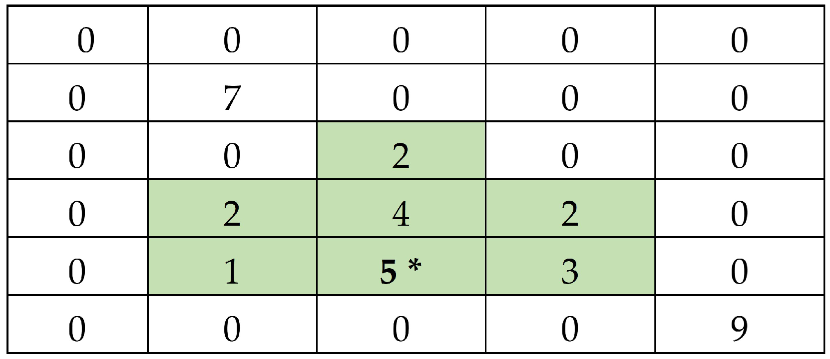
3. Concept of ACS with Networks Selected Without Replacement

In adaptive cluster sampling, the number of distinct networks selected is inherently random. It is possible for multiple initial sampled units to fall within the same network, resulting in some units being selected more than once. Salehi and Seber [12] introduced a new sampling design as an adaptive cluster sampling with networks selected without replacement.

In this approach, the first sample unit is selected using simple random sampling from the population. A network is then formed based on this unit and subsequently removed from the population. The second sample unit is selected using simple random sampling without replacement from the remaining units, and a second network is formed. This process is repeated until networks have been selected.

Let $p_i$ be the first—draw probabilities for the network that includes unit i. Thus, $p_i={\displaystyle \frac{m_i}{N}}$, where $m_i$ is the number of units in the network that includes unit i. So, $p_i/\left(1-{\sum }_{j=1}^{i-1}{p}_j\right)$ is the conditional ith draw probability for the iþnetwork, which includes the unit iþin the sample given the first $i-1$ network selection.

Building on work by Des Raj [23], Salehi and Seber [12] used a modified estimator, providing an unbiased estimator for the total population of the variable of interest as follows

$${\left({\widehat{\tau }}_y\right)}_{Raj}={\displaystyle \frac{1}{n}}\sum _{i=1}^n{\left(z_y\right)}_i,$$

(5)

where $i=1$, ${\left(z_y\right)}_1={\displaystyle \frac{y_{1.}}{p_1}},\mathrm{and}i=2,\dots ,n,{\left(z_y\right)}_i={\sum }_{j=1}^{i-1}{y}_{j.}+{\displaystyle \frac{\left(1-{\sum }_{j=1}^{i-1}{p}_j\right)y_{i.}}{p_i}}.$

The MSE of ${\left({\widehat{\tau }}_y\right)}_{Raj}$ is

$$MSE{\left({\widehat{\tau }}_y\right)}_{Raj}={\displaystyle \frac{1}{n^2}}\sum _{i=1}^{n}V{\left(z_y\right)}_i,$$

(6)

and an unbiased estimator of $MSE{\left({\widehat{\tau }}_y\right)}_{Rqj}$ is

$$MSE{\left({\widehat{\tau }}_y\right)}_{Raj}={\displaystyle \frac{1}{n(n-1)}}\sum _{i=1}^n{\left({\left(z_y\right)}_i-{\left({\widehat{\tau }}_y\right)}_{Raj}\right)}^2.$$

(7)

Meanwhile, Chutiman and Chiangpradit [22] presented a ratio estimator in adaptive cluster sampling without the replacement of networks.

$${\left({\widehat{\tau }}_y\right)}_{CC}={\displaystyle \frac{{\left({\widehat{\tau }}_y\right)}_{Raj}}{{\left({\widehat{\tau }}_x\right)}_{Raj}}}{\tau }_x,$$

(8)

where ${\left({\widehat{\tau }}_x\right)}_{Raj}$ is the estimator of the population total for the auxiliary variable.

The approximated MSE of ${\left({\widehat{\tau }}_y\right)}_{CC}$ is

$$MSE{\left({\widehat{\tau }}_y\right)}_{CC}\approx {\displaystyle \frac{1}{n^2}}\sum _{i=1}^{n}V\left(d_i\right),\mathrm{where}{d}_i={\left(z_y\right)}_i-R{\left(z_x\right)}_i.$$

(9)

4. Proposed Estimator in ACS Without Replacement of Networks

Motivated by Gupta and Shabbir [24] and Chutiman and Kumphon [15], the multiplicative generalization for the estimator of a population total can be written as

$${\left({\widehat{\tau }}_y\right)}_{pro}={\left({\widehat{\tau }}_y\right)}_{Raj}{\left[{\displaystyle \frac{{\tau }_x}{{\left({\widehat{\tau }}_x\right)}_{Raj}}}\right]}^{T_1}{\left[{\displaystyle \frac{{\tau }_u}{{\left({\widehat{\tau }}_u\right)}_{Raj}}}\right]}^{T_2},$$

(10)

where x and u are two auxiliary variables, and ${\left({\widehat{\tau }}_x\right)}_{Raj}$ and ${\left({\widehat{\tau }}_u\right)}_{Raj}$ are the estimators of the population total for the auxiliary variable x and u, respectively.

$\left(T_1,T_2\right)=(1,1),(-1,-1),(1,-1),$ and $(-1,1)$ are called ratio-type, product-type, ratio-cum-product type, and product-cum-ratio-type estimator, respectively.

Let ${\delta }_y={\displaystyle \frac{{\left({\widehat{\tau }}_y\right)}_{Raj}-{\tau }_y}{{\tau }_y}}$, ${\delta }_x={\displaystyle \frac{{\left({\widehat{\tau }}_x\right)}_{Raj}-{\tau }_x}{{\tau }_x}}$, and ${\delta }_u={\displaystyle \frac{{\left({\widehat{\tau }}_u\right)}_{Raj}-{\tau }_u}{{\tau }_u}}$; and $E\left({\delta }_y\right)=0$, $E\left({\delta }_x\right)=0$, and $E\left({\delta }_u\right)=0$. Thus, ${\left({\widehat{\tau }}_y\right)}_{pro}={\tau }_y(1+{\delta }_y){(1-{\delta }_x)}^{-T_1}{(1-{\delta }_u)}^{-T_2}$ and a Taylor series expansion of ${\left({\widehat{\tau }}_y\right)}_{pro}$ is

$${\left({\widehat{\tau }}_y\right)}_{pro}={\tau }_y\left\{1+{\delta }_y-T_1{\delta }_x-T_2{\delta }_u-T_1{\delta }_y{\delta }_x-T_2{\delta }_y{\delta }_u+T_1{T}_2{\delta }_x{\delta }_u+{\displaystyle \frac{T_1(T_1+1)}{2}}{\delta }_x^2+{\displaystyle \frac{T_2(T_2+1)}{2}}{\delta }_u^2\right\}+f\left({\delta }_i\right),$$

(11)

where $f\left({\delta }_i\right)$ is third or higher order term in ${\delta }_i$.

The approximate bias is given by

$$B{\left({\widehat{\tau }}_y\right)}_{\mathrm{pro}}\approx -T_{1}E\left({\delta }_y{\delta }_x\right)-T_{2}E\left({\delta }_y{\delta }_u\right)+T_1{T}_{2}E\left({\delta }_x{\delta }_u\right)+{\displaystyle \frac{T_1(T_1+1)}{2}}E\left({\delta }_x^2\right)+{\displaystyle \frac{T_2(T_2+1)}{2}}E\left({\delta }_u^2\right).$$

(12)

The approximate mean square error (MSE) of ${\left({\widehat{\tau }}_y\right)}_{pro}$ is

$$\begin{array}{cc}\hfill MSE{\left({\widehat{\tau }}_y\right)}_{pro}& =E{\left({\left({\widehat{\tau }}_y\right)}_{pro}-{\tau }_y\right)}^2\hfill \\ & \approx E\left[{\tau }_y^2{\left({\delta }_y-T_1{\delta }_x-T_2{\delta }_u\right)}^2\right]\hfill \\ & =E\left[{\tau }_y^2\left({\delta }_y^2+T_1^2{\delta }_x^2+T_2^2{\delta }_u^2-2T_1{\delta }_y{\delta }_x-2T_1{\delta }_y{\delta }_u+2T_1{T}_2{\delta }_x{\delta }_u\right)\right]\hfill \end{array}$$

$$MSE{\left({\widehat{\tau }}_y\right)}_{pro}={\tau }_y^2\left[E\left({\delta }_y^2\right)+T_1^{2}E\left({\delta }_x^2\right)+T_2^{2}E\left({\delta }_u^2\right)-2T_{1}E\left({\delta }_y{\delta }_x\right)-2T_{1}E\left({\delta }_y{\delta }_u\right)+2T_1{T}_{2}E\left({\delta }_x{\delta }_u\right)\right],$$

(13)

where

$$\begin{array}{cc}\hfill E\left({\delta }_y^2\right)& =V\left({\delta }_y\right)+{\left[E\left({\delta }_y\right)\right]}^2=V\left({\delta }_y\right)=V\left[{\displaystyle \frac{{\left({\widehat{\tau }}_y\right)}_{Raj}-{\tau }_y}{{\tau }_y}}\right]={\displaystyle \frac{1}{{\tau }_y^2}}V{\left({\widehat{\tau }}_y\right)}_{Raj},\hfill \\ \hfill E\left({\delta }_x^2\right)& =V\left({\delta }_x\right)+{\left[E\left({\delta }_x\right)\right]}^2=V\left({\delta }_x\right)=V\left({\displaystyle \frac{{\left({\widehat{\tau }}_x\right)}_{Raj}-{\tau }_x}{{\tau }_x}}\right)={\displaystyle \frac{1}{{\tau }_x^2}}V\left({\left({\widehat{\tau }}_x\right)}_{Raj}\right),\hfill \\ \hfill E\left({\delta }_u^2\right)& =V\left({\delta }_u\right)+{\left[E\left({\delta }_u\right)\right]}^2=V\left({\delta }_u\right)=V\left({\displaystyle \frac{{\left({\widehat{\tau }}_u\right)}_{Raj}-{\tau }_u}{{\tau }_u}}\right)={\displaystyle \frac{1}{{\tau }_u^2}}V\left({\left({\widehat{\tau }}_u\right)}_{Raj}\right),\hfill \\ \hfill E\left({\delta }_y{\delta }_x\right)& =COV({\delta }_y,{\delta }_x)+E\left({\delta }_y\right)E\left({\delta }_x\right)={\displaystyle \frac{1}{{\tau }_y{\tau }_x}}COV\left({\left({\widehat{\tau }}_y\right)}_{Raj},{\left({\widehat{\tau }}_x\right)}_{Raj}\right),\hfill \\ \hfill E\left({\delta }_y{\delta }_u\right)& =COV({\delta }_y,{\delta }_u)+E\left({\delta }_y\right)E\left({\delta }_u\right)={\displaystyle \frac{1}{{\tau }_y{\tau }_u}}COV\left({\left({\widehat{\tau }}_y\right)}_{Raj},{\left({\widehat{\tau }}_u\right)}_{Raj}\right),\hfill \\ \hfill E\left({\delta }_x{\delta }_u\right)& =COV({\delta }_x,{\delta }_u)+E\left({\delta }_x\right)E\left({\delta }_u\right)={\displaystyle \frac{1}{{\tau }_x{\tau }_u}}COV\left({\left({\widehat{\tau }}_x\right)}_{Raj},{\left({\widehat{\tau }}_u\right)}_{Raj}\right).\hfill \end{array}$$

The values of $T_1$ and $T_2$ are derived by minimizing $MSE{\left({\widehat{\tau }}_y\right)}_{pro}$ with respect to $T_1$ and $T_2$ so that ${\displaystyle \frac{\partial MSE{\left({\widehat{\tau }}_y\right)}_{pro}}{\partial T_1}}=0$ and ${\displaystyle \frac{\partial MSE{\left({\widehat{\tau }}_y\right)}_{pro}}{\partial T_2}}=0$.

$${\displaystyle \frac{\partial MSE{\left({\widehat{\tau }}_y\right)}_{pro}}{\partial T_1}}=2T_1{\tau }_y^2{\displaystyle \frac{1}{{\tau }_x^2}}V{\left({\widehat{\tau }}_x\right)}_{Raj}-2{\tau }_y^2{\displaystyle \frac{1}{{\tau }_x{\tau }_y}}COV\left({\left({\widehat{\tau }}_y\right)}_{Raj},{\left({\widehat{\tau }}_x\right)}_{Raj}\right)+2{\tau }_y^2{T}_2{\displaystyle \frac{1}{{\tau }_x{\tau }_u}}COV\left({\left({\widehat{\tau }}_x\right)}_{Raj},{\left({\widehat{\tau }}_u\right)}_{Raj}\right)=0.$$

(14)

Therefore,

$$T_1={\displaystyle \frac{COV\left({\left({\widehat{\tau }}_y\right)}_{Raj},{\left({\widehat{\tau }}_x\right)}_{Raj}\right)-T_2{R}_{uy}COV\left({\left({\widehat{\tau }}_x\right)}_{Raj},{\left({\widehat{\tau }}_u\right)}_{Raj}\right)}{R_{xy}V{\left({\widehat{\tau }}_x\right)}_{Raj}}},$$

(15)

and

$${\displaystyle \frac{\partial MSE{\left({\widehat{\tau }}_y\right)}_{pro}}{\partial T_2}}=2T_2{\tau }_y^2{\displaystyle \frac{1}{{\tau }_u^2}}V{\left({\widehat{\tau }}_u\right)}_{Raj}-2{\tau }_y^2{\displaystyle \frac{1}{{\tau }_u{\tau }_y}}COV\left({\left({\widehat{\tau }}_y\right)}_{Raj},{\left({\widehat{\tau }}_u\right)}_{Raj}\right)+2{\tau }_y^2{T}_1{\displaystyle \frac{1}{{\tau }_x{\tau }_u}}COV\left({\left({\widehat{\tau }}_x\right)}_{Raj},{\left({\widehat{\tau }}_u\right)}_{Raj}\right)=0.$$

(16)

we substitute $T_1$ from Equation (15) into Equation (16). Then, the optimum values of $T_1$ and $T_2$ are

$$T_1^{\ast }={\displaystyle \frac{COV\left({\left({\widehat{\tau }}_y\right)}_{Raj},{\left({\widehat{\tau }}_x\right)}_{Raj}\right)-T_2^{\ast }{R}_{uy}COV\left({\left({\widehat{\tau }}_x\right)}_{Raj},{\left({\widehat{\tau }}_u\right)}_{Raj}\right)}{R_{xy}V\left({\left({\widehat{\tau }}_x\right)}_{Raj}\right)}},$$

(17)

$$T_2^{\ast }={\displaystyle \frac{COV\left({\left({\widehat{\tau }}_y\right)}_{Raj},{\left({\widehat{\tau }}_u\right)}_{Raj}\right)V\left({\left({\widehat{\tau }}_x\right)}_{Raj}\right)-COV\left({\left({\widehat{\tau }}_x\right)}_{Raj},{\left({\widehat{\tau }}_u\right)}_{Raj}\right)COV\left({\left({\widehat{\tau }}_y\right)}_{Raj},{\left({\widehat{\tau }}_u\right)}_{Raj}\right)}{R_{uy}V\left({\left({\widehat{\tau }}_u\right)}_{Raj}\right)V\left({\left({\widehat{\tau }}_x\right)}_{Raj}\right)-R_{uy}{\left[COV\left({\left({\widehat{\tau }}_x\right)}_{Raj},{\left({\widehat{\tau }}_u\right)}_{Raj}\right)\right]}^2}},$$

(18)

where $R_{xy}={\displaystyle \frac{{\tau }_y}{{\tau }_x}}$ and $R_{uy}={\displaystyle \frac{{\tau }_y}{{\tau }_u}}$.

The estimators of $T_1^{\ast }$ and $T_2^{\ast }$ are

$${\widehat{T}}_1^{\ast }=\frac{\widehat{COV}\left({\left({\widehat{\tau }}_y\right)}_{Raj},{\left({\widehat{\tau }}_x\right)}_{Raj}\right)-{\widehat{T}}_2^{\ast }{\widehat{R}}_{uy}\widehat{COV}\left({\left({\widehat{\tau }}_x\right)}_{Raj},{\left({\widehat{\tau }}_u\right)}_{Raj}\right)}{{\widehat{R}}_{xy}\widehat{V}\left({\left({\widehat{\tau }}_x\right)}_{Raj}\right)},$$

(19)

$${\widehat{T}}_2^{\ast }=\frac{\widehat{COV}\left({\left({\widehat{\tau }}_y\right)}_{Raj},{\left({\widehat{\tau }}_u\right)}_{Raj}\right)\widehat{V}\left({\left({\widehat{\tau }}_x\right)}_{Raj}\right)-\widehat{COV}\left({\left({\widehat{\tau }}_x\right)}_{Raj},{\left({\widehat{\tau }}_u\right)}_{Raj}\right)\widehat{COV}\left({\left({\widehat{\tau }}_y\right)}_{Raj},{\left({\widehat{\tau }}_u\right)}_{Raj}\right)}{{\widehat{R}}_{uy}\widehat{V}\left({\left({\widehat{\tau }}_u\right)}_{Raj}\right)\widehat{V}\left({\left({\widehat{\tau }}_x\right)}_{Raj}\right)-{\widehat{R}}_{uy}{\left[\widehat{COV}\left({\left({\widehat{\tau }}_x\right)}_{Raj},{\left({\widehat{\tau }}_u\right)}_{Raj}\right)\right]}^2},$$

(20)

where ${\widehat{R}}_{xy}={\displaystyle \frac{{\left({\widehat{\tau }}_y\right)}_{Raj}}{{\left({\widehat{\tau }}_x\right)}_{Raj}}}$ and ${\widehat{R}}_{uy}={\displaystyle \frac{{\left({\widehat{\tau }}_y\right)}_{Raj}}{{\left({\widehat{\tau }}_u\right)}_{Raj}}}$,

$$\begin{array}{ccc}\hfill & \widehat{V}{\left({\widehat{\tau }}_x\right)}_{Raj}={\displaystyle \frac{1}{n(n-1)}}\sum _{i=1}^n{\left({\left(z_x\right)}_i-{\left({\widehat{\tau }}_x\right)}_{Raj}\right)}^2,\hfill & \\ \hfill & \widehat{V}{\left({\widehat{\tau }}_u\right)}_{Raj}={\displaystyle \frac{1}{n(n-1)}}\sum _{i=1}^n{\left({\left(z_u\right)}_i-{\left({\widehat{\tau }}_u\right)}_{Raj}\right)}^2,\hfill & \\ \hfill & \widehat{COV}\left({\left({\widehat{\tau }}_y\right)}_{Raj},{\left({\widehat{\tau }}_x\right)}_{Raj}\right)={\displaystyle \frac{1}{n(n-1)}}\sum _{i=1}^n\left[\left({\left(z_y\right)}_i-{\left({\widehat{\tau }}_y\right)}_{Raj}\right)\left({\left(z_x\right)}_i-{\left({\widehat{\tau }}_x\right)}_{Raj}\right)\right],\hfill & \\ \hfill & \widehat{COV}\left({\left({\widehat{\tau }}_y\right)}_{Raj},{\left({\widehat{\tau }}_u\right)}_{Raj}\right)={\displaystyle \frac{1}{n(n-1)}}\sum _{i=1}^n\left[\left({\left(z_y\right)}_i-{\left({\widehat{\tau }}_y\right)}_{Raj}\right)\left({\left(z_u\right)}_i-{\left({\widehat{\tau }}_u\right)}_{Raj}\right)\right],\hfill & \\ \hfill & \widehat{COV}\left({\left({\widehat{\tau }}_x\right)}_{Raj},{\left({\widehat{\tau }}_u\right)}_{Raj}\right)={\displaystyle \frac{1}{n(n-1)}}\sum _{i=1}^n\left[\left({\left(z_x\right)}_i-{\left({\widehat{\tau }}_x\right)}_{Raj}\right)\left({\left(z_u\right)}_i-{\left({\widehat{\tau }}_u\right)}_{Raj}\right)\right].\hfill \end{array}$$

5. Results and Discussion

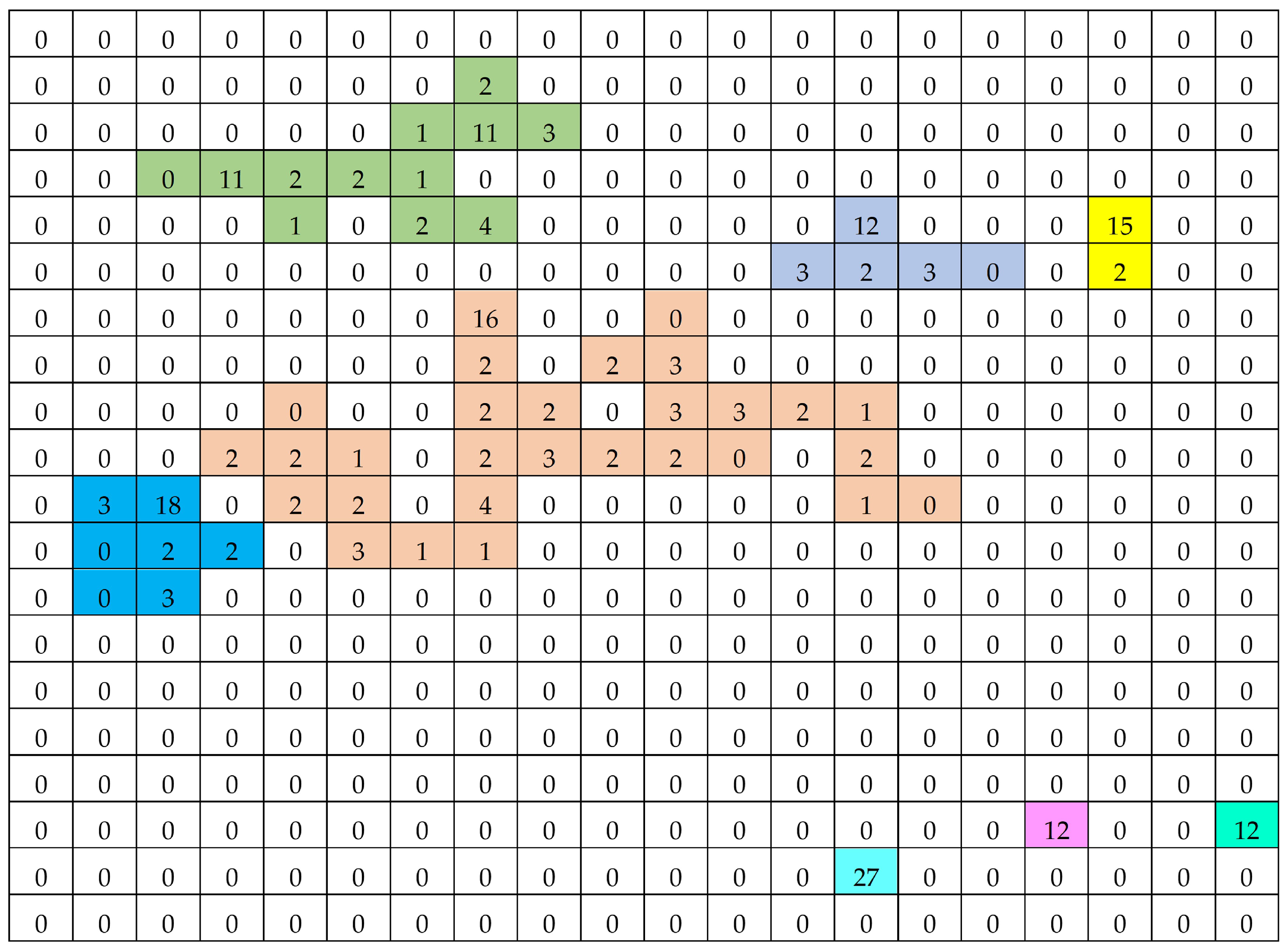
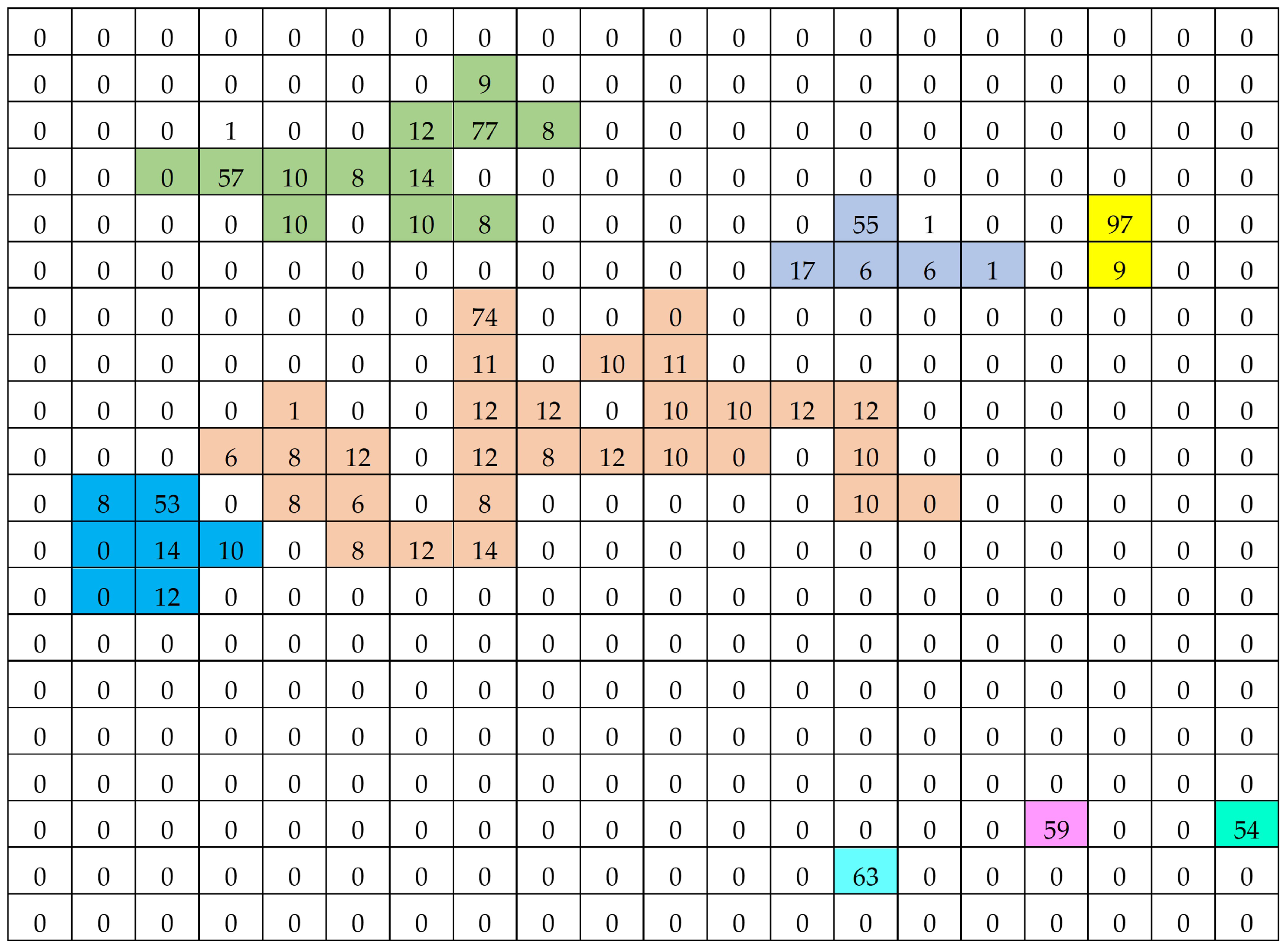
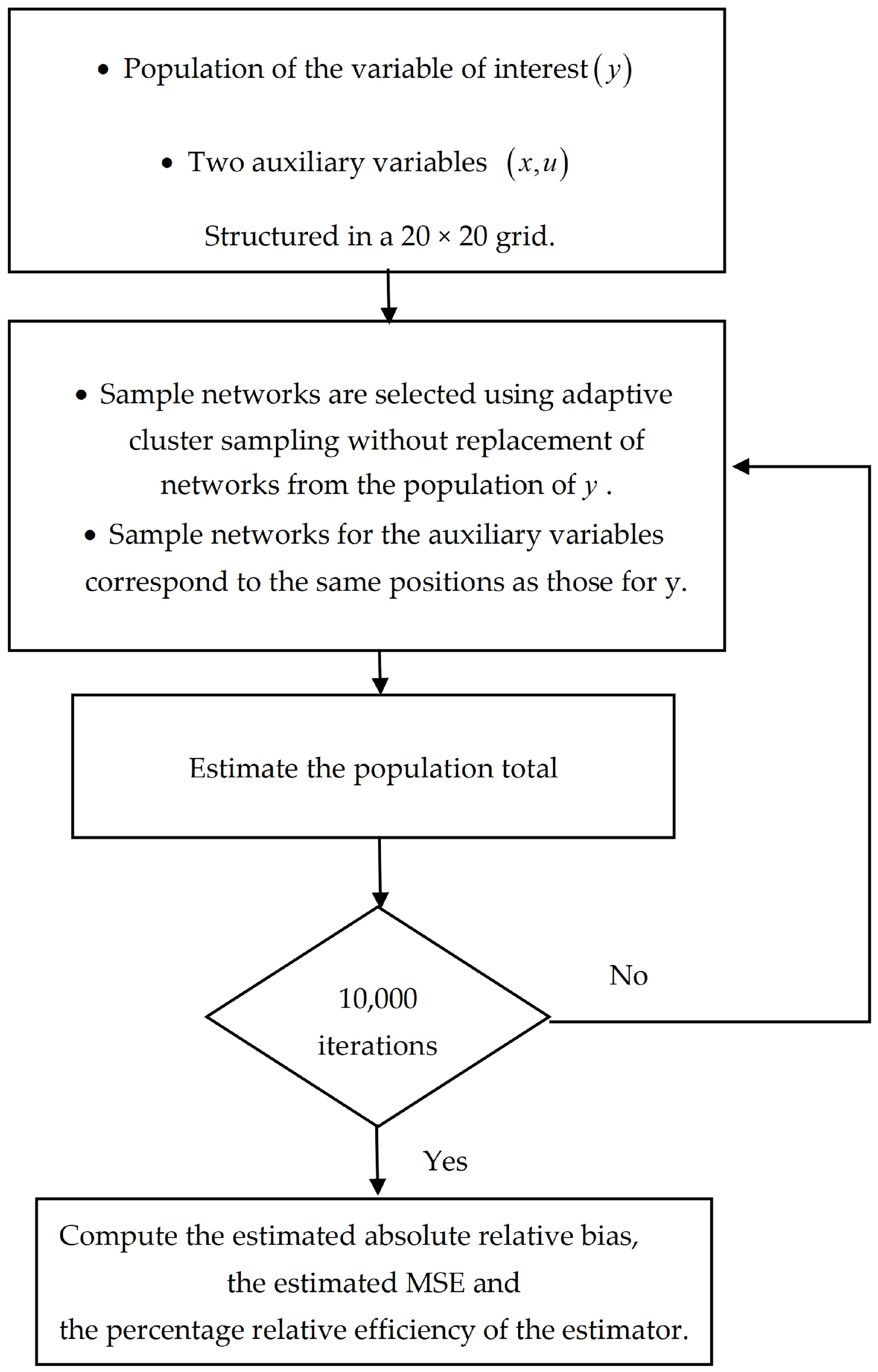
5.1. Simulation Study

The population of the variable of interest and the two auxiliary variables was based on the study by Nipaporn and Kumphon [15], consisting of a population size of 20 rows and 20 columns, or 400 units (Figure A1, Figure A2 and Figure A3). The parameter values were ${\tau }_y=489$, ${\tau }_x=222$, ${\tau }_u=1008$, ${\rho }_{yx}=0.91$, and ${\rho }_{yu}=0.87$. For each iteration, the initial sample units were selected by simple random sampling. The condition for adding sample units was defined by $C=\{y:y>0\}$. A total of 10,000 iterations were performed for each estimator. The number of networks were varied as n = 2, 5, 10, 15, 20, 25, and 50.

The estimated absolute relative bias was defined as

$$RB\left({\widehat{\tau }}_y\right)={\displaystyle \frac{1}{\mathrm{10,000}}}\sum _{i=1}^{\mathrm{10,000}}{\displaystyle \frac{\left|{\left({\widehat{\tau }}_y\right)}_i-{\tau }_y\right|}{{\tau }_y}}.$$

The estimated MSE of the estimator was defined as

$$MSE\left({\widehat{\tau }}_y\right)={\displaystyle \frac{1}{\mathrm{10,000}}}\sum _{i=1}^{\mathrm{10,000}}{\left({\left({\widehat{\tau }}_y\right)}_i-{\tau }_y\right)}^2.$$

The percentage relative efficiency of the proposed estimator was compared with ${\left({\widehat{\tau }}_y\right)}_{Raj}$ was defined as

$$PRE{\left({\widehat{\tau }}_y\right)}_{pro}={\displaystyle \frac{MSE{\left({\widehat{\tau }}_y\right)}_{Raj}}{MSE{\left({\widehat{\tau }}_y\right)}_{pro}}}\times 100.$$

The estimated absolute relative bias, estimated mean square error (MSE), and percentage relative efficiency of the estimators using two auxiliary variables under adaptive cluster sampling with networks selected without replacement were calculated. Figure 2 presents a flowchart outlining the steps of the simulation study, and the results are presented in

Table 1. The estimated absolute relative bias of the estimators for the total population of the variable of interest.

n	$\mathit{RB}{\left({\widehat{\mathit{\tau }}}_{\mathit{y}}\right)}_{\mathit{pro}}$
	${\mathit{T}}_{\mathit{1}}={\mathit{T}}_{\mathit{2}}=\mathit{1}$	${\mathit{T}}_{\mathit{1}}={\mathit{T}}_{\mathit{2}}=-\mathit{1}$	$$\begin{gathered} {\mathit{T}}_{\mathit{1}}=-\mathit{1} \\ {\mathit{T}}_{\mathit{2}}=\mathit{1} \end{gathered}$$	$$\begin{gathered} {\mathit{T}}_{\mathit{1}}={\mathit{T}}_{\mathit{1}}^{\ast } \\ {\mathit{T}}_{\mathit{2}}={\mathit{T}}_{\mathit{2}}^{\ast } \end{gathered}$$
2	0.9091	43.7092	0.0409	0.7103
5	0.5723	9.6476	0.0272	0.4120
10	0.4252	3.9173	0.0215	0.1237
15	0.3712	2.0932	0.0141	0.1210
20	0.3167	1.2775	0.0088	0.0960
25	0.3134	1.1377	0.0082	0.0765
50	0.1912	0.4281	0.0025	0.0143

$Note$: $T_1^{\ast }$ and $T_2^{\ast }$ are the optimum values of $T_1$ and $T_2$, respectively.

,

Table 2. The estimated MSE of the estimators for the total population of the variable of interest.

n	$\mathit{E}\left(\mathit{\nu }\right)$	$\mathit{MSE}{\left({\widehat{\mathit{\tau }}}_{\mathit{y}}\right)}_{\mathit{Raj}}$	$\mathit{MSE}{\left({\widehat{\mathit{\tau }}}_{\mathit{y}}\right)}_{\mathit{pro}}$
			${\mathit{T}}_{\mathit{1}}={\mathit{T}}_{\mathit{2}}=\mathit{1}$	${\mathit{T}}_{\mathit{1}}={\mathit{T}}_{\mathit{2}}=-\mathit{1}$	${\mathit{T}}_{\mathit{1}}=\mathit{1}$, ${\mathit{T}}_{\mathit{2}}=-\mathit{1}$	${\mathit{T}}_{\mathit{1}}=-\mathit{1}$, ${\mathit{T}}_{\mathit{2}}=\mathit{1}$	${\mathit{T}}_{\mathit{1}}={\mathit{T}}_{\mathit{1}}^{\ast },{\mathit{T}}_{\mathit{2}}={\mathit{T}}_{\mathit{2}}^{\ast }$
2	6.8466	968,885.0341	204,764.3145	26,322,915,632.8267	926,194.3208	1,445,829.5306	188,667.2977
5	16.1432	375,678.8942	132,903.3653	556,216,006.2863	375,147.0977	535,979.9843	121,855.7443
10	29.3040	185,513.8035	146,738.8306	68,892,932.1431	172,073.9448	291,531.9326	68,099.7147
15	39.5225	117,455.5717	245,276.4686	16,271,424.1794	111,666.6914	176,639.4646	45,295.0030
20	53.0735	80,580.0398	309,571.7174	4,919,034.4968	76,522.4944	116,484.1294	27,811.8563
25	59.9526	64,537.0999	272,468.2427	3,344,904.9521	59,331.5526	100,902.1119	23,029.4124
50	93.7806	25,465.4180	84,934.4510	630,026.2443	22,545.9512	41,470.0784	5722.4797

$Note$: $T_1^{\ast }$ and $T_2^{\ast }$ are the optimum values of $T_1$ and $T_2$, respectively.

and

Table 3. The percentage relative efficiency of the estimators for the total population of the variable of interest.

n	$\mathit{PRE}{\left({\widehat{\mathit{\tau }}}_{\mathit{y}}\right)}_{\mathit{Raj}}$	$\mathit{PRE}{\left({\widehat{\mathit{\tau }}}_{\mathit{y}}\right)}_{\mathit{pro}}$
		${\mathit{T}}_{\mathit{1}}={\mathit{T}}_{\mathit{2}}=\mathit{1}$	${\mathit{T}}_{\mathit{1}}={\mathit{T}}_{\mathit{2}}=-\mathit{1}$	${\mathit{T}}_{\mathit{1}}=\mathit{1}$, ${\mathit{T}}_{\mathit{2}}=-\mathit{1}$	${\mathit{T}}_{\mathit{1}}=-\mathit{1}$, ${\mathit{T}}_{\mathit{2}}=\mathit{1}$	${\mathit{T}}_{\mathit{1}}={\mathit{T}}_{\mathit{1}}^{\ast },{\mathit{T}}_{\mathit{2}}={\mathit{T}}_{\mathit{2}}^{\ast }$
2	100	473.1708	0.0037	104.6093	67.0124	513.5416
5	100	282.6707	0.0675	100.1418	70.0920	308.2981
10	100	126.4245	0.2693	107.8105	63.6341	272.4149
15	100	47.8870	0.7219	105.1841	66.4945	259.3124
20	100	26.0295	1.6381	105.3024	69.1768	289.7327
25	100	23.6861	1.9294	108.7737	63.9601	280.2377
50	100	29.9824	4.0420	112.9490	61.4067	445.0067

$Note$: $T_1^{\ast }$ and $T_2^{\ast }$ are the optimum values of $T_1$ and $T_2$, respectively.

.

5.2. Discussion

The data revealed that the variable of interest was positively correlated with both auxiliary variables. However, the correlation between the variable of interest and auxiliary variable x was stronger than its correlation with auxiliary variable u.

Our findings are summarized as follows:

• The results in Table 1 demonstrate that, for all estimators, the estimated absolute relative bias decreased as the network sample size increased. Among the estimators, the product-type estimator $\left(T_1=T_2=-1\right)$ consistently exhibited higher estimated absolute relative bias than the other estimators.
• Table 2 presents the estimated mean square error (MSE) of the estimators. Here, $MSE{\left({\widehat{\tau }}_y\right)}_{Raj}$ represents the estimated mean square error of the modified Des Raj estimator, which did not rely on auxiliary variable information, while $MSE{\left({\widehat{\tau }}_y\right)}_{pro}$ refers to the proposed estimator that incorporates two auxiliary variables. For all network sample sizes, the estimated mean square error of the proposed estimator ${\left({\widehat{\tau }}_y\right)}_{pro}$ was lower than that of the modified Des Raj estimator, ${\left({\widehat{\tau }}_y\right)}_{Raj}$, when $T_1=1$, $T_2=-1$ (ratio-cum-product-type estimator), and $T_1=T_1^{\ast }$, $T_2=T_2^{\ast }$ (the proposed estimator with optimal values). The proposed estimator ${\left({\widehat{\tau }}_y\right)}_{pro}$ with the optimal values as $T_1=T_1^{\ast }$, $T_2=T_2^{\ast }$ achieved the lowest estimated MSE compared to the settings $(T_1,T_2)=(1,1),(-1,-1),(1,-1)$, and $(-1,1)$, corresponding to ratio-type, product-type, ratio-cum-product type, and product-cum-ratio-type estimators, respectively. The estimated MSE of the product-type estimator was particularly high, as this estimator was applied in scenarios where the variable of interest and the auxiliary variables were related in opposing directions.
• Table 3 presents the percentage relative efficiency (PRE) of the proposed estimator compared to the modified Des Raj estimator ${\left({\widehat{\tau }}_y\right)}_{Raj}$, where $PRE{\left({\widehat{\tau }}_y\right)}_{Raj}$ is set to 100. A PRE value greater than 100 indicates that the estimator is more efficient than ${\left({\widehat{\tau }}_y\right)}_{Raj}$. The results show that the product-type and product-cum-ratio-type estimators exhibited lower efficiency than ${\left({\widehat{\tau }}_y\right)}_{Raj}$ across all network sample sizes. The ratio-type estimator demonstrated higher efficiency than ${\left({\widehat{\tau }}_y\right)}_{Raj}$ when the network sample size was small. Meanwhile, the ratio-cum-product-type estimator and the proposed estimator with optimal values of $T_1$ and $T_2$ as $T_1=T_1^{\ast },T_2=T_2^{\ast }$ had higher efficiency than ${\left({\widehat{\tau }}_y\right)}_{Raj}$ for all network sample sizes. Among all the estimators, the proposed estimator with optimal values of $T_1$ and $T_2$ was the most efficient.

6. Conclusions

In adaptive cluster sampling, the initial units are selected using simple random sampling without replacement, but networks can be selected more than once. Salehi and Seber [12] proposed an adaptive cluster sampling with networks selected without replacement by introducing an estimator based on the Des Raj estimator, ${\left({\widehat{\tau }}_y\right)}_{\mathrm{Raj}}$. In some situations, auxiliary information related to the variable of interest is utilized to improve the precision of the estimator. Chutiman and Chiangpradit [22] proposed a ratio estimator that uses a single auxiliary variable in adaptive cluster sampling with networks selected without replacement. This study presented a multiplicative generalization of the estimator, incorporating two auxiliary variables as

$${\left({\widehat{\tau }}_y\right)}_{pro}={\left({\widehat{\tau }}_y\right)}_{Raj}{\left[{\displaystyle \frac{{\tau }_x}{{\left({\widehat{\tau }}_x\right)}_{Raj}}}\right]}^{T_1}{\left[{\displaystyle \frac{{\tau }_u}{{\left({\widehat{\tau }}_u\right)}_{Raj}}}\right]}^{T_2}.$$

The bias and mean square error (MSE) of the proposed estimator were derived, and the optimum values of $T_1$ and $T_2$ were determined by minimizing their MSE. When inappropriate values of $T_1$ and $T_2$ were used, the proposed estimator was less efficient than the modified Des Raj estimator ${\left({\widehat{\tau }}_y\right)}_{Raj}$, which does not rely on auxiliary variable information. However, the optimal values of $T_1$ and $T_2$ yielded the lowest MSE of the estimator. The performance of the proposed estimator was further validated through numerical simulations. Table 2 and Table 3 reveal that while the variable of interest was positively correlated with the two auxiliary variables, the ratio-type estimator did not outperform the modified Des Raj estimator at any network sample size. Conversely, the proposed estimator was the most efficient when $T_1$ and $T_2$ were set to their optimal values, i.e., $T_1=T_1^{\ast }$ and $T_2=T_2^{\ast }$. Comprehensive analysis and the interpretation of the results demonstrate that the proposed estimator with optimum values of $T_1$ and $T_2$ achieved superior performance metrics in terms of both MSE and percentage relative efficiency. These findings highlight its enhanced accuracy compared to the alternative estimators examined. Future research should focus on assessing the robustness of the proposed estimator under different population structures and varying degrees of spatial clustering. Additionally, further studies should explore the integration of more than two auxiliary variables to enhance estimation efficiency in adaptive cluster sampling without the replacement of networks.

References

1. Thompson, S.K. Adaptive cluster sampling. J. Am. Statist. Assoc. 1990, 85, 1050–1059. [Google Scholar] [CrossRef]
2. Magnussen, S.; Kurz, W.; Leckie, D.G.; Paradine, D. Adaptive cluster sampling for estimation of deforestation rates. Eur. J. For. Res. 2005, 124, 207–220. [Google Scholar] [CrossRef]
3. Noon, B.R.; Ishwar, N.M.; Vasudevan, K. Efficiency of adaptive cluster and random sampling in detecting terrestrial herpetofauna in a tropical rainforest. Wildl. Soc. Bull. 2006, 34, 59–68. [Google Scholar] [CrossRef]
4. Sullivan, W.P.; Morrison, B.J.; Beamish, F.W.H. Adaptive cluster sampling: Estimating density of spatially autocorrelated larvae of the sea lamprey with improved precision. J. Great Lakes Res. 2008, 34, 86–97. [Google Scholar] [CrossRef]
5. Smith, D.R.; Villella, R.F.; Lemarié, D.P. Application of adaptive cluster sampling to low-density populations of freshwater mussels. Environ. Ecol. Stat. 2003, 10, 7–15. [Google Scholar] [CrossRef]
6. Conners, M.E.; Schwager, S.J. The use of adaptive cluster sampling for hydroacoustic surveys. ICES J. Mar. Sci. 2002, 59, 1314–1325. [Google Scholar] [CrossRef]
7. Olayiwola, O.M.; Ajayi, A.O.; Onifade, O.C.; Wale-Orojo, O.; Ajibade, B. Adaptive cluster sampling with model based approach for estimating total number of Hidden COVID-19 carriers in Nigeria. Stat. J. IAOS 2020, 36, 103–109. [Google Scholar] [CrossRef]
8. Chandra, G.; Tiwari, N.; Nautiyal, R. Adaptive cluster sampling-based design for estimating COVID-19 cases with random samples. Curr. Sci. 2021, 120, 1204–1210. [Google Scholar] [CrossRef]
9. Stehlík, M.; Kiseľák, J.; Dinamarca, A.; Alvarado, E.; Plaza, F.; Medina, F.A.; Stehlíková, S.; Marek, J.; Venegas, B.; Gajdoš, A.; et al. REDACS: Regional emergency-driven adaptive cluster sampling for effective COVID-19 management. Stoch. Anal. Appl. 2022, 41, 474–508. [Google Scholar] [CrossRef]
10. Hwang, J.; Bose, N.; Fan, S. AUV adaptive sampling methods: A Review. Appl. Sci. 2019, 9, 3145. [Google Scholar] [CrossRef]
11. Giouroukis, D.; Dadiani, A.; Traub, J.; Zeuch, S.; Markl, V. A survey of adaptive sampling and filtering algorithms for the internet of things. In Proceedings of the 14th ACM International Conference on Distributed and Event Based Systems, Montreal, QC, Canada, 13–17 July 2020; pp. 27–38. [Google Scholar] [CrossRef]
12. Salehi, M.M.; Seber, G.A.F. Adaptive cluster sampling with networks selected without replacement. Biometrika 1977, 84, 209–219. [Google Scholar] [CrossRef]
13. Chao, C.T. Ratio estimation on adaptive cluster sampling. J. Chin. Stat. Assoc. 2004, 42, 307–327. [Google Scholar] [CrossRef]
14. Dryver, A.L.; Chao, C.T. Ratio estimators in adaptive cluster sampling. Environmetric 2007, 18, 607–620. [Google Scholar] [CrossRef]
15. Chutiman, N.; Kumphon, B. Ratio estimator using two auxiliary variables for adaptive cluster sampling. Thail. Stat. 2008, 6, 241–256. [Google Scholar]
16. Chutiman, N. Adaptive cluster sampling using auxiliary variable. J. Math. Stat. 2013, 9, 249–255. [Google Scholar] [CrossRef]
17. Yadav, S.K.; Misra, S.; Mishra, S. Efficient estimator for population variance using auxiliary variable. Am. J. Oper. Res. 2016, 6, 9–15. [Google Scholar] [CrossRef]
18. Chaudhry, M.S.; Hanif, M. Generalized exponential-cum-exponential estimator in adaptive cluster sampling. Pak. J. Stat. Oper. Res. 2015, 11, 553–574. [Google Scholar] [CrossRef]
19. Singh, R.; Mishra, R. Transformed ratio type estimators under adaptive cluster sampling an application to covid-19. J. Stat. Appl. Probab. Lett. 2022, 9, 63–70. [Google Scholar] [CrossRef]
20. Bhat, A.A.; Sharma, M.; Shah, M.; Bhat, M. Generalized ratio type estimator under adaptive cluster sampling. J. Sci. Res. 2022, 67, 46–51. [Google Scholar] [CrossRef]
21. Mishra, R.; Singh, R.; Raghav, Y.S. On combining ratio and product type estimators for estimation of finite population mean in adaptive cluster sampling design. Braz. J. Biom. 2024, 42, 412–420. [Google Scholar] [CrossRef]
22. Chutiman, N.; Chiangpradit, M. Ratio estimator in adaptive cluster sampling without replacement of networks. J. Probab. Stat. 2014, 2014, 726398. [Google Scholar] [CrossRef]
23. Raj, D. Some Estimators in sampling with varying probabilities without replacement. J. Am. Stat. Assoc. 1956, 51, 269–284. [Google Scholar] [CrossRef]
24. Gupta, S.; Shabbir, J. On the use of transformed auxiliary variables in estimating population mean by using two auxiliary variables. J. Stat. Plan. Inference 2007, 137, 1606–1611. [Google Scholar] [CrossRef]
Figure 1. Example of a network (shaded in green), where the unit marked with an asterisk represents the initial sampling unit.
Symmetry 17 00375 g001
Figure 2. The steps of the simulation study for each sample size of networks.
Symmetry 17 00375 g002