About a Classical Gravitational Interaction in a General Non-Inertial Reference Frame: Applications on Celestial Mechanics and Astrodynamics

Abstract

This paper offers new insights into gravitational interactions within a general non-inertial reference frame. By utilizing symbolic tensor calculus, the study establishes a unified framework that connects time derivatives in non-inertial frames to those in inertial frames. The research introduces new first integrals of motion for a system of many particles in arbitrary non-inertial and barycentric rotating reference frames. These first integrals provide a kinematic and geometric visualization of motion in non-inertial frames. Additionally, a generalized potential energy function is presented for broader applicability. For the gravitational two-body problem, the paper delivers a closed-form, coordinate-free solution for the motion of each body relative to the original frame. Consequently, sufficient conditions for stability against collisions are established within the context of the two-body problem in a non-inertial reference frame. Furthermore, the paper examines the relative orbital motion of spacecraft, presenting a closed-form and coordinate-free solution in the local vertical local horizontal (LVLH) non-inertial frame, which is centered on the center of mass of the main spacecraft.

1. Introduction

The N-body problem is a fundamental mathematical model with significant applications in astrophysics and astrodynamics. It plays a crucial role in understanding the motion of celestial bodies such as the moon, planets, asteroids, comets, and stars across various systems, ranging from binary stars to galaxies [1,2,3,4,5,6,7,8,9,10,11,12,13,14,15,16,17,18,19,20,21,22]. In the inertial case, the equations can be solved analytically for N = 1 and N = 2. However, for N $\ge$ 3, the problem becomes much more complex, particularly in the general three-body problem, which is one of the richest unsolved dynamical problems [2,3,7,17,18,19,20,21,22,23,24,25,26,27,28,29,30,31,32]. For scenarios dominated by a massive body, approximate methods based on perturbation expansions have been developed, especially in many planetary contexts. The many-body problem’s unique properties and inherent complexities have captured the attention of mathematicians throughout history [1,2,3,4,5,6,7,8,9,10,11,12,13,14,15,16,17,18,19,20,21,22,23,24,25,26,27,28,29,30,31,32]. Since no general solution is known, researchers continue to search for unique solutions, including periodic and escape solutions [9,10,11,12,13,14,15,16,17,18,19,20,21,22,23]. This paper presents the results concerning the N-body problem in a general non-inertial reference frame. When studying the equations of motion in a non-inertial reference frame, it is essential to consider the effects of Coriolis, Euler, centrifugal, and translational inertial forces. This inclusion significantly complicates the mathematical modeling of the system of many bodies. In this context, the paper extends the concepts of linear momentum, angular momentum, and system energy to allow the definition of first integrals as in inertial cases. The approach to motion in non-inertial reference systems is fundamentally symbolic. In the first step, the problem is resolved within a non-rotating frame. The non-inertial frame of reference is then “frozen” at the initial time. In the second step, the solution to the non-inertial problem is derived by applying a specific tensor to the solution obtained in the previous step. This process relies on symbolic calculus involving proper orthogonal tensors and skew-symmetric tensor-valued functions, which are connected through the Poisson–Darboux equation and a differentiation operator. The relationship between the derivative in a non-inertial frame and that in an inertial frame is presented. This paper also demonstrates a new first integral of N-body motion within any arbitrary non-inertial frame in relation to a barycenter in a rotating reference frame. To the best of the author’s knowledge, these results are original and presented here for the first time. The new first integrals provide a kinematic and geometrical visualization of motion in the non-inertial reference frame, and a generalized potential energy function is introduced in a broader context. For the two-body problem, a closed-form coordinate-free solution for the motion of each body concerning the original frame is provided. Consequently, sufficient conditions for stability against impact in the two-body problem are also identified. The problem of relative orbital motion of spacecraft is solved in a closed and coordinate-free form.

The structure of the paper is as follows: In Section 2, the connection between derivatives in non-inertial and inertial frames is established using the appropriate orthogonal proper Euclidean tensor and skew-symmetric tensor related through the Poisson–Darboux equation and a new differentiation operator. In Section 3 and Section 4, new first integrals for the N-body problem in arbitrary non-inertial frames are derived, with a specific focus on the barycenter rotating reference frame, which illustrates new first integrals. In Section 5, for the two-body problem, the closed-form coordinate-free solution for the law of motion of each body concerning the original frame is introduced. Firstly, the first integral of the dynamical system and the relative movements of the two particles in relation to a reference frame attached to the barycenter are presented, complete with closed-form equations of motion and novel features. This paper offers for the first time a comprehensive approach to the gravitational two-body problem in a general non-inertial reference frame. Furthermore, the paper examines the relative orbital motion of spacecraft, presenting a closed-form and coordinate-free solution in the local vertical local horizontal (LVLH) non-inertial frame, which is centered on the center of mass of the main spacecraft. Section 6 presents the conclusion, which discusses results and future work. Lastly, Appendix A includes the Poisson–Darboux kinematic equation, specifically demonstrated for closed-form solutions.

2. Mathematical Preliminaries

The present section is concerned with the key concepts associated with proper orthogonal tensorial maps, and their specific applications to understanding motion in systems with gravitational interactions, particularly in an arbitrary non-inertial reference frame. These maps are closely related to skew–symmetric tensorial maps corresponding to the instantaneous angular velocity of the non-inertial frame, and this relationship is described by the Poisson–Darboux kinematic equation. The results presented here were first discussed in references [33,34,35,36]. In the subsequent section, the utilization of orthogonal tensorial maps is employed for the purpose of analyzing motion in non-inertial reference frames.

2.1. A Tensor Operator

Rigid body rotation with arbitrary instantaneous angular velocity $\mathsf{\omega }$ is related to proper orthogonal tensor maps of real variable by a differential tensorial equation, like the one from attitude kinematics, which is also referred to as the Poisson–Darboux equation [35,36]:

Lemma 1.

[33] Consider the initial value tensor problem for any continuous $\tilde{\mathsf{\omega }}\in \mathit{s}{\mathit{o}}_3^{\mathbb{R}}$:

$$\dot{\mathbf{Q}}=\mathbf{Q}\tilde{\mathsf{\omega }}; \mathbf{Q}\left(t_0\right)={\mathbf{I}}_3,\hspace{1em}\forall \left(t_0\right)\ge 0.$$

(1)

 Then there exists a unique solution $\mathbf{Q}\in \mathbf{S}{\mathbf{O}}_3^{\mathbb{R}}$.

Proof .

See Appendix A. □

The unique solution to Equation (1) will be denoted ${\mathbf{F}}_{\mathsf{\omega }}$. The following lemma presents the properties of this proper orthogonal Euclidean tensorial map.

Lemma 2.

[33] The map ${\mathbf{F}}_{\mathsf{\omega }}$ satisfies the following properties:

1. 

${\mathbf{F}}_{\mathsf{\omega }}$ is invertible,

2. 

${\mathbf{F}}_{\mathsf{\omega }}\mathbf{u}\cdot {\mathbf{F}}_{\mathsf{\omega }}\mathbf{u}=\mathbf{u}\cdot \mathbf{v},\forall \mathbf{u},\mathbf{v}\in {\mathbf{V}}_3^{\mathbb{R}}$;

3. 

$‖{\mathbf{F}}_{\mathsf{\omega }}\mathbf{u}‖=‖\mathit{u}‖,\forall \mathbf{u}\in {\mathbf{V}}_3^{\mathbb{R}}$;

4. 

${\mathbf{F}}_{\mathsf{\omega }}\left(\mathbf{u}\times \mathbf{v}\right)={\mathbf{F}}_{\mathsf{\omega }}\mathbf{u}\times {\mathbf{F}}_{\mathsf{\omega }}\mathbf{v},\forall \mathbf{u},\mathbf{v}\in {\mathbf{V}}_3^{\mathbb{R}}$;

5. 

${\displaystyle \frac{d}{dt}}{\mathbf{F}}_{\mathsf{\omega }}\mathbf{u}={\mathbf{F}}_{\mathsf{\omega }}\left(\dot{\mathbf{u}}+\mathsf{\omega }\times \mathbf{u}\right),\forall \mathbf{u}\in {\mathbf{V}}_3^{\mathbb{R}}$, differentiable.

6. 

${\displaystyle \frac{d^2}{ d{t}^2}}{\mathbf{F}}_{\mathsf{\omega }}\mathbf{u}={\mathbf{F}}_{\mathsf{\omega }}\left(\ddot{\mathbf{u}}+2\mathsf{\omega }\times \dot{\mathbf{u}}+\mathsf{\omega }\times \left(\mathsf{\omega }\times \mathbf{u}\right)+\dot{\mathsf{\omega }}\times \mathbf{u}\right),\forall \mathbf{u}\in {\mathbf{V}}_3^{\mathbb{R}}$, differentiable.

The proof of Lemma 2 may be performed by elementary manipulations; therefore, it is omitted.

2.2. Comments and Remarks

The following denotation is introduced:

$${\left({\mathbf{F}}_{\mathsf{\omega }}\right)}^{-1}\triangleq {\mathbf{R}}_{-\mathsf{\omega }},$$

(2)

It follows that ${\mathbf{R}}_{-\mathsf{\omega }}$ is the proper orthogonal Euclidean tensor map associated to the instantaneous angular velocity $-\mathsf{\omega }$. Therefore, the following is a unique solution to the IVP:

$${\dot{\mathbf{R}}}_{-\mathsf{\omega }}+\tilde{\mathsf{\omega }}{\mathbf{R}}_{-\mathsf{\omega }}=0; {\mathbf{R}}_{-\mathsf{\omega }}\left(t_0\right)={\mathbf{I}}_3,$$

(3)

2.3. A Vector Differentiation Operator

We introduce a differential operator related to the angular velocity $\mathsf{\omega }$ of the reference frame with which an arbitrary vector is associated. It is a derivation-like operator, and its use will be revealed further. Define the vector valued function differentiation rule ${(\hspace{1em})}^{\prime }:{\mathbf{V}}_3^{\mathbb{R}}\to {\mathbf{V}}_3^{\mathbb{R}}$ thus:

$${(\hspace{1em})}^{\prime }=\stackrel{.}{\left((\hspace{1em})\right)}+\mathsf{\omega }\times (\hspace{1em}).$$

(4)

For a differentiable vectorial map $\mathbf{u}:\mathbb{R}\to {\mathbf{V}}_3^{\mathbb{R}}$, the following stands:

$$\mathbf{u}\prime =\dot{\mathbf{u}}+\mathsf{\omega }\times \mathbf{u}.$$

(5)

The next results present the properties of this operator together with the link to the previously defined tensor valued function ${\mathbf{F}}_{\mathsf{\omega }}$.

Lemma 3

([33]). The following affirmations hold:

1. 

${\mathsf{\omega }}^{\prime }=\dot{\mathsf{\omega }}$;

2. 

$\left(\mathbf{u}+\mathbf{v}\right)\prime =\mathbf{u}\prime +\mathbf{v}\prime ,\left(\forall \right)\mathbf{u},\mathbf{v}\in C^2\left({\mathrm{V}}_3^{\mathbb{R}}\right)$  ;

3. 

${\left(\lambda \mathbf{u}\right)}^{\prime }=\dot{\lambda }\mathbf{u}+\mathsf{\lambda }{\mathbf{u}}^{\prime },\left(\forall \right)\mathbf{u}\in C^2\left({\mathrm{V}}_3^{\mathbb{R}}\right),\left(\forall \right)\lambda :\mathbb{R}\to \mathbb{R}$  , differentiable.

4. 

${\left(\mathbf{u}\times \mathbf{v}\right)}^{\prime }={\mathbf{u}}^{\prime }\times \mathbf{v}+\mathbf{u}\times {\mathbf{v}}^{\prime },\left(\forall \right)\mathbf{u},\mathbf{v}\in C^2\left({\mathrm{V}}_3^{\mathbb{R}}\right)$;

5. 

${\mathbf{u}}^{\prime }\cdot \mathbf{v}+\mathbf{u}\cdot {\mathbf{v}}^{\prime }=\dot{\mathbf{u}}\cdot \mathbf{v}+\mathbf{u}\cdot \dot{\mathbf{v}}={\displaystyle \frac{d}{dt}}\left(\mathbf{u}\cdot \mathbf{v}\right),\left(\forall \right)\mathbf{u},\mathbf{v}\in C^2\left({\mathrm{V}}_3^{\mathbb{R}}\right)$;

6. 

$\mathbf{u}″=\ddot{\mathbf{u}}+2\mathsf{\omega }\times \dot{\mathbf{u}}+\mathsf{\omega }\times \left(\mathsf{\omega }\times \mathbf{u}\right)+\dot{\mathsf{\omega }}\times \mathbf{u},\left(\forall \right)\mathbf{u}\in C^2\left({\mathrm{V}}_3^{\mathbb{R}}\right)$;

7. 

${\displaystyle \frac{d}{dt}}\left({\mathbf{F}}_{\mathsf{\omega }}\mathbf{u}\right)={\mathbf{F}}_{\mathsf{\omega }}\left(\mathbf{u}\prime \right),\left(\forall \right)\mathbf{u}\in C^2\left({\mathrm{V}}_3^{\mathbb{R}}\right)$;

8. 

${\displaystyle \frac{d^2}{{dt}^2}}\left({\mathbf{F}}_{\mathsf{\omega }}\mathbf{u}\right)={\mathbf{F}}_{\mathsf{\omega }}\left(\mathbf{u}″\right),\left(\forall \right)\mathbf{u}\in C^2\left({\mathrm{V}}_3^{\mathbb{R}}\right)$;

9. 

${\left.{\mathbf{F}}_{\mathsf{\omega }}\mathbf{u}\right|}_{t=t_0}=\mathbf{u}\left(t_0\right); {\displaystyle \frac{d}{dt}}{\left.\left({\mathbf{F}}_{\mathsf{\omega }}\mathbf{u}\right)\right|}_{t=t_0}=\dot{\mathbf{u}}\left(t_0\right)+\mathsf{\omega }\left(t_0\right)\times \mathbf{u}\left(t_0\right).$

Elementary mathematical manipulations may prove Lemma 3; therefore, it will not be presented here.

The vector differentiation defined in Equation (4) makes the connection between the time derivative of a vector referred to as a reference frame that rotates with instantaneous angular velocity $\mathsf{\omega }$ (denoted with a dot above) and the time derivative of the same vector referred to as an inertial reference frame (denoted with prime).

The anti-derivation rule associated to the differentiation rule $\left( \right)\prime$ is presented below.

Lemma 4

([33]). Consider $\mathit{v}=\mathit{v}\left(t\right)$ a continuous vector valued function. The solution to the IVP 

$${\mathbf{r}}^{\prime }=\mathbf{v},\mathbf{r}\left(t_0\right)={\mathbf{r}}_0$$

(6)

is expressed thus:

$$\mathbf{r}={\mathbf{R}}_{-\mathsf{\omega }}\left[{\mathbf{r}}_0+\underset{t_0}{\overset{t}{\int }}{\mathbf{R}}_{-\mathsf{\omega }}^T\left(s\right)\mathbf{v}\left(s\right)ds\right]$$

(7)

where ${\mathbf{R}}_{-\mathsf{\omega }}$ is defined in Equation (3).

Proof. 

Applying the tensor operator ${\mathbf{F}}_{\mathsf{\omega }}$ to the IVP (6) and using point (8), and point (7) of Lemma 3 together with the initial conditions from Equation (6), it follows that

$${\displaystyle \frac{d}{dt}}\left({\mathbf{F}}_{\mathsf{\omega }}\mathbf{r}\right)={\mathbf{F}}_{\mathsf{\omega }}\mathbf{v}; {\left.\left({\mathbf{F}}_{\mathsf{\omega }}\mathbf{r}\right)\right|}_{t=t_0}={\mathbf{r}}_0.$$

(8)

The first-order differential equation is as follows:

$${\mathbf{F}}_{\mathsf{\omega }}\mathbf{r}={\mathbf{r}}_0+\underset{t_0}{\overset{t}{\int }}{\mathbf{R}}_{-\mathsf{\omega }}^T\left(s\right)\mathbf{v}\left(s\right)ds$$

(9)

Equation (7) is obtained by applying the tensor ${\mathbf{R}}_{-\mathsf{\omega }}$ to the equality (9). The proof is finalized. □

Remark 1.

From Lemma 4, it follows that if a vector map $\mathit{r}:{\mathbb{R}}_{+}\to {\mathit{V}}_3^{\mathbb{R}}$ satisfies the initial value problem below,

$$\mathbf{r}\prime =\mathbf{0},\mathbf{r}\left(t_0\right)={\mathbf{r}}_0$$

(10)

then vector $\mathbf{r}$is the rotation with angular velocity $-\mathsf{\omega }$ of a constant vector ${\mathbf{r}}_0=\mathbf{r}\left(t_0\right)$:

$$\mathbf{r}={\mathbf{R}}_{-\mathsf{\omega }}{\mathbf{r}}_0$$

(11)

This remark will make it possible to offer a geometric interpretation of the first integrals of the N-body dynamical system.

Lemma 5.

The solution to the IVP is thus:

$$\left\{\begin{array}{l}\ddot{\mathbf{r}}+2\mathsf{\omega }\times \dot{\mathbf{r}}+\mathsf{\omega }\times \left(\mathsf{\omega }\times \mathbf{r}\right)+\dot{\mathsf{\omega }}\times \mathbf{r}=f\left(\mathrm{r}\right)\widehat{\mathbf{r}},\\ \left\{\begin{array}{l}\mathbf{r}\left(t_0\right)={\mathbf{r}}^0\\ \dot{\mathbf{r}}\left(t_0\right)={\mathbf{v}}^0\end{array}\right.\end{array}\right.$$

(12)

where $\mathsf{\omega }$  is a differentiable vector time function, $f=f\left(r\right)$ is a real continuum function by $\mathrm{r}=‖\mathbf{r}‖$, and $\widehat{\mathbf{r}}$ is unit vector of $\mathbf{r}$, is obtained by applying the tensor operator ${\mathbf{R}}_{-\mathsf{\omega }}$ to the solution of the IVP:

$$\left\{\begin{array}{l}\ddot{\mathbf{r}}=f\left(\mathrm{r}\right)\widehat{\mathbf{r}},\\ \left\{\begin{array}{l}\mathbf{r}\left(t_0\right)={\mathbf{r}}^0\\ \dot{\mathbf{r}}\left(t_0\right)={\mathbf{v}}^0+{\mathsf{\omega }}^0\times {\mathbf{r}}^0\end{array}\right.\end{array}\right.,$$

(13)

where ${\mathsf{\omega }}^0=\mathsf{\omega }\left({\mathrm{t}}_0\right).$

Proof. 

Equation (13) may be written using the previous considerations:

$$\mathbf{r}\prime \prime =f\left(\mathrm{r}\right)\widehat{\mathbf{r}}.$$

(14)

Apply the operator ${\mathbf{F}}_{\mathsf{\omega }}$ to Equation (14) and perform the change of variable $\mathbf{r}$ in ${\mathbf{F}}_{\mathsf{\omega }}$; the result is obtained from simple manipulations and Equation (2). □

IVP (12) is a motion problem in an isotropic central force field in rotating reference frame with instantaneous angular velocity $\mathsf{\omega }$. Previous results offer a simple way to solve this problem following these steps (also see Refs. [33,37]):

(1)

Solve IVP (12), the inertial problem in the frozen non-inertial reference frame at ${\mathrm{t}=\mathrm{t}}_0;$

(2)

Apply ${\mathbf{R}}_{-\mathsf{\omega }}$ to the solution to the IVP (12) to determine the solution to IVP (13).

3. The N-Body Problem in a Non-Inertial Reference Frame: Some First Integrals

This Section studies the global mechanical characteristics of the whole system of N-body particles. For values of N greater than two, the separation of the problem into single-particle problems is no longer possible. By introducing replicas for the classic kinetical global characteristics of a system of particles (linear momentum, angular momentum, kinetic energy), interesting first integrals are deduced.

When considering the effects of Coriolis inertial forces, Euler and centrifugal inertial forces, and translational inertial forces, the mathematical model for the N-body problem in non-inertial reference frames is represented by initial value problems:

$$\left\{\begin{array}{l}{m}_i{\ddot{\mathbf{r}}}_i+2m_i\mathsf{\omega }\times {\dot{\mathbf{r}}}_i+m_i\mathsf{\omega }\times \left(\mathsf{\omega }\times {\mathbf{r}}_i\right)+m_i\dot{\mathsf{\omega }}\times {\mathbf{r}}_i+m_i{\mathbf{a}}_{\mathcal{F}}={\mathbf{F}}_i,\\ \left\{\begin{array}{l}{\mathbf{r}}_i\left(t_0\right)={\mathbf{r}}_i^0\\ {\dot{\mathbf{r}}}_i\left(t_0\right)={\mathbf{v}}_i^0\end{array},\right.i=\overline{1,\mathrm{N}}\end{array}\right.$$

(15)

In Equation (15), ${\mathbf{r}}_i$ denotes the position vector; ${\dot{\mathbf{r}}}_i$ the velocity vector of the particle $P_i,i=\overline{1,\mathrm{N}}$, related to the non-inertial reference frame; $m_i$ is the masses of the particle of order $i=\overline{1,\mathrm{N}}$; ${\mathbf{a}}_{\mathcal{F}}$ is the acceleration of reference frame; and $\mathsf{\omega }$ is the instantaneous angular velocity of the non-inertial reference frame. The vector map of time variable $\mathsf{\omega }$ is supposed to be differentiable, and ${\mathbf{a}}_{\mathcal{F}}$ is supposed to be continuous.

In Equation (15), the vector ${\mathbf{F}}_i=\sum _j^n{\mathbf{F}}_{ij}$ denotes the force that acts upon the particle $P_i$ due to the interaction with particles $P_{j}i\ne j, i,j=\overline{1,\mathrm{N}}$. ${\mathbf{F}}_{ij}$ is the interacting force of particle $P_i$ due to the interaction with particle $P_{j}i\ne j$. The approach assumes ${\mathbf{F}}_{ij}$ an isotropic central function:

$${\mathbf{F}}_{ij}={\mathbf{F}}_{ij}\left(‖{\mathbf{r}}_j-{\mathbf{r}}_i‖\right),\hspace{1em}i\ne j,\hspace{1em}i,j=\overline{1,\mathrm{N}}.$$

(16)

From the principle of reciprocal interactions, it follows that

$$\left\{\begin{array}{l}{\mathbf{F}}_{ij}+{\mathbf{F}}_{ji}=\mathbf{0}; \\ {\mathbf{F}}_{ij}\times \left({\mathbf{r}}_j-{\mathbf{r}}_i\right)=\mathbf{0}.\end{array}\right.$$

(17)

$${\mathbf{F}}_{ij}=f\left({\mathrm{r}}_{ij}\right){\displaystyle \frac{{\mathbf{r}}_{ij}}{{\mathrm{r}}_{ij}}},$$

(18)

with continuous real valued function $f\left({\mathrm{r}}_{ij}\right)$ being prescribed by this denotation:

$${\mathbf{r}}_{ij}={\mathbf{r}}_j-{\mathbf{r}}_i$$

(19)

$${\mathrm{r}}_{ij}=‖{\mathbf{r}}_j-{\mathbf{r}}_i‖=‖{\mathbf{r}}_{ij}‖$$

(20)

In the case of gravitational interactions, (γ is a gravitational constant) let it be that

$$f\left({\mathrm{r}}_{ij}\right)=-\gamma {\displaystyle \frac{m_i·m_j}{{{\mathrm{r}}_{ij}}^2}},\hspace{1em}\hspace{1em}i\ne j,\hspace{1em}\hspace{1em}i,j=\overline{1,\mathrm{N}}$$

(21)

The Motion of the Barycenter of N-Body System

This section provides a closed-form solution for the motion of the barycenter of N-body system in an arbitrary non-inertial reference frame. First, let us denote the position vector:

$${\mathbf{r}}_C={\displaystyle \frac{\sum _{i=1}^N{m}_i{\mathbf{r}}_i}{\sum _{i=1}^N{m}_i}}.$$

(22)

Vector ${\mathbf{r}}_C$ models the position of the barycenter of the dynamical system comprising the N-body in relation to the non-inertial reference frame to which the motion is referred. The following statement holds:

$${\dot{\mathbf{r}}}_C={\displaystyle \frac{\sum _{i=1}^N{m}_i{\dot{\mathbf{r}}}_i}{\sum _{i=1}^N{m}_i}}.$$

(23)

By summarizing Equations (15) and (17) and considering Equations (22) and (23), we conclude that the vector function ${\mathbf{r}}_C$ satisfies the initial value problem presented below:

$$\left\{\begin{array}{l}{\ddot{\mathbf{r}}}_C+2\mathsf{\omega }\times {\dot{\mathbf{r}}}_C+\mathsf{\omega }\times \left(\mathsf{\omega }\times {\mathbf{r}}_C\right)+\dot{\mathsf{\omega }}\times {\mathbf{r}}_C+{\mathbf{a}}_{\mathcal{F}}=\mathbf{0},\\ \left\{\begin{array}{l}{\mathbf{r}}_C\left(t_0\right)={\displaystyle \frac{\sum _{i=1}^N{m}_i{\mathbf{r}}_i^0}{\sum _{i=1}^N{m}_i}}\triangleq {\mathbf{r}}_C^0\\ {\dot{\mathbf{r}}}_C\left(t_0\right)={\displaystyle \frac{\sum _{i=1}^N{m}_i{\mathbf{v}}_i^0}{\sum _{i=1}^N{m}_i}}\triangleq {\mathbf{v}}_C^0\end{array}\right..\end{array}\right.$$

(24)

Initial Value Problem (24) may be written with the help of the differential operator $\left( \right)\prime$ thus:

$$\left\{\begin{array}{l}{\mathbf{r}″}_C=-{\mathbf{a}}_{\mathcal{F}},\\ \left\{\begin{array}{l}{\mathbf{r}}_C\left(t_0\right)={\mathbf{r}}_C^0,\\ {\mathbf{r}\prime }_C\left(t_0\right)={\mathbf{v}}_C^0+{\mathsf{\omega }}^0\times {\mathbf{r}}_C^0.\end{array}\right.\end{array}\right.$$

(25)

Apply the tensor operator ${\mathbf{F}}_{\mathsf{\omega }}$ to IVP (24) and make the change of variable:

$${\mathsf{\rho }}_C\triangleq {\mathbf{F}}_{\mathsf{\omega }}{\mathbf{r}}_C,$$

(26)

from Lemma 3, IVP (24) transforms into the following initial value problem:

$$\left\{\begin{array}{l}{\ddot{\mathsf{\rho }}}_C=-{\mathbf{F}}_{\mathsf{\omega }}{\mathbf{a}}_{\mathcal{F}},\\ \left\{\begin{array}{l}{\mathsf{\rho }}_C\left(t_0\right)={\mathbf{r}}_C^0,\\ {\dot{\mathsf{\rho }}}_C\left(t_0\right)={\mathbf{v}}_C^0+{\mathsf{\omega }}^0\times {\mathbf{r}}_C^0.\end{array}\right.\end{array}\right.$$

(27)

Initial Value Problem (27) is solved through direct integration. The solution to IVP (25) is obtained by considering Equation (26), and it is expressed thus:

$${\mathbf{r}}_C\left(t\right)={\mathbf{R}}_{-\mathsf{\omega }}\left\{{\mathbf{r}}_C^0+\left({\mathbf{v}}_C^0\right.+{\mathsf{\omega }}^0\times \left.{\mathbf{r}}_C^0\right)\left(t-t_0\right)-\underset{{\mathrm{t}}_0}{\overset{\mathrm{t}}{\int }}\left[\underset{t_0}{\overset{s}{\int }}{\mathbf{R}}_{-\mathsf{\omega }}^T\left(\tau \right){\mathbf{a}}_{\mathcal{F}}\left(\tau \right)d\tau \right]ds\right\},t\ge t_0,$$

(28)

where ${\mathsf{\omega }}^0=\mathsf{\omega }\left(t_0\right)$

The classic global mechanical characteristics of a N-body system in the non-inertial reference frame are

$$\mathbf{P}=\sum _{k=1}^N{m}_k{\dot{\mathbf{r}}}_k$$

(29)

(linear momentum),

$${\mathbf{K}}_{\mathrm{O}}=\sum _{k=1}^N{m}_k\left({\mathbf{r}}_k\times {\dot{\mathbf{r}}}_k\right)$$

(30)

(angular momentum), and

$${\mathrm{E}}_{\mathrm{k}\mathrm{i}\mathrm{n}}={\displaystyle \frac{1}{2}}\sum _{k=1}^N{m}_k{\dot{\mathbf{r}}}_k^2$$

(31)

(kinetic energy).

A classic result in an inertial system [7,21] shows that relations (29), (30), and (31) imply the first integrals, which are linear momentum, angular momentum, and energy conservation laws:

Linear momentum conservation:

$$\mathbf{P}=\mathbf{c}\mathbf{o}\mathbf{n}\mathbf{s}\mathbf{t}$$

(32)

Angular momentum conservation:

$${\mathbf{K}}_{\mathrm{O}}=\mathbf{c}\mathbf{o}\mathbf{n}\mathbf{s}\mathbf{t}$$

(33)

Energy conservation:

$${\mathrm{E}}_{\mathrm{k}\mathrm{i}\mathrm{n}}+{\mathcal{V}}_p=\mathrm{c}\mathrm{o}\mathrm{n}\mathrm{s}\mathrm{t}$$

(34)

In Equation (34), ${\mathcal{V}}_p$ is a potential energy gravitational interaction:

$${\mathcal{V}}_p=-{\displaystyle \frac{1}{2}}\sum _{i=1}^{\mathrm{N}}\sum _{j=1}^N\int f\left({\mathrm{r}}_{ij}\right)\mathrm{d}{\mathrm{r}}_{ij}=-\gamma \sum _{i<j,j=1}^N{\displaystyle \frac{m_i{m}_j}{r_{ij}}}$$

(35)

In contrast to the inertial case, motions involving in a non-inertial reference frame demonstrate that the global quantities (32), (33), and (34) are not conserved.

By introducing replicas for the classic kinetic global characteristics of a system of particles—such as linear momentum, angular momentum, and kinetic energy—we can derive some interesting first integrals in the non-inertial reference frame. The new global characteristics of an N-body system are then defined as follows:

Generalized linear momentum:

$$\mathbf{H}=\sum _{k=1}^N{m}_k{\mathbf{r}}_k^{\prime }=\sum _{k=1}^N{m}_k\left({\dot{\mathbf{r}}}_k+\mathsf{\omega }\times {\mathbf{r}}_k\right)=\mathbf{P}+\mathrm{M}\mathsf{\omega }\times {\mathbf{r}}_C$$

(36)

Generalized linear momentum:

$${\mathbf{L}}_{\mathrm{O}}=\sum _{k=1}^N{m}_k\left({\mathbf{r}}_k\times {\mathbf{r}}_k^{\prime }\right)=\sum _{k=1}^N{m}_k\left[{\mathbf{r}}_k\times \left({\dot{\mathbf{r}}}_k+\mathsf{\omega }\times {\mathbf{r}}_k\right)\right]={\mathbf{K}}_{\mathrm{O}}+{\mathbf{I}}_{\mathrm{O}}\mathsf{\omega }$$

(37)

Generalized kinetic energy:

$$\mathrm{T}={\displaystyle \frac{1}{2}}\sum _{k=1}^N{m}_k{\left({\mathbf{r}}_k^{\prime }\right)}^2={\displaystyle \frac{1}{2}}\sum _{k=1}^N{m}_k{\left({\dot{\mathbf{r}}}_k+\mathsf{\omega }\times {\mathbf{r}}_k\right)}^2={\mathrm{E}}_{\mathrm{k}\mathrm{i}\mathrm{n}}+\mathrm{U}$$

(38)

where the following notations were used:

$${\mathbf{I}}_{\mathrm{O}}=\sum _{k=1}^{\mathrm{N}}{m}_k{\tilde{\mathbf{r}}}_k{\tilde{\mathbf{r}}}_k^T,$$

(39)

$$\mathrm{U}=\sum _{k=1}^{\mathrm{N}}\left[m_k\left(\mathsf{\omega },{\mathbf{r}}_k,{\dot{\mathbf{r}}}_k\right)+m_k{\displaystyle \frac{{\left(\mathsf{\omega }\times {\mathbf{r}}_k\right)}^2}{2}}\right],$$

(40)

$$\mathrm{M}=\sum _{k=1}^N{m}_k$$

(41)

Generalized Linear Momentum (36), Generalized Angular Momentum (37), and Generalized Kinetic Energy (39) are, in fact, the linear momentum, the angular momentum, and the kinetic energy, respectively, of a system of particles in the non-rotating system original frame ${\left\{\mathcal{F}\right\}}^0$, which results in a frozen non-inertial frame $\left\{\mathcal{F}\right\}$ at $t=t_0$.

Given the closed-form solution of the law of motion of the barycenter (see Equation (28)), the results given by the following theorem are not trivial:

Theorem 1.

The generalize kinetic quantities $\mathbf{H},{\mathbf{L}}_{\mathrm{O}}$, and $\mathrm{T}$ are a time-dependent formulation:

$$\mathbf{H}={\mathbf{R}}_{-\mathsf{\omega }}\left[{\mathbf{H}}^0-\mathrm{M}\underset{t_0}{\overset{t}{\int }}{\mathbf{R}}_{-\mathsf{\omega }}^T\left(s\right){\mathbf{a}}_{\mathcal{F}}\left(s\right)ds\right]$$

(42)

$${\mathbf{L}}_{\mathrm{O}}={\mathbf{R}}_{-\mathsf{\omega }}\left[{\mathbf{L}}^0-\mathrm{M}\underset{t_0}{\overset{t}{\int }}{\mathbf{R}}_{-\mathsf{\omega }}^T\left(s\right)\left[{\mathbf{r}}_C\right(\mathrm{s})\times {\mathbf{a}}_{\mathcal{F}}\left(s\right)]ds\right]$$

(43)

$$\mathrm{T}+{\mathcal{V}}_p={\mathrm{E}}_0-\underset{t_0}{\overset{t}{\int }}\mathbf{H}\left(s\right){\cdot \mathbf{a}}_{\mathcal{F}}\left(s\right)ds.$$

(44)

where ${\mathbf{R}}_{-\mathsf{\omega }}$ is defined in Equation (2) and ${\mathbf{r}}_C$ is given by Equation (28).

Proof. 

The following affirmations hold:

$$\dot{\mathbf{H}}+\mathsf{\omega }\times \mathbf{H}=-\mathrm{M}{\mathbf{a}}_{\mathcal{F}}$$

(45)

$${\dot{\mathbf{L}}}_{\mathrm{O}}+\mathsf{\omega }\times {\mathbf{L}}_{\mathrm{O}}=-\mathrm{M}{\mathbf{r}}_C\times {\mathbf{a}}_{\mathcal{F}}$$

(46)

$${\displaystyle \frac{\mathrm{d}}{\mathrm{d}\mathrm{t}}}\left[\mathrm{T}+{\mathcal{V}}_p\right]=-\mathbf{H}\cdot {\mathbf{a}}_{\mathcal{F}},$$

(47)

They denote the potential energy interaction thus:

$${\mathcal{V}}_p=-{\displaystyle \frac{1}{2}}\sum _{i=1}^{\mathrm{N}}\sum _{j=1}^N\int f\left({\mathrm{r}}_{ij}\right)\mathrm{d}{\mathrm{r}}_{ij}=-\gamma \sum _{i<j,j=1}^N{\displaystyle \frac{m_i{m}_j}{r_{ij}}}$$

(48)

Equations (45)–(47) are proved in the following.

The differential equations which model the motion of the N particles with respect to the non-inertial reference frame $\left\{\mathcal{F}\right\}$, Equation (24), may be written in compact form:

$$m_i{\mathbf{r}}_i^{\prime \prime }+m_i{\mathbf{a}}_{\mathcal{F}}={\mathbf{F}}_i,i=\overline{1,\mathrm{N}}.$$

(49)

The vector function $\mathbf{H}$ defined in Equation (36) may be rewritten thus:

$$\mathbf{H}=\sum _{i=1}^{\mathrm{N}}{m}_i{\mathbf{r}}_i^{\prime }.$$

(50)

By adding the N relations expressed in Equation (49), the following is the result:

$${\mathbf{H}}^{\prime }+\mathrm{M}{\mathbf{a}}_{\mathcal{F}}=\sum _{i=1}^N{\mathbf{F}}_i.$$

(51)

By cross-multiplying with ${\mathbf{r}}_i$ in Equation (49) and then adding the N relations, it follows that

$${\dot{\mathbf{L}}}_{\mathrm{O}}+\mathsf{\omega }\times {\mathbf{L}}_{\mathrm{O}}={\mathbf{L}}_{\mathrm{O}}^{\prime }=\sum _{i=1}^{\mathrm{N}}{m}_i{\mathbf{r}}_i\times {\mathbf{r}}_i^{\prime \prime }=\sum _{i=1}^N{\mathbf{r}}_i\times {\mathbf{F}}_i-\left(\sum _{i=1}^N{m}_i\right){\mathbf{r}}_C\times {\mathbf{a}}_{\mathcal{F}};$$

(52)

Based on the conditions given by Equation (17), it follows that

$$\sum _{i=1}^{\mathrm{N}}{\mathbf{F}}_i=\mathbf{0};$$

(53)

$$\sum _{i=1}^{\mathrm{N}}{\mathbf{r}}_i\times {\mathbf{F}}_i=\mathbf{0}$$

(54)

Equations (45) and (46) result from Equations (51) and (52), considering Equations (53) and (54).

Consider $\mathrm{T}={\displaystyle \frac{1}{2}}\sum _{i=1}^N{m}_i{\left({\mathbf{r}}_i^{\prime }\right)}^2$. By time differentiating using Lemma 2, the following results successively:

$$\dot{\mathrm{T}}=\sum _{i=1}^N{m}_i{\mathbf{r}}_i^{\prime \prime }·{\mathbf{r}}_i^{\prime }=\sum _{i=1}^N\left({\mathbf{F}}_i-m_i{\mathbf{a}}_{\mathcal{F}}\right)·{\mathbf{r}}_i^{\prime }=\sum _{i=1}^N{\mathbf{F}}_i·{\mathbf{r}}_i^{\prime }-\sum _{i=1}^N{m}_i{\mathbf{a}}_{\mathcal{F}}·{\mathbf{r}}_i^{\prime }.$$

(55)

$$\sum _{i=1}^N{m}_i{\mathbf{a}}_{\mathcal{F}}·{\mathbf{r}}_i^{\prime }={\mathbf{a}}_{\mathcal{F}}·\sum _{i=1}^N{m}_i{\mathbf{r}}_k^{\prime }={\mathbf{a}}_{\mathcal{F}}·\mathbf{H}.$$

(56)

$$\sum _{i=1}^N{\mathbf{F}}_i·{\mathbf{r}}_i^{\prime }=\sum _{i=1}^{\mathrm{N}}\sum _{j=1}^N{\mathbf{F}}_{ij}·{\mathbf{r}}_i^{\prime }=-\sum _{i=1}^{\mathrm{N}}\sum _{j=1}^N{\mathbf{F}}_{ji}·{\mathbf{r}}_i^{\prime }=\sum _{i=1}^{\mathrm{N}}\sum _{j=1}^{N}f\left({\mathrm{r}}_{ij}\right){\displaystyle \frac{{\mathbf{r}}_{ij}}{{\mathrm{r}}_{ij}}}·{\mathbf{r}}_i^{\prime },$$

(57)

$$\sum _{i=1}^{\mathrm{N}}\sum _{j=1}^{N}f\left({\mathrm{r}}_{ij}\right){\displaystyle \frac{{\mathbf{r}}_{ij}}{{\mathrm{r}}_{ij}}}·{\mathbf{r}}_i^{\prime }={\displaystyle \frac{1}{2}}\sum _{i=1}^{\mathrm{N}}\sum _{j=1}^{N}f\left({\mathrm{r}}_{ij}\right)\dot{{\mathrm{r}}_{ij}}={\displaystyle \frac{d}{dt}}\left({\displaystyle \frac{1}{2}}\sum _{i=1}^{\mathrm{N}}\sum _{j=1}^N\int f\left({\mathrm{r}}_{ij}\right)\mathrm{d}{\mathrm{r}}_{ij}\right).$$

(58)

Equation (58) results from (57) and identities: ${\mathbf{r}}_{ij}·{\mathbf{r}}_{ij}^{\prime }={\mathbf{r}}_{ij}·\dot{{\mathbf{r}}_{ij}}={\mathrm{r}}_{ij}\dot{{\mathrm{r}}_{ij}}.$ Equation (47) results by denotation:

$${\mathcal{V}}_p=-{\displaystyle \frac{1}{2}}\sum _{i=1}^{\mathrm{N}}\sum _{j=1}^N\int f\left({\mathrm{r}}_{ij}\right)\mathrm{d}{\mathrm{r}}_{ij}=-\gamma \sum _{i<j,j=1}^N{\displaystyle \frac{m_i{m}_j}{r_{ij}}}$$

(59)

Equations (42)–(44) are implied by Equations (45)–(47) and Lemma 4. □

Remark 2.

Given Equations (36)–(38), Equations (42)–(44) in Theorem 1 are written, respectively, as follows:

$${\mathbf{R}}_{-\mathsf{\omega }}^T\left[\mathbf{P}+\mathrm{M}\mathsf{\omega }\times {\mathbf{r}}_C+\mathrm{M}\underset{t_0}{\overset{t}{\int }}{\mathbf{R}}_{-\mathsf{\omega }}^T\left(s\right){\mathbf{a}}_{\mathcal{F}}\left(s\right)ds\right]=\mathbf{c}\mathbf{o}\mathbf{n}\mathbf{s}\mathbf{t}$$

(60)

$${\mathbf{R}}_{-\mathsf{\omega }}^T\left[{\mathbf{K}}_{\mathrm{O}}+{\mathbf{I}}_{\mathrm{O}}\mathsf{\omega }+\mathrm{M}\underset{t_0}{\overset{t}{\int }}{\mathbf{R}}_{-\mathsf{\omega }}^T\left(s\right)\left[{\mathbf{r}}_C\right(\mathrm{s})\times {\mathbf{a}}_{\mathcal{F}}\left(s\right)]ds\right]=\mathbf{c}\mathbf{o}\mathbf{n}\mathbf{s}\mathbf{t}$$

(61)

$$\begin{gathered} {\mathrm{E}}_{\mathrm{k}\mathrm{i}\mathrm{n}}+\sum _{k=1}^{\mathrm{N}}\left[m_k\left(\mathsf{\omega },{\mathbf{r}}_k,{\dot{\mathbf{r}}}_k\right)+m_k{\displaystyle \frac{{\left(\mathsf{\omega }\times {\mathbf{r}}_k\right)}^2}{2}}\right]-\gamma \sum _{i<j,j=1}^N{\displaystyle \frac{m_i{m}_j}{r_{ij}}}+ \\ \hspace{1em}\hspace{1em}\hspace{1em}\hspace{1em}\hspace{1em} +\underset{t_0}{\overset{t}{\int }}(\mathbf{P}+\mathrm{M}\mathsf{\omega }\times {\mathbf{r}}_C)\left(s\right){\cdot \mathbf{a}}_{\mathcal{F}}\left(s\right)ds=\mathrm{c}\mathrm{o}\mathrm{n}\mathrm{s}\mathrm{t} \end{gathered}$$

(62)

where ${\mathbf{R}}_{-\mathsf{\omega }}$ is defined in Equation (2) and ${\mathbf{r}}_C$ is given by Equation (28).

The preceding equations represent replications of linear momentum, angular momentum, and energy conservation in a many-body problem in an arbitrary non-inertial reference frame.

Remark 3.

If the non-inertial reference frame is a rotating reference frame ($\mathsf{\omega }\ne 0,$${\mathbf{a}}_{\mathcal{F}}=0$ Equations (42)–(44) obtain the following conservation laws:

Replica to linear momentum conservation law:

$${\mathbf{R}}_{-\mathsf{\omega }}^T\mathbf{H}={\mathbf{H}}^0$$

(63)

Replica to angular momentum conservation law:

$${\mathbf{R}}_{-\mathsf{\omega }}^T{\mathbf{L}}_{\mathrm{O}}={\mathbf{L}}^0$$

(64)

Replica to energy conservation law:

$$\mathrm{T}+{\mathcal{V}}_p=\mathrm{c}\mathrm{o}\mathrm{n}\mathrm{s}\mathrm{t}$$

(65)

Using Equations (63) and (64), the result is that the replica of the linear momentum conservation law and the angular momentum conservation law, respectively, may be written thus:

$$\mathbf{H}={\mathbf{R}}_{-\mathsf{\omega }}{\mathbf{H}}^0={\mathbf{R}}_{-\mathsf{\omega }}\left[\sum _{k=1}^N{m}_k\left({\mathbf{v}}_k^0+{\mathsf{\omega }}^0\times {\mathbf{r}}_k^0\right)\right]$$

(66)

$${\mathbf{L}}_{\mathrm{O}}={\mathbf{R}}_{-\mathsf{\omega }}{\mathbf{L}}^0={\mathbf{R}}_{-\mathsf{\omega }}\left\{\sum _{k=1}^N{m}_k\left[{\mathbf{r}}_k^0\times \left({\mathbf{v}}_k^0+{\mathsf{\omega }}^0\times {\mathbf{r}}_k^0\right)\right]\right\}.$$

(67)

The first integrals of the N-body particle system in the rotating reference frame are

$$‖\mathbf{P}+\left(\sum _{k=1}^N{m}_k\right)\mathsf{\omega }\times {\mathbf{r}}_C‖=\mathrm{c}\mathrm{o}\mathrm{n}\mathrm{s}\mathrm{t}\mathrm{a}\mathrm{n}\mathrm{t};$$

(68)

$$‖{\mathbf{K}}_{\mathrm{O}}+\sum _{k=1}^N{m}_k{\mathbf{r}}_k\times \left(\mathsf{\omega }\times {\mathbf{r}}_k\right)‖=\mathrm{c}\mathrm{o}\mathrm{n}\mathrm{s}\mathrm{t}\mathrm{a}\mathrm{n}\mathrm{t};$$

(69)

$${\mathrm{E}}_{\mathrm{k}\mathrm{i}\mathrm{n}}+\mathcal{V}\left(t,{\mathbf{r}}_1,{\dot{\mathbf{r}}}_1\dots {\mathbf{r}}_n,{\dot{\mathbf{r}}}_n\right)=\mathrm{c}\mathrm{o}\mathrm{n}\mathrm{s}\mathrm{t},$$

(70)

and are denoted by

$$\mathcal{V}\left(t,{\mathbf{r}}_1,{\dot{\mathbf{r}}}_1\dots {\mathbf{r}}_n,{\dot{\mathbf{r}}}_n\right)=\sum _{k=1}^N\left[m_k\left(\mathsf{\omega },{\mathbf{r}}_k,{\dot{\mathbf{r}}}_k\right)+m_k{\displaystyle \frac{{\left(\mathsf{\omega }\times {\mathbf{r}}_k\right)}^2}{2}}\right]-\gamma \sum _{i<j,j=1}^N{\displaystyle \frac{m_i{m}_j}{r_{ij}}}$$

(71)

The generalized potential energy (71) depends on the time, positions, and velocities.

If vector $\mathsf{\omega }$ has a fixed direction, $\mathsf{\omega }=\mathsf{\omega }\left(t\right)\widehat{\mathsf{\omega }}$, with constant unit vector $\widehat{\mathsf{\omega }}$, it will obtain the identities $\sum _{k=1}^{\mathrm{N}}\left[m_k\left(\mathsf{\omega },{\mathbf{r}}_k,{\dot{\mathbf{r}}}_k\right)+m_k{\left(\mathsf{\omega }\times {\mathbf{r}}_k\right)}^2\right]=\mathsf{\omega }\cdot \sum _{k=1}^{\mathrm{N}}\left[m_k\left[{\mathbf{r}}_k\times \left({\dot{\mathbf{r}}}_k+\mathsf{\omega }\times {\mathbf{r}}_k\right)\right]\right]=\mathsf{\omega }\cdot {\mathbf{L}}_{\mathrm{O}}=\mathsf{\omega }\cdot {\mathbf{R}}_{-\mathsf{\omega }}{\mathbf{L}}^0={\mathbf{L}}^0\cdot {\mathbf{R}}_{-\mathsf{\omega }}^T\mathsf{\omega }={\mathbf{L}}^0\cdot \mathsf{\omega }$. (If $\mathsf{\omega }$ has a constant direction, then ${\mathbf{R}}_{-\mathsf{\omega }}\mathsf{\omega }={\mathbf{R}}_{-\mathsf{\omega }}^T\mathsf{\omega }=\mathsf{\omega }$).

By Equation (71) and previous consideration, if vector $\mathsf{\omega }$ has a fixed direction, the generalized potential energy depends only on the time and position ${\mathbf{r}}_k,k=\overline{1,\mathrm{N}}$:

$$\mathcal{V}\left(t,{\mathbf{r}}_1,\dots {\mathbf{r}}_n\right)=\sum _{k=1}^N\left[{\mathbf{L}}^0\cdot \mathsf{\omega }-m_k{\displaystyle \frac{{\left(\mathsf{\omega }\times {\mathbf{r}}_k\right)}^2}{2}}\right]-\gamma \sum _{i<j,j=1}^N{\displaystyle \frac{m_i{m}_j}{r_{ij}}}.$$

(72)

By Equation (72), if $\mathsf{\omega }$ is a constant vector, the generalized potential energy depends only on the position ${\mathbf{r}}_k$,$k=\overline{1,\mathrm{N}}$:

$$\mathcal{V}\left({\mathbf{r}}_1,\dots {\mathbf{r}}_n\right)=-\sum _{k=1}^N\left[m_k{\displaystyle \frac{{\left(\mathsf{\omega }\times {\mathbf{r}}_k\right)}^2}{2}}\right]-\gamma \sum _{i<j,j=1}^N{\displaystyle \frac{m_i{m}_j}{r_{ij}}}.$$

(73)

The vectorial first integrals (66) and (67) have time-explicit formulations:

$$\mathbf{H}=\left({\mathbf{H}}^0\cdot \widehat{\mathsf{\omega }}\right)\widehat{\mathsf{\omega }}-\mathrm{s}\mathrm{i}\mathrm{n}\phi \left(t\right)\left(\widehat{\mathsf{\omega }}\times {\mathbf{H}}^0\right)-\mathrm{c}\mathrm{o}\mathrm{s}\phi \left(t\right)\left[\widehat{\mathsf{\omega }}\times \left(\widehat{\mathsf{\omega }}\times {\mathbf{H}}^0\right)\right],$$

(74)

$${\mathbf{L}}_{\mathrm{O}}=\left({\mathbf{L}}^0\cdot \widehat{\mathsf{\omega }}\right)\widehat{\mathsf{\omega }}-\mathrm{s}\mathrm{i}\mathrm{n}\phi \left(t\right)\left(\widehat{\mathsf{\omega }}\times {\mathbf{L}}^0\right)-\mathrm{c}\mathrm{o}\mathrm{s}\phi \left(t\right)\left[\widehat{\mathsf{\omega }}\times \left(\widehat{\mathsf{\omega }}\times {\mathbf{L}}^0\right)\right].$$

(75)

where $\phi \left(t\right)={\int }_{t_0}^t\mathsf{\omega }\left(\tau \right)d\tau ,$ and

$${\mathbf{H}}^0=\mathbf{H}\left(t_0\right);$$

(76)

$${\mathbf{L}}^0=\mathbf{L}\left(t_0\right).$$

(77)

The hodographs of vectors $\mathbf{H}$ and $\mathbf{L}$ are circular sections. $\mathbf{H}$ and $\mathbf{L}$ “sweep” the lateral surface of a right circular cone with angular velocity $-\mathsf{\omega }$.

4. The Many-Body Motion System in the Barycenter Reference Frame

Consider the general non-inertial reference frame $\left\{\mathcal{F}\right\}$, ${\mathbf{a}}_{\mathcal{F}}\ne \mathbf{0}$, $\mathsf{\omega }\ne \mathbf{0}$. The non-inertial barycenter reference frame $\left\{{\mathcal{F}}_C\right\}$ (originating in the barycenter of the mechanical system) having the same axis orientation as the original frame $\left\{\mathcal{F}\right\}.$ Let the position vectors of particles N-body system, related to the barycenter reference frame be

$${\mathbf{r}}_i^{\ast }={\mathbf{r}}_i-{\mathbf{r}}_c,i=\overline{1,\mathrm{N}}$$

(78)

From Equations (15) and (24), the mathematical model for the N-body problem in a non-inertial barycenter reference frame is represented by these initial value problems:

$$\left\{\begin{array}{l}{m}_i\ddot{{\mathbf{r}}_i^{\ast }}+2m_{\mathrm{i}}\mathsf{\omega }\times \dot{{\mathbf{r}}_i^{\ast }}+m_{\mathrm{i}}\mathsf{\omega }\times \left(\mathsf{\omega }\times {\mathbf{r}}_i^{\ast }\right)+m_{\mathrm{i}}\dot{\mathsf{\omega }}\times {\mathbf{r}}_i^{\ast }={\mathbf{F}}_i^{\ast },\\ \left\{\begin{array}{l}{\mathbf{r}}_i^{\ast }\left(t_0\right)={\mathbf{r}}_i^{\mathrm{*}0}\\ \dot{{\mathbf{r}}_i^{\ast }}\left(t_0\right)={\mathbf{v}}_i^{\mathrm{*}0}\end{array},\right.i=\overline{1,\mathrm{N}}\end{array}\right.$$

(79)

where ${\mathbf{F}}_i^{\ast }=\sum _{j=1}^N{\mathbf{F}}_{ij}^{\ast }$

$$\left\{\begin{array}{c}{\mathbf{F}}_{ij}^{\ast }+{\mathbf{F}}_{ji}^{\ast }=\mathbf{0}; \\ {\mathbf{F}}_{ij}^{\ast }\times \left({\mathbf{r}}_i^{\ast }-{\mathbf{r}}_i^{\ast }\right)=\mathbf{0}.\end{array}\right.$$

(80)

${\mathbf{F}}_{ij}^{\ast }$ is a central isotropic positional function: ${\mathbf{F}}_{ij}^{\ast }=f\left({{\mathrm{r}}_{ij}}^{\ast }\right){\displaystyle \frac{{{\mathbf{r}}_{ij}}^{\ast }}{{{\mathrm{r}}_{ij}}^{\ast }}}{{,\mathrm{r}}_{ij}}^{\ast }=‖{\mathbf{r}}_j^{\ast }-{\mathbf{r}}_i^{\ast }‖=‖{{\mathbf{r}}_{ij}}^{\ast }‖=‖{\mathbf{r}}_j-{\mathbf{r}}_i‖=‖{\mathbf{r}}_{ij}‖={\mathrm{r}}_{ij}$.

From the results of Equation (79), the barycenter reference frame of N-body is a rotating reference frame by instantaneous angular velocity $\mathsf{\omega }=\mathsf{\omega }\left(t\right)$, vector valued map. Denote the generalized linear momentum, angular momentum, and kinetic energy of the N-body system in barycenter reference frame, respectively, by

$${\mathbf{H}}^C=\sum _{k=1}^{\mathrm{N}}{m}_k\left({\dot{\mathbf{r}}}_k^{\mathrm{*}}+\mathsf{\omega }\times {\mathbf{r}}_k^{\mathrm{*}}\right)={\mathbf{P}}^C=\mathbf{0}.$$

(81)

(generalized linear momentum),

$${\mathbf{L}}^C=\sum _{k=1}^{\mathrm{N}}{m}_k\left[{\mathbf{r}}_k^{\mathrm{*}}\times \left({\dot{\mathbf{r}}}_k^{\mathrm{*}}+\mathsf{\omega }\times {\mathbf{r}}_k^{\mathrm{*}}\right)\right]={\mathbf{K}}^C+{\mathbf{I}}_{\mathrm{C}}\mathsf{\omega }.$$

(82)

(generalized angular momentum)

$${\mathrm{T}}^{\mathrm{C}}={\displaystyle \frac{1}{2}}\sum _{k=1}^{\mathrm{N}}{m}_k{\left({\dot{\mathbf{r}}}_k^{\mathrm{*}}+\mathsf{\omega }\times {\mathbf{r}}_k^{\mathrm{*}}\right)}^2={\mathrm{E}}_{kin}^C+\sum _{k=1}^{\mathrm{N}}\left[m_k\left(\mathsf{\omega },{\mathbf{r}}_k^{\mathrm{*}},{\dot{\mathbf{r}}}_k^{\mathrm{*}}\right)+m_k{\displaystyle \frac{{\left(\mathsf{\omega }\times {\mathbf{r}}_k^{\mathrm{*}}\right)}^2}{2}}\right].$$

(83)

and (generalized kinetic energy).

In Equations (81)–(83) ${\mathbf{P}}^C, {\mathbf{K}}^C, \mathrm{a}\mathrm{n}\mathrm{d} {\mathrm{E}}_{kin}^C$ denote the linear momentum, angular momentum, and kinetic energy, respectively, of the N-body problem in this barycenter reference frame, and inertia tensor ${\mathbf{I}}_{\mathrm{C}}=\sum _{k=1}^N{m}_k\widetilde{{\mathbf{r}}_k^{\ast }}{\widetilde{{\mathbf{r}}_k^{\ast }}}^T$.

The following first integral of the N-body problem in the barycenter reference frame holds:

$${\mathbf{H}}^C=\mathbf{0},$$

(84)

$${\mathbf{L}}^C={\mathbf{R}}_{-\mathsf{\omega }}{{\mathbf{L}}^C}_0,$$

(85)

$${\mathrm{T}}^{\mathrm{C}}+{\mathcal{V}}_g^C=const$$

(86)

where

$${\mathcal{V}}_g^C=-{\displaystyle \frac{1}{2}}\sum _{i=1}^N\sum _{j=1}^N\int f\left({{\mathrm{r}}_{ij}}^{\ast }\right)\mathrm{d}{{\mathrm{r}}_{ij}}^{\ast }=-\gamma \sum _{i<j,j=1}^N{\displaystyle \frac{m_i{m}_j}{{{\mathrm{r}}_{ij}}^{\ast }}}.$$

(87)

Equations (85)–(87) are proved in the following. From Equations (81) and (82), and Equation (80), the following differential equation results:

$${\mathbf{H}}^C=\mathbf{0},$$

(88)

$${\dot{\mathbf{L}}}^C+\mathsf{\omega }\times {\mathbf{L}}^C=\mathbf{0}.$$

(89)

Equation (83) and Equation (79) successively obtain

$${\dot{\mathrm{T}}}^{\mathrm{C}}={\displaystyle \frac{d}{dt}}\left[{\displaystyle \frac{1}{2}}\sum _{i=1}^N{m}_i{\left({{\mathbf{r}}_i^{\mathrm{*}}}^{\prime }\right)}^2\right]=\sum _{i=1}^N{m}_i{{\mathbf{r}}_i^{\mathrm{*}}}^{″}·{{\mathbf{r}}_i^{\mathrm{*}}}^{\prime }=\sum _{i=1}^N{\mathbf{F}}_i^{\ast }·{{\mathbf{r}}_i^{\mathrm{*}}}^{\prime }$$

(90)

$$\sum _{i=1}^N\sum _{j=1}^N{\mathbf{F}}_{ij}^{\ast }·{{\mathbf{r}}_i^{\mathrm{*}}}^{\prime }=\sum _{i=1}^N\sum _{j=1}^{N}f\left({{\mathrm{r}}_{ij}}^{\ast }\right){\displaystyle \frac{{{\mathbf{r}}_{ij}}^{\ast }}{{{\mathrm{r}}_{ij}}^{\ast }}}·{{\mathbf{r}}_i^{\mathrm{*}}}^{\prime }={\displaystyle \frac{1}{2}}\sum _{i=1}^N\sum _{j=1}^{N}f\left({{\mathrm{r}}_{ij}}^{\ast }\right)\dot{{{\mathrm{r}}_{ij}}^{\ast }}={\displaystyle \frac{d}{dt}} \mathrm{U}\left({{\mathrm{r}}_{ij}}^{\ast }\right),$$

(91)

where $\mathrm{U}\left({\mathrm{r}}_{ij}\right)=\int f\left({\mathrm{r}}_{ij}\right)$. Equation (86) is denoted thus:

$${\mathcal{V}}_g^C\left({{\mathrm{r}}_{ij}}^{\ast }\right)=-{\displaystyle \frac{1}{2}}\sum _{i=1}^N\sum _{j=1}^N\mathrm{U}\left({{\mathrm{r}}_{ij}}^{\ast }\right)=-\sum _{i=1}^N\sum _{i<j=1}^N\mathrm{U}\left({{\mathrm{r}}_{ij}}^{\ast }\right)$$

(92)

The linear momentum, angular momentum, and energy conservation, respectively, in the case of inertial reference frame corresponding, in a non-inertial reference frame, and the specific conservation laws in the barycenter reference frame, are as follows:

$${\mathbf{P}}^C=\mathbf{0},$$

(93)

$${\mathbf{R}}_{-\mathsf{\omega }}^T\left({\mathbf{K}}^C+{\mathbf{I}}_{\mathrm{C}}\mathsf{\omega }\right)=\mathbf{c}\mathbf{o}\mathbf{n}\mathbf{s}\mathbf{t}.$$

(94)

$${\mathrm{E}}_{\mathrm{k}\mathrm{i}\mathrm{n}}^{\mathrm{C}}+{\mathcal{V}}^{\mathrm{C}}\left(t,{\mathbf{r}}_1^{\mathrm{*}},{\dot{\mathbf{r}}}_1^{\mathrm{*}}\dots {\mathbf{r}}_n^{\mathrm{*}},{\dot{\mathbf{r}}}_n^{\mathrm{*}}\right)=\mathrm{c}\mathrm{o}\mathrm{n}\mathrm{s}\mathrm{t}.$$

(95)

is denoted by

$${\mathcal{V}}^{\mathrm{C}}\left(t,{\mathbf{r}}_1^{\mathrm{*}},{\dot{\mathbf{r}}}_1^{\mathrm{*}}\dots {,\mathbf{r}}_n^{\mathrm{*}},{\dot{\mathbf{r}}}_n^{\mathrm{*}}\right)=\sum _{k=1}^{\mathrm{N}}\left[m_k\left(\mathsf{\omega },{\mathbf{r}}_k^{\mathrm{*}},{\dot{\mathbf{r}}}_k^{\mathrm{*}}\right)+m_k{\displaystyle \frac{{\left(\mathsf{\omega }\times {\mathbf{r}}_k^{\mathrm{*}}\right)}^2}{2}}\right]-\gamma \sum _{i<j,j=1}^N{\displaystyle \frac{m_i{m}_j}{{{\mathrm{r}}_{ij}}^{\ast }}}$$

(96)

the generalized potential energy in the barycenter rotating reference frame. The generalized potential energy (96) depends on the time, positions, and velocities.

If the vector $\mathsf{\omega }$ has a fixed direction, the generalized potential energy (96) does not depend on velocities ${\dot{\mathbf{r}}}_k^{\mathrm{*}},k=\overline{1,\mathrm{N}}$:

$${\mathcal{V}}^{\mathrm{C}}\left(t,{\mathbf{r}}_1^{\mathrm{*}},\dots ,{\mathbf{r}}_n^{\mathrm{*}}\right)=\sum _{k=1}^N\left[{{\mathbf{L}}^C}_0\cdot \mathsf{\omega }-m_k{\displaystyle \frac{{\left(\mathsf{\omega }\times {\mathbf{r}}_k^{\mathrm{*}}\right)}^2}{2}}\right]-\gamma \sum _{i<j,j=1}^N{\displaystyle \frac{m_i{m}_j}{{{\mathrm{r}}_{ij}}^{\ast }}}.$$

(97)

If $\mathsf{\omega }$ is a constant vector, the generalized potential energy depends only on the position ${\mathbf{r}}_k^{\mathrm{*}},k=\overline{1,\mathrm{N}}:$

$${\mathcal{V}}^{\mathrm{C}}\left({\mathbf{r}}_1^{\mathrm{*}},\dots {\mathbf{r}}_n^{\mathrm{*}}\right)=-\sum _{k=1}^N\left[m_k{\displaystyle \frac{{\left(\mathsf{\omega }\times {\mathbf{r}}_k^{\mathrm{*}}\right)}^2}{2}}\right]-\gamma \sum _{i<j,j=1}^N{\displaystyle \frac{m_i{m}_j}{{{\mathrm{r}}_{ij}}^{\ast }}}.$$

(98)

In the case of the gravitational N-body problem, the potential ${\mathcal{V}}_g^C\left({{\mathrm{r}}_{ij}}^{\ast }\right)=-{\displaystyle \frac{1}{2}}\sum _{i=1}^N\sum _{j=1}^N\int f\left({{\mathrm{r}}_{ij}}^{\ast }\right)\mathrm{d}{{\mathrm{r}}_{ij}}^{\ast }=-\gamma \sum _{i<j,j=1}^N{\displaystyle \frac{m_i{m}_j}{{{\mathrm{r}}_{ij}}^{\ast }}}$ represents the interaction potential energy of the system.

This section gives significant insight into the motion of the N-body in a non-inertial reference frame. A simple method to approach its motion is revealed as follows: in the first step, the problem is solved in a non-rotating frame; our non-inertial frame is “frozen” at the initial moment $t_0$; in the second step, the solution to the non-inertial problem is obtained by applying tensor ${\mathbf{R}}_{-\mathsf{\omega }}$ to the solution obtained in the previous step.

5. Application on Celestial Mechanics and Astrodynamics

This section focuses on the general methods discussed in previous sections related to the two-body problem in an arbitrary non-inertial frame of reference. It presents the barycenter of the two particles and their relative motion in a clear, coordinate-free form. The methods introduced earlier have been utilized to derive effective results for both inertial and non-inertial approaches. Furthermore, the problem of the relative orbital motion of the spacecraft is solved in a closed-form and coordinate-free manner, specifically in the local vertical local horizontal (LVLH) non-inertial frame, which originates from the center of mass of the main spacecraft.

5.1. The Two-Body Problem in Non-Inertial Reference Frames

The two-body problem in non-inertial reference frames is given by the initial value problems (IVPs) that describe the mathematical model for

$$\left\{\begin{array}{l}{m}_1{\ddot{\mathbf{r}}}_1+2m_1\mathsf{\omega }\times {\dot{\mathbf{r}}}_1+m_1\mathsf{\omega }\times \left(\mathsf{\omega }\times {\mathbf{r}}_1\right)+m_1\dot{\mathsf{\omega }}\times {\mathbf{r}}_1+m_1{\mathbf{a}}_{\mathcal{F}}=-{\displaystyle \frac{\gamma m_1{m}_2}{{‖{\mathbf{r}}_2-{\mathbf{r}}_1‖}^3}}({\mathbf{r}}_1-{\mathbf{r}}_2),\\ \left\{\begin{array}{l}{\mathbf{r}}_1\left(t_0\right)={\mathbf{r}}_1^0\\ {\dot{\mathbf{r}}}_1\left(t_0\right)={\mathbf{v}}_1^0\end{array}\right.\end{array}\right.$$

(99)

$$\left\{\begin{array}{l}{m}_2{\ddot{\mathbf{r}}}_2+2m_2\mathsf{\omega }\times {\dot{\mathbf{r}}}_2+m_2\mathsf{\omega }\times \left(\mathsf{\omega }\times {\mathbf{r}}_2\right)+m_2\dot{\mathsf{\omega }}\times {\mathbf{r}}_2+m_2{\mathbf{a}}_{\mathcal{F}}=-{\displaystyle \frac{\gamma m_1{m}_2}{{‖{\mathbf{r}}_1-{\mathbf{r}}_2‖}^3}}({\mathbf{r}}_2-{\mathbf{r}}_1),\\ \left\{\begin{array}{l}{\mathbf{r}}_2\left(t_0\right)={\mathbf{r}}_2^0\\ {\dot{\mathbf{r}}}_2\left(t_0\right)={\mathbf{v}}_2^0\end{array}\right.\end{array}\right.$$

(100)

In Equations (99) and (100), $\gamma$ is a gravitational constant.

5.1.1. The Motion of the Barycenter

The closed-form solution for the law of motion of the barycenter is presented as in Section 3. Let the denotation be thus:

$${\mathbf{r}}_C={\displaystyle \frac{m_1{\mathbf{r}}_1+m_2{\mathbf{r}}_2}{m_1+m_2}},$$

(101)

by considering Equations (99)–(101), it follows that the vector function ${\mathbf{r}}_C$ is the solution of the IVP:

$$\left\{\begin{array}{l}{\ddot{\mathbf{r}}}_C+2\mathsf{\omega }\times {\dot{\mathbf{r}}}_C+\mathsf{\omega }\times \left(\mathsf{\omega }\times {\mathbf{r}}_C\right)+\dot{\mathsf{\omega }}\times {\mathbf{r}}_C+{\mathbf{a}}_{\mathcal{F}}=\mathbf{0},\\ \left\{\begin{array}{l}{\mathbf{r}}_C\left(t_0\right)={\displaystyle \frac{m_1{\mathbf{r}}_1^0+m_2{\mathbf{r}}_2^0}{m_1+m_2}}\triangleq {\mathbf{r}}_C^0\\ {\dot{\mathbf{r}}}_C\left(t_0\right)={\displaystyle \frac{m_1{\mathbf{v}}_1^0+m_2{\mathbf{v}}_2^0}{m_1+m_2}}\triangleq {\mathbf{v}}_C^0\end{array}\right..\end{array}\right.$$

(102)

The solution to IVP (102) is

$${\mathbf{r}}_C\left(t\right)={\mathbf{R}}_{-\mathsf{\omega }}\left\{{\mathbf{r}}_C^0+\left({\mathbf{v}}_C^0\right.+{\mathsf{\omega }}^0\times \left.{\mathbf{r}}_C^0\right)\left(t-t_0\right)-\underset{{\mathrm{t}}_0}{\overset{\mathrm{t}}{\int }}\left[\underset{t_0}{\overset{s}{\int }}{\mathbf{R}}_{-\mathsf{\omega }}^T\left(\tau \right){\mathbf{a}}_{\mathcal{F}}\left(\tau \right)d\tau \right]ds\right\},t\ge t_0.$$

(103)

where ${\mathsf{\omega }}^0=\mathsf{\omega }\left(t_0\right)$.

5.1.2. The Motion Referred to the Barycenter Reference Frame

Consider the general non-inertial reference frame $\left\{\mathcal{F}\right\}$, ${\mathbf{a}}_{\mathcal{F}}\ne \mathbf{0}$, $\mathsf{\omega }\ne \mathbf{0}.$ The motion of particles $P_1\left(m_1\right)$, and $P_2\left(m_2\right)$ may be described completely by the solutions to the IVPs (99) and (100). Denote:

$${\mathbf{r}}_k^{\mathrm{*}}={\mathbf{r}}_k-{\mathbf{r}}_C,k=\overline{\mathrm{1,2}};$$

(104)

Equation (104) describes the motion of particles $P_1\left(m_1\right)$ and $P_2\left(m_2\right)$ related to the non-inertial reference frame of the barycenter. The vector valued functions ${\mathbf{r}}_k^{\mathrm{*}},k=\overline{\mathrm{1,2}}$ obey the IVPs:

$$\left\{\begin{array}{l}{\ddot{\mathbf{r}}}_1^{\mathrm{*}}+2\mathsf{\omega }\times {\dot{\mathbf{r}}}_1^{\mathit{*}}+\mathsf{\omega }\times \left(\mathsf{\omega }\times {\mathbf{r}}_1^{\mathrm{*}}\right)+\dot{\mathsf{\omega }}\times {\mathbf{r}}_1^{\mathrm{*}}+{\mathbf{a}}_{\mathcal{F}}=-{\displaystyle \frac{\gamma m_2}{{‖{\mathbf{r}}_2^{\mathrm{*}}-{\mathbf{r}}_1^{\mathrm{*}}‖}^3}}({\mathbf{r}}_1^{\mathrm{*}}-{\mathbf{r}}_2^{\mathrm{*}}),\\ \left\{\begin{array}{l}{\mathbf{r}}_1^{\mathrm{*}}\left(t_0\right)={\mathbf{r}}_1^0-{\mathbf{r}}_C^0; \\ {\dot{\mathbf{r}}}_1^{\mathit{*}}\left(t_0\right)={\mathbf{v}}_1^0-{\mathbf{v}}_C^0\end{array}\right.\end{array}\right.$$

(105)

$$\left\{\begin{array}{l}{\ddot{\mathbf{r}}}_2^{\mathrm{*}}+2\mathsf{\omega }\times {\dot{\mathbf{r}}}_2^{\mathit{*}}+\mathsf{\omega }\times \left(\mathsf{\omega }\times {\mathbf{r}}_2^{\mathrm{*}}\right)+\dot{\mathsf{\omega }}\times {\mathbf{r}}_2^{\mathrm{*}}+{\mathbf{a}}_{\mathcal{F}}=-{\displaystyle \frac{\gamma m_1}{{‖{\mathbf{r}}_2^{\mathrm{*}}-{\mathbf{r}}_1^{\mathrm{*}}‖}^3}}({\mathbf{r}}_2^{\mathrm{*}}-{\mathbf{r}}_1^{\mathrm{*}}),\\ \left\{\begin{array}{l}{\mathbf{r}}_2^{\mathrm{*}}\left(t_0\right)={\mathbf{r}}_2^0-{\mathbf{r}}_C^0; \\ {\dot{\mathbf{r}}}_2^{\mathit{*}}\left(t_0\right)={\mathbf{v}}_2^0-{\mathbf{v}}_C^0\end{array}\right.\end{array}\right.$$

(106)

The kinetic global characteristics of the two-body system in the barycenter reference frame are thus (see Section 3):

Generalized linear momentum:

$${\mathbf{H}}^C=\sum _{k=1}^2{m}_k\left({\dot{\mathbf{r}}}_k^{\mathrm{*}}+\mathsf{\omega }\times {\mathbf{r}}_k^{\mathrm{*}}\right)$$

(107)

Generalized angular momentum:

$${\mathbf{L}}^C=\sum _{k=1}^2{m}_k\left[{\mathbf{r}}_k^{\mathrm{*}}\times \left({\dot{\mathbf{r}}}_k^{\mathrm{*}}+\mathsf{\omega }\times {\mathbf{r}}_k^{\mathrm{*}}\right)\right]$$

(108)

Generalized kinetic energy:

$${\mathrm{T}}^{\mathrm{C}}={\displaystyle \frac{1}{2}}\sum _{k=1}^2{m}_k{\left({\dot{\mathbf{r}}}_k^{\mathrm{*}}+\mathsf{\omega }\times {\mathbf{r}}_k^{\mathrm{*}}\right)}^2$$

(109)

From Equations (101) and (104), this is the result:

$$m_1{\mathbf{r}}_1^{\mathrm{*}}+m_2{\mathbf{r}}_2^{\mathrm{*}}=\mathbf{0}$$

(110)

Denote

$$\mathbf{r}={\mathbf{r}}_2^{\mathrm{*}}-{\mathbf{r}}_1^{\mathrm{*}}={\mathbf{r}}_2-{\mathbf{r}}_1$$

(111)

as the relative position vector of particle $P_1\left(m_1\right)$ related to particle $P_2\left(m_2\right)$.

From Equations (107)–(109), also by considering Equation (101), after some algebraic calculus, it follows that:

$${\mathbf{H}}^C=\mathbf{0};$$

(112)

$${\mathbf{L}}^C=m\left[\mathbf{r}\times \left(\dot{\mathbf{r}}+\mathsf{\omega }\times \mathbf{r}\right)\right];$$

(113)

$${\mathrm{T}}^{\mathrm{C}}={\displaystyle \frac{1}{2}}m{\left(\dot{\mathbf{r}}+\mathsf{\omega }\times \mathbf{r}\right)}^2,$$

(114)

where $m$ is the reduced mass of the two-body system:

$$m\triangleq {\displaystyle \frac{m_1{m}_2}{m_1+m_2}}$$

(115)

From Equations (101), (105), and (106), the position vector function $\mathbf{r}$ is the solution to the IVP:

$$\left\{\begin{array}{l}\ddot{\mathbf{r}}+2\mathsf{\omega }\times \dot{\mathbf{r}}+\mathsf{\omega }\times \left(\mathsf{\omega }\times \mathbf{r}\right)+\dot{\mathsf{\omega }}\times \mathbf{r}+{\displaystyle \frac{\mu }{{\mathrm{r}}^2}}\widehat{\mathbf{r}}=\mathbf{0}\\ \left\{\begin{array}{l}\mathbf{r}\left(t_0\right)={\mathbf{r}}_2^0-{\mathbf{r}}_1^0\triangleq {\mathbf{r}}^0\\ \dot{\mathbf{r}}\left(t_0\right)={\mathbf{v}}_2^0-{\mathbf{v}}_1^0\triangleq {\mathbf{v}}^0\end{array}\right.\end{array}\right.$$

(116)

where $\mu =\gamma (m_1+m_2)$ is the gravitational parameter.

The unique solution to IVP (116) is subject to Lemma 5.

It follows that the first integral ${\mathbf{L}}^C$ (see Section 3) is

$${\mathbf{L}}^C={\mathbf{R}}_{-\mathsf{\omega }}{\mathbf{L}}_0^C,$$

(117)

Equation (117) shows that the hodograph of vector ${\mathbf{L}}^C$ is a spherical curve. If $\mathsf{\omega }$ has a constant direction, this hodograph is a circular section. In the general case from (113), it follows that

$$\mathbf{r}\cdot {\mathbf{L}}^C=0$$

(118)

Equation (118) gives a kinematic visualization of the motion. The two particles are situated on a moved plane, [P], that is normal on vector ${\mathbf{L}}^C$ and that passes through the barycenter, denoted by $C$. It also follows that the trajectories (on this moved plane) of the two particles are curves which are homothetical, by the homothety ratio $-{\displaystyle \frac{m_2}{m_1}}$, to the barycenter $C$, proven by

$${\mathbf{r}}_1^{\mathrm{*}}=-{\displaystyle \frac{m_2}{m_1}}{\mathbf{r}}_2^{\mathrm{*}}$$

(119)

In general, the trajectories are spatial curves. They are planes only if vectors $\mathsf{\omega }$ and ${\mathbf{L}}^C$ have a fixed direction and $\mathsf{\omega }\times {\mathbf{L}}^C=\mathbf{0}$ (see Figure 1).

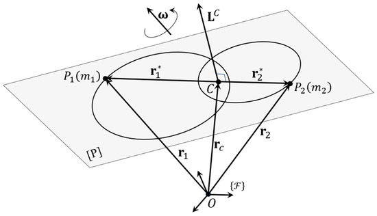
Figure 1. The trajectories are planar homothetical curves, situated on a variable plane, orthogonal to vector ${\mathbf{L}}^C$.

5.1.3. The Laws of the Motion of Particles in the Non-Inertial Reference Frame

From Equations (101) and (111), it follows that

$$\left\{\begin{array}{l}{\mathbf{r}}_1\left(t\right)={\mathbf{r}}_C\left(t\right)-{\displaystyle \frac{m_2}{m_1+m_2}}\mathbf{r}\left(t\right); \\ {\mathbf{r}}_2\left(t\right)={\mathbf{r}}_C\left(t\right)+{\displaystyle \frac{m_1}{m_1+m_2}}\mathbf{r}\left(t\right).\end{array}\right.$$

(120)

The vector function ${\mathbf{r}}_C\left(t\right)$ is the solution to IVP (103), and it has the explicit expression given in Equation (103). The vector function $\mathbf{r}\left(t\right)$ is the solution to IVP (116).

5.1.4. The Gravitational Two-Body Problem in a Non-Inertial Reference Frame: An Exact Closed-Form Solution

In the case of a gravitational two-body problem in a non-inertial reference frame, the laws of motion of the two particles (see Equations (105) and (106)) can be determined in closed-form coordinate-free solutions. The barycenter is due to Equation (103), and the relative motion is the subject of IVP (116)

The exact solution to the problem (116) is obtained (see Lemma 5) by applying the tensor ${\mathbf{R}}_{-\mathsf{\omega }}$ to the solution to Kepler’s problem:

$$\left\{\begin{array}{l}\ddot{\mathbf{r}}+{\displaystyle \frac{\mu }{{\mathrm{r}}^2}}\widehat{\mathit{r}}=\mathbf{0},\\ \left\{\begin{array}{l}\mathbf{r}\left(t_0\right)={\mathbf{r}}^0\\ \dot{\mathbf{r}}\left(t_0\right)={\mathbf{v}}^0+{\mathsf{\omega }}^0\times {\mathbf{r}}^0\end{array}\right.\end{array}\right.$$

(121)

Let the first integrals of the Kepler problem (121) be thus [37,38,39,40]:

Specific energy:

$$\xi ={\displaystyle \frac{1}{2}}{‖\dot{\mathbf{r}}‖}^2-{\displaystyle \frac{\mu }{‖\mathbf{r}‖}}={\displaystyle \frac{1}{2}}{‖{\mathbf{v}}^0+{\mathsf{\omega }}^0\times {\mathbf{r}}^0‖}^2-{\displaystyle \frac{\mu }{‖{\mathbf{r}}^0‖}}$$

(122)

Specific angular momentum:

$$\mathbf{h}=\mathbf{r}\times \dot{\mathbf{r}}={\mathbf{r}}^0\times \left[{\mathbf{v}}^0+{\mathsf{\omega }}^0\times {\mathbf{r}}^0\right].$$

(123)

Eccentricity vector:

$$\mathbf{e}={\displaystyle \frac{1}{\mu }}\dot{\mathbf{r}}\times \mathbf{h}-{\displaystyle \frac{\mathbf{r}}{‖\mathbf{r}‖}}={\displaystyle \frac{1}{\mu }}\left[{\mathbf{v}}^0+{\mathsf{\omega }}^0\times {\mathbf{r}}^0\right]\times \mathbf{h}-{\displaystyle \frac{{\mathbf{r}}^0}{‖{\mathbf{r}}^0‖}}.$$

(124)

In this case, the trajectories are in the rotating plan of the barycenter (see Figure 1). In this plan, trajectories are homothetical ellipses ($\xi <0$), homothetical parabolas ($\xi =0$), or homothetical hyperbolas ($\xi >0$). The non-collision sufficient condition is $\mathbf{h}\ne \mathbf{0}$. The collision necessary condition is $\mathbf{h}=\mathbf{0}$. The sufficient escape condition is $\mathbf{h}\ne \mathbf{0}$, $\xi \ge 0$.

If $\xi \ne \mathbf{0}$, and $\mathbf{h}\ne \mathbf{0}$, it denotes $n={\displaystyle \frac{\mu }{{\left(2\left|\xi \right|\right)}^{\frac{3}{2}}}}$ and the vectorial orbital elements of Kepler problem [39] are

$$\mathbf{a}=\left\{\begin{array}{c}{\displaystyle \frac{\mu }{2\mathrm{e}\left|\xi \right|}}\mathbf{e}, \mathbf{e}\ne \mathbf{0}\\ {\mathbf{r}}_c^0+{\mathbf{r}}_0, \mathbf{e}=\mathbf{0}\end{array}\right.$$

(125)

$$\mathbf{b}=\left\{\begin{array}{c}{\displaystyle \frac{1}{\mathrm{e}\sqrt{2\left|\xi \right|}}} \mathbf{h}\times \mathbf{e}, \mathbf{e}\ne \mathbf{0}\\ {\displaystyle \frac{1}{n}}\left[{\mathbf{v}}^0+{\mathsf{\omega }}^0\times {\mathbf{r}}^0\right], \mathbf{e}=\mathbf{0}\end{array},\right.$$

(126)

If it is the case that $\mathbf{h}\ne \mathbf{0}$,

(a)

if $\xi <\mathbf{0}$, the closed-form, coordinate-free solution of IVP (116) is given:

$$\mathbf{r}=\left[\mathrm{c}\mathrm{o}\mathrm{s}E\left(t\right)-e\right]{\mathbf{R}}_{-\mathsf{\omega }}\mathbf{a}+\left[\mathrm{s}\mathrm{i}\mathrm{n}E\left(t\right)\right]{\mathbf{R}}_{-\mathsf{\omega }}\mathbf{b}; t\ge t_0$$

(127)

The eccentric anomaly $E\left(t\right)$ is given by the Kepler equation:

$$E\left(t\right)-e\mathrm{s}\mathrm{i}\mathrm{n}\left[E\left(t\right)\right]=n\left(t-t_p\right)$$

(128)

$$t_p=t_0-{\displaystyle \frac{1}{n}}{(E}_o-e\mathrm{s}\mathrm{i}\mathrm{n}{E}_o)$$

(129)

$$E_o=\mathrm{a}\mathrm{t}\mathrm{a}\mathrm{n}2\left[n{\displaystyle \frac{{\mathbf{v}}^0·{\mathbf{r}}^0}{2\left|\xi \right|}}, 1-n{\displaystyle \frac{‖{\mathbf{r}}^0‖}{\sqrt{2\left|\xi \right|}}}\right]$$

(130)

(b)

If $\xi =0$, the closed-form, coordinate-free solution of IVP (116) is given:

$$\mathbf{r}={\displaystyle \frac{1}{2}}\left[{\displaystyle \frac{{\mathbf{h}}^2}{\mu }}+\mu {\tau }^2\left(t\right)\right]{\mathbf{R}}_{-\mathsf{\omega }}\mathbf{e}+\tau \left(t\right){\mathbf{R}}_{-\mathsf{\omega }}\left(\mathbf{h}\times \mathbf{e}\right); t\ge t_0$$

(131)

In Equation (131), ${\mathbf{h}}^2={‖\mathbf{h}‖}^2$ and $\tau \left(t\right)$ are the solution to the parabolic Kepler equation:

$$t-t_p={\displaystyle \frac{1}{2}}\left[{\displaystyle \frac{{\mathbf{h}}^2}{\mu }}\tau \left(t\right)+\mu {\displaystyle \frac{{\tau }^3\left(t\right)}{3}}\right]$$

(132)

where

$$t_p=t_0-{\displaystyle \frac{{\mathbf{v}}^0·{\mathbf{r}}^0}{2\mu }}\left[{\displaystyle \frac{{\mathbf{h}}^2}{\mu }}+{\displaystyle \frac{({{\mathbf{v}}^0·{\mathbf{r}}^0)}^2}{3\mu }}\right]$$

(133)

(c)

For $\mathsf{\xi }>0$, the closed-form, coordinate-free solution of IVP (116) is given:

$$\mathbf{r}=\left[e-\mathrm{c}\mathrm{o}\mathrm{s}\mathrm{h}E\left(t\right)\right]{\mathbf{R}}_{-\mathsf{\omega }}\mathbf{a}+\left[\mathrm{s}\mathrm{i}\mathrm{n}\mathrm{h}E\left(t\right)\right]{\mathbf{R}}_{-\mathsf{\omega }}\mathbf{b}; t\ge t_0$$

(134)

where $E\left(t\right)$ is definite by the functional equation (hyperbolic Kepler equation):

$$e\mathrm{s}\mathrm{i}\mathrm{n}\mathrm{h}\left[E\left(t\right)\right]-E\left(t\right)=n\left(t-t_0\right)+e\mathrm{s}\mathrm{i}\mathrm{n}\mathrm{h} E_o-E_o,$$

(135)

$$E_o={sinh}^{-1}\left[n{\displaystyle \frac{{\mathbf{v}}^0·{\mathbf{r}}^0}{2\mathrm{e}\xi }} \right]$$

(136)

If it is the case that $\mathbf{h}=\mathbf{0}$,

(a)

If $\xi <0$, the closed-form, coordinate-free solution of IVP (116) is given:

$$\mathbf{r}=\mathrm{a}\left[1-\mathrm{c}\mathrm{o}\mathrm{s}E\left(t\right)\right]{\mathbf{R}}_{-\mathsf{\omega }}{\displaystyle \frac{{\mathbf{r}}^0}{‖{\mathbf{r}}^0‖}}$$

(137)

where $\mathrm{a}={\displaystyle \frac{\mu }{2\left|\xi \right|}}$, and the $E\left(t\right)$ is given by the Kepler equation:

$$E\left(t\right)-\mathrm{s}\mathrm{i}\mathrm{n}\left[E\left(t\right)\right]=n\left(t-t_p\right)$$

(138)

$$t_p=t_0-{\displaystyle \frac{1}{n}}{(E}_o-\mathrm{s}\mathrm{i}\mathrm{n}{E}_o)$$

(139)

$$E_o=\mathrm{a}\mathrm{t}\mathrm{a}\mathrm{n}2\left[n{\displaystyle \frac{{\mathbf{v}}^0·{\mathbf{r}}^0}{2\left|\xi \right|}}, 1-n{\displaystyle \frac{‖{\mathbf{r}}^0‖}{\sqrt{2\left|\xi \right|}}}\right]$$

(140)

The motion is an inevitably a collision. If Equation (137) works for $t\in \left[t_0,t_c\right]$, the moment of collision is

$$t_c=t_0-{\displaystyle \frac{1}{n}}{(E}_o-\mathrm{s}\mathrm{i}\mathrm{n}{E}_o)+{\displaystyle \frac{2\pi }{n}}$$

(141)

(b)

If $\xi =0$, the closed-form, coordinate-free solution of IVP (116) is given:

$$\mathbf{r}={\displaystyle \frac{1}{2}}\left[\mu {\tau }^2\left(t\right)\right]{\mathbf{R}}_{-\mathsf{\omega }}{\displaystyle \frac{{\mathbf{r}}^0}{‖{\mathbf{r}}^0‖}}$$

(142)

In Equation (142), $\tau \left(t\right)$ is the solution to the parabolic Kepler equation:

$$t-t_p={\displaystyle \frac{1}{2}}\left[\mu {\displaystyle \frac{{\tau }^3\left(t\right)}{3}}\right],$$

(143)

where

$$t_p=t_0-\left[{\displaystyle \frac{({{\mathbf{v}}^0·{\mathbf{r}}^0)}^3}{6{\mu }^2}}\right]$$

(144)

The motion is an escape if ${\mathbf{v}}^0·{\mathbf{r}}^0>0$. The equation (151) works for $t\in [t_0,\infty )$.

The motion is a collision if ${\mathbf{v}}^0·{\mathbf{r}}^0<0$, and the moment of collision is $t_c=t_p=t_0-\left[{\displaystyle \frac{({{\mathbf{v}}^0·{\mathbf{r}}^0)}^3}{6{\mu }^2}}\right]$

(c)

For $\xi >0$, the closed-form, coordinate-free solution of IVP (116) is given:

$$\mathbf{r}=\mathrm{a}\left[\mathrm{c}\mathrm{o}\mathrm{s}\mathrm{h}E\left(t\right)-1\right]{\mathbf{R}}_{-\mathsf{\omega }}{\displaystyle \frac{{\mathbf{r}}^0}{‖{\mathbf{r}}^0‖}}$$

(145)

where $a={\displaystyle \frac{\mu }{2\xi }}$ and $E\left(t\right)$ is definite by the functional equation (hyperbolic Kepler equation):

$$\mathrm{s}\mathrm{i}\mathrm{n}\mathrm{h}\left[E\left(t\right)\right]-E\left(t\right)=n\left(t-t_0\right)+\mathrm{s}\mathrm{i}\mathrm{n}\mathrm{h} E_o-E_o,$$

(146)

$$E_o={sinh}^{-1}\left(n{\displaystyle \frac{{\mathbf{v}}^0·{\mathbf{r}}^0}{2\xi }}\right)$$

(147)

The motion is an escape if ${\mathbf{v}}^0·{\mathbf{r}}^0>0$. Equation (145) works for $t\in [t_0,\infty )$.

The motion is a collision if ${\mathbf{v}}^0·{\mathbf{r}}^0<0$. Equation (145) works for t $t\in [t_0,t_c)$, the moment of collision is

$$t_c=t_0-{\displaystyle \frac{1}{n}}\left[n{\displaystyle \frac{{\mathbf{v}}^0·{\mathbf{r}}^0}{2\xi }}-{\mathrm{s}\mathrm{i}\mathrm{n}\mathrm{h}}^{-1}\left(n{\displaystyle \frac{{\mathbf{v}}^0·{\mathbf{r}}^0}{2\xi }}\right)\right].$$

(148)

The laws of motion of the gravitational two-body problem in a general non-inertial reference frame, given by IVPs (99) and (100), are obtained via Equations (103), (120), (127), (131), and (134) and (137), (142), and (145), respectively. The exact solutions are closed-form and coordinate-free. To the author’s knowledge, this comprehensive approach is given for the first time in this paper.

5.2. Relative Orbital Motion of Spacecraft: A Closed-Form Coordinate-Free Solution

The relative orbital motion of spacecraft is a foundational issue in the field of astrodynamics, with numerous applications, including rendezvous operations, distributed spacecraft missions, and formation flying. Some notable applications of formation-flying spacecraft include space-based radar, ground-based terrestrial laser communication systems, Earth surveillance, remote sensing, stellar imaging, and astrometry.

Within the relative orbital motion model, two spacecraft (denoted as Chief and Deputy, respectively) are shown to fly in Keplerian orbits around the same gravitational center. The primary challenge in this model is determining the motion of the Deputy spacecraft within a local vertical local horizontal (LVLH) non-inertial frame that originates from the center of mass of the Chief spacecraft.

The position vector of Chief’s mass center, denoted by ${\mathbf{r}}_c$, originates in the gravitational attracting center. In the LVLH non-inertial reference frame,

$${\mathbf{r}}_c={\displaystyle \frac{p_c}{1+e_{c}cos{f}_c\left(t\right)}}{\displaystyle \frac{{\mathbf{r}}_c^0}{‖{\mathbf{r}}_c^0‖}}.$$

(149)

In Equation (149), ${\mathbf{r}}_c^0={\mathbf{r}}_c\left(t_0\right)$, $p_c$ is the semi-latus conic parameter, $e_c$ is the eccentricity, and $f_c=f_c\left(t\right)$ is the true anomaly of the Chief spacecraft. The unit orthogonal basis of the LVLF frame is ${\mathbf{u}}_x={\displaystyle \frac{{\mathbf{r}}_c^0}{‖{\mathbf{r}}_c^0‖}}$, ${\mathbf{u}}_z={\displaystyle \frac{{\mathbf{h}}_c}{‖{\mathbf{h}}_c‖}}$, and ${\mathbf{u}}_y={\mathbf{u}}_z\times {\mathbf{u}}_x$, where ${\mathbf{h}}_c$ denotes the specific angular momentum of the Chief spacecraft.

By time differentiable of ${\mathbf{r}}_c$ in the LVLH frame is

$${\dot{\mathbf{r}}}_c={\displaystyle \frac{e_c‖{\mathbf{h}}_c‖sin{f}_c\left(t\right)}{p_c}}{\displaystyle \frac{{\mathbf{r}}_c^0}{‖{\mathbf{r}}_c^0‖}}.$$

(150)

The instantaneous angular velocity of the non-inertial reference frame LVLH is given by the following equation:

$${\mathsf{\omega }}_c=\dot{f_c}{\mathbf{u}}_z={\displaystyle \frac{1}{{\mathbf{r}}_c^2}}{\mathbf{h}}_c={{\displaystyle \frac{[1+e_{c}cos{f}_c\left(t\right)]}{{\mathrm{p}}_c^2}}}^2{\mathbf{h}}_c,$$

(151)

and has a fixed direction vector function of time.

For t $=t_0$, denote ${\dot{\mathbf{r}}}_c\left(t_0\right)={\dot{\mathbf{r}}}_c^0$ and ${\mathsf{\omega }}_c\left(t_0\right)={\mathsf{\omega }}_c^0$:

$${\dot{\mathbf{r}}}_c^0={\displaystyle \frac{e_c‖{\mathbf{h}}_c‖sin{f}_c\left(t_0\right)}{p_c}}{\displaystyle \frac{{\mathbf{r}}_c^0}{‖{\mathbf{r}}_c^0‖}},$$

(152)

$${\mathsf{\omega }}_c^0={{\displaystyle \frac{[1+e_{c}cos{f}_c\left(t_0\right)]}{{\mathrm{p}}_c^2}}}^2{\mathbf{h}}_c.$$

(153)

The relative motion of the Deputy spacecraft in a non-inertial LVLH reference frame is given by the following IVP:

$$\left\{\begin{array}{l}\ddot{\mathbf{r}}+2{\mathsf{\omega }}_c\times \dot{\mathbf{r}}+{\mathsf{\omega }}_c\times \left({\mathsf{\omega }}_c\times \mathbf{r}\right)+{\dot{\mathsf{\omega }}}_c\times \mathbf{r}+{\mathbf{a}}_c={\mathbf{a}}_g\\ \left\{\begin{array}{l}\mathbf{r}\left(t_0\right)={\mathbf{r}}_0\\ \dot{\mathbf{r}}\left(t_0\right)={\mathbf{v}}_0\end{array}\right.\end{array}\right.$$

(154)

In Equation (154), ${\mathbf{a}}_c$ and ${\mathbf{a}}_g$ are ($\mu$ is a gravitational parameter of the attraction center):

$${\mathbf{a}}_c=-{\displaystyle \frac{\mu }{{‖{\mathbf{r}}_C‖}^3}}{\mathbf{r}}_c,$$

(155)

$${\mathbf{a}}_g=-{\displaystyle \frac{\mu }{{‖{\mathbf{r}+\mathbf{r}}_C‖}^3}}\left({\mathbf{r}+\mathbf{r}}_c\right),$$

(156)

the position vector of the Deputy mass center in the LVLH frame is ${\mathbf{r}}_0$, and its relative velocity is ${\mathbf{v}}_0$.

Equation (154) considers the effects of Coriolis, Euler, centrifugal and translational inertial forces in the general non-inertial reference LVLH frame.

Thus, the relative orbital motion is described by this IVP:

$$\left\{\begin{array}{l}\ddot{\mathbf{r}}+2{\mathsf{\omega }}_c\times \dot{\mathbf{r}}+{\mathsf{\omega }}_c\times \left({\mathsf{\omega }}_c\times \mathbf{r}\right)+{\dot{\mathsf{\omega }}}_c\times \mathbf{r}+{\displaystyle \frac{\mu }{{‖{\mathbf{r}+\mathbf{r}}_c‖}^3}}\left({\mathbf{r}+\mathbf{r}}_c\right)-{\displaystyle \frac{\mu }{{‖{\mathbf{r}}_c‖}^3}}{\mathbf{r}}_c=\mathbf{0}\\ \left\{\begin{array}{l}\mathbf{r}\left(t_0\right)={\mathbf{r}}_0\\ \dot{\mathbf{r}}\left(t_0\right)={\mathbf{v}}_0\end{array}\right.\end{array}\right.$$

(157)

By change of variable ${\mathbf{r}}_{\ast }={\mathbf{F}}_{{\mathsf{\omega }}_c}(\mathbf{r}+{\mathbf{r}}_c)$, after some algebra, Lemma 3, Lemma 4, and Equation (157) result:

$$\left\{\begin{array}{l}\ddot{{\mathbf{r}}_{\ast }}+{\displaystyle \frac{\mu }{{\mathrm{r}}_{\mathrm{*}}^2}}{\widehat{\mathbf{r}}}_{\ast }=\mathbf{0},\\ \left\{\begin{array}{l}{\mathbf{r}}_{\ast }\left(t_0\right)={\mathbf{r}}_{\ast }^0\\ \dot{{\mathbf{r}}_{\ast }}\left(t_0\right)={\mathbf{v}}_{\ast }^0\end{array}\right.\end{array}\right.,$$

(158)

Denote:

$${\mathbf{r}}_{\ast }^0={\mathbf{r}}_0+{\mathbf{r}}_c^0,$$

(159)

$${\mathbf{v}}_{\ast }^0={\mathbf{v}}_0+{\dot{\mathbf{r}}}_c^0+{\mathsf{\omega }}_c^0\times ({\mathbf{r}}_0+{\mathbf{r}}_c^0)$$

(160)

It thus follows that the unique solution of the orbital relative motion, modelled by IVP (157), is given by

$$\mathbf{r}={\mathbf{R}}_{-{\mathsf{\omega }}_c}{\mathbf{r}}_{\ast }-{\displaystyle \frac{p_c}{1+e_{c}cos{f}_c\left(t\right)}}{\displaystyle \frac{{\mathbf{r}}_c^0}{‖{\mathbf{r}}_c^0‖}},$$

(161)

where (see Appendix A.2)

$${\mathbf{R}}_{-{\mathsf{\omega }}_c}={\mathbf{I}}_3-{\displaystyle \frac{1}{‖{\mathbf{h}}_c‖}}\sin \left[f_c\left(t\right)-f_c\left(t_0\right)\right]\widetilde{{\mathbf{h}}_c}+{\displaystyle \frac{1}{{‖{\mathbf{h}}_c‖}^2}}\left[1-\cos \left[f_c\left(t\right)-f_c\left(t_0\right)\right]\right]{\widetilde{{\mathbf{h}}_c}}^2.$$

(162)

The solution of the vectorial Kepler problem (158) was presented comprehensively in the previous section. For details, see [40,41,42,43,44,45].

6. Conclusions

This paper addresses the N-body problem in an arbitrary non-inertial reference frame for the first time. It presents first integrals, like those in the inertial case, using appropriate mathematical tools. The first integrals of motion are extended to encompass the general case of the N-body problem in a non-inertial reference frame and the barycenter system of particles. For the two-body problem, the paper provides coordinate-free closed-form solutions for the equations of motion in an arbitrary non-inertial frame. It also identifies new sufficient conditions for stability against impact and relative equilibrium in the two-body problem. A comprehensive approach to the gravitational two-body problem in a general non-inertial reference frame is detailed, along with a complete solution for the relative orbital motion of spacecraft. The prime integrals presented demonstrate geometric and energy significance in the general and specific cases discussed. In future work, new Sundman-type inequalities will be employed to qualitatively analyze the N-body problem in a non-inertial reference frame, focusing on Lagrange and Hill stability, collision scenarios, and sufficient escape conditions.

Appendix A.1. The Proof of Lemma 1

From the existence and uniqueness theorem, it follows that IVP (1) has a unique solution $\mathbf{Q}=\mathbf{Q}\left(t\right)$. The Euclidean tensor $\mathbf{Q}$ is in $\mathbf{S}{\mathbf{O}}_3^{\mathbb{R}}$, if and only if ${\mathbf{Q}}^{\mathrm{T}}\mathbf{Q}={\mathbf{I}}_3$ and $det\left(\mathbf{Q}\right)=1$ By differentiating the condition ${\mathbf{Q}}^{\mathrm{T}}\mathbf{Q}={\mathbf{I}}_3$: ${\displaystyle \frac{d}{dt}}\left(\mathbf{Q}{\mathbf{Q}}^{\mathrm{T}}\right)=\dot{\mathbf{Q}}{\mathbf{Q}}^{\mathrm{T}}+\mathbf{Q}{\dot{\mathbf{Q}}}^{\mathrm{T}}=\mathbf{Q}\tilde{\mathsf{\omega }}{\mathbf{Q}}^{\mathrm{T}}-\mathbf{Q}\tilde{\mathsf{\omega }}{\mathbf{Q}}^{\mathrm{T}}=0_3$ so $\mathbf{Q}{\mathbf{Q}}^{\mathrm{T}}$ is a constant function and $\mathbf{Q}{\mathbf{Q}}^{\mathrm{T}}\left(t_0\right)={\mathbf{I}}_3$. This tensorial function is continuous which satisfies $\mathrm{d}\mathrm{e}\mathrm{t}\left(\mathbf{Q}\right)\in \left\{-\mathrm{1,1}\right\}$ and $\mathrm{d}\mathrm{e}\mathrm{t}\left(\mathbf{Q}\left(t_0\right)\right)=\mathrm{d}\mathrm{e}\mathrm{t}{\mathbf{I}}_3=1$, it follows that $det\left(\mathbf{Q}\right)=1.$

Appendix A.2. Closed-Form Solution of Kinematic Equation

Initial value tensorial equation by Equation (3) is:

$${\dot{\mathbf{R}}}_{-\mathsf{\omega }}+\tilde{\mathsf{\omega }}{\mathbf{R}}_{-\mathsf{\omega }}=\mathbf{0}; {\mathbf{R}}_{-\mathsf{\omega }}\left(t_0\right)={\mathbf{I}}_3.$$

(A1)

This is differential first-order linear equation time-variable. Is known as the Peano-Baker solution, it is obtained by iteration [34,35,37,38,39,40] and it is presented as a limit of infinitesimal integrals:

$${\mathbf{R}}_{-\mathsf{\omega }}\left(t\right)={\mathbf{I}}_3+\sum _{n=1}^{\mathrm{\infty }}{\displaystyle \frac{1}{n!}}\underset{t_0}{\overset{t}{\int }}d{t}_1\dots \underset{t_0}{\overset{t}{\int }}d{t}_n\mathbf{T}\left[\tilde{\mathsf{\omega }}\left(t_1\right),\dots ,\tilde{\mathsf{\omega }}\left(t_n\right)\right],$$

(A2)

with

$$\mathbf{T}\left[\tilde{\mathsf{\omega }}\left(t_1\right),\dots ,\tilde{\mathsf{\omega }}\left(t_n\right)\right]\triangleq {\displaystyle \frac{{\left(-1\right)}^n}{2^n}}\sum _{\sigma \in \mathcal{P}\left(n\right)}\left[\prod _{k=1}^{n-1}\mathsf{\theta }\left(t_{\sigma \left(k\right)}\right.-\left.t_{\sigma \left(k+1\right)}\right)\prod _{p=1}^n\tilde{\mathsf{\omega }}\left(t_{\sigma \left(p\right)}\right)\right],$$

(A3)

$$\mathsf{\theta }\left(t\right)=\left\{\begin{array}{l}0,t\le t_0\\ 1,t>t_0\end{array}\right.,$$

(A4)

In Equation (A3), $\mathcal{P}\left(n\right)$ denotes the group of permutations of the set $\left\{1,\dots ,n\right\},n>2$.

• If instantaneous angular velocity $\mathsf{\omega }$ has fixed direction, $\mathsf{\omega }=\mathsf{\omega }\left(t\right)\mathbf{u}$, with $\mathbf{u}$ being the constant unit vector and $\mathsf{\omega }:\mathbb{R}\to \mathbb{R}$ a real function, since $\tilde{\mathsf{\omega }}\left(t_1\right)\tilde{\mathsf{\omega }}\left(t_2\right)=\tilde{\mathsf{\omega }}\left(t_2\right)\tilde{\mathsf{\omega }}\left(t_1\right)$, $\left(\forall \right)t_{\mathrm{1,2}}\in \mathbb{R}$, (also see Refs. [20,21]), then ${\mathbf{R}}_{-\mathsf{\omega }}$ has the time explicit expression:

$${\mathbf{R}}_{-\mathsf{\omega }}\left(t\right)=\mathrm{e}\mathrm{x}\mathrm{p}\left(-\underset{t_0}{\overset{t}{\int }}\tilde{\mathsf{\omega }}\left(s\right)\mathrm{d}s\right)={\mathbf{I}}_3-\mathrm{s}\mathrm{i}\mathrm{n}\phi \left(t\right)\tilde{\mathbf{u}}+\left[1-\mathrm{c}\mathrm{o}\mathrm{s}\phi \left(t\right)\right]{\tilde{\mathbf{u}}}^2,$$

(A5)

will denote

$$\phi \left(t\right)=\underset{t_0}{\overset{t}{\int }}\mathsf{\omega }\left(s\right)\mathrm{d}s.$$

(A6)

• If instantaneous angular velocity ω is constant vector, then ${\mathbf{R}}_{-\mathsf{\omega }}$ has the time explicit expression:

$${\mathbf{R}}_{-\mathsf{\omega }}\left(t\right)=\mathrm{e}\mathrm{x}\mathrm{p}\left[-\left(t-t_0\right)\tilde{\mathsf{\omega }}\right]={\mathbf{I}}_3-\mathrm{s}\mathrm{i}\mathrm{n}\left[\mathsf{\omega }\left(t-t_0\right)\right]\widehat{\mathsf{\omega }}+\left\{1-\mathrm{c}\mathrm{o}\mathrm{s}\left[\mathsf{\omega }\left(t-t_0\right)\right]\right\}{\left(\widehat{\mathsf{\omega }}\right)}^2.$$

(A7)

• If vector $\mathsf{\omega }$ has a regular precession with angular velocity ${\mathsf{\omega }}_1$ around a fixed axis, expressed like:

$$\begin{array}{l}\mathsf{\omega }={\mathbf{R}}_1{\mathsf{\omega }}_0; \\ {\mathsf{\omega }}_0=\mathsf{\omega }\left(t_0\right); \\ {\mathbf{R}}_1=\mathrm{e}\mathrm{x}\mathrm{p}\left[\left(t-t_0\right){\tilde{\mathsf{\omega }}}_1\right],\end{array}$$

(A8)

then the IVP (3) still has a time–explicit solution [20,21], expressed:

$${\mathbf{R}}_{-\mathsf{\omega }}\left(t\right)=\mathrm{e}\mathrm{x}\mathrm{p}\left[\left(t-t_0\right){\tilde{\mathsf{\omega }}}_1\right]\mathrm{e}\mathrm{x}\mathrm{p}\left[-\left(t\right.\right.-\left.t_0\right)\left.\left({\tilde{\mathsf{\omega }}}_1+{\tilde{\mathsf{\omega }}}_0\right)\right],$$

(A9)

and is written in closed form:

$$\begin{array}{l}{\mathbf{R}}_{-\mathsf{\omega }}=\left\{{\mathbf{I}}_3+\mathrm{s}\mathrm{i}\mathrm{n}\left[{\mathsf{\omega }}_1\left(t-t_0\right)\right]{\widehat{\mathsf{\omega }}}_1+\left\{1-\mathrm{c}\mathrm{o}\mathrm{s}\left[{\mathsf{\omega }}_1\left(t-t_0\right)\right]\right\}{\left({\widehat{\mathsf{\omega }}}_1\right)}^2\right\}\times \\ \times \left\{{\mathbf{I}}_3-\mathrm{s}\mathrm{i}\mathrm{n}\left[{\mathsf{\omega }}_2\left(t-t_0\right)\right]{\widehat{\mathsf{\omega }}}_2+\left\{1-\mathrm{c}\mathrm{o}\mathrm{s}\left[{\mathsf{\omega }}_2\left(t-t_0\right)\right]\right\}{\left({\widehat{\mathsf{\omega }}}_2\right)}^2\right\},\end{array}$$

(A10)

where:

$${\mathsf{\omega }}_2={\mathsf{\omega }}_1+{\mathsf{\omega }}_0.$$

(A11)

• A comprehensive study, together with a closed-form solution to the kinematic equation in the general case, may be found in Ref. [37]

Remark A1.

Equations (A5), (A7) and (A10) present the closed-form solution to the kinematics equation in scenarios where the instantaneous angular velocity vector has a fixed direction, remains constant, or exhibits regular precession.

References

- Poincare, H. New Methods of Celestial Mechanics; Goroff, D.L., Ed.; American Institute of Physics: New York, NY, USA, 1993. [Google Scholar]
- Saari, D.G. A Visit to the Newtonian N-Body Problem via Elementary Complex Variables. Am. Math. Mon. 1990, 97, 105–119. [Google Scholar] [CrossRef]
- Saari, D.G. Collisions, Rings, and Other Newtonian N-Body Problems; CBMS Regional Conference Series in Mathematics; American Mathematical Society: Providence, RI, USA, 2005. [Google Scholar] [CrossRef]
- Sundman, K. Recherches sur le problème des trois corps. Acta Soc. Sci. Fenn. 1907, 34. [Google Scholar]
- Sundman, K.F. Nouvelles recherches sur le problème des trois corps. Acta Soc. Sci. Fenn. 1909, 35. [Google Scholar]
- Sundman, K. Mémoire sur le problème des trois corps. Acta Math. 1912, 36, 105–179. [Google Scholar] [CrossRef]
- Wang, Q. The Global Solution of the N-Body Problem. Celest. Mech. 1991, 50, 73–88. [Google Scholar] [CrossRef]
- Diacu, F.; Stoica, C.; Zhu, S. Central Configurations of the Curved N-Body Problem. J. Nonlinear Sci. 2018, 28, 1999–2046. [Google Scholar] [CrossRef]
- Scheeres, D.J. Relative Equilibria in the Full N-Body Problem with Applications to the Equal Mass Problem. In Recent Advances in Celestial and Space Mechanics; Springer: Cham, Switzerland, 2016; p. 23. [Google Scholar] [CrossRef]
- Scheeres, D.J. Stability in the Full Two-Body Problem. Celest. Mech. Dyn. Astron. 2002, 83, 155–169. [Google Scholar] [CrossRef]
- Scheeres, D.J. Relative Equilibria for General Gravity Fields in the Sphere-Restricted Full 2-Body Problem. Celest. Mech. Dyn. Astron. 2006, 94, 317–349. [Google Scholar] [CrossRef]
- Scheeres, D.J. Minimum Energy Configurations in the N-Body Problem and the Celestial Mechanics of Granular Systems. Celest. Mech. Dyn. Astron. 2012, 113, 291–320. [Google Scholar] [CrossRef]
- Scheeres, D.J. Hill Stability in the Full 3-Body Problem. Proc. Int. Astron. Union 2014, 9 (Suppl. S310), 134–137. [Google Scholar] [CrossRef]
- Scheeres, D.J. Stable and Minimum Energy Configurations in the Spherical, Equal Mass Full 4-Body Problem. Comput. Model. Eng. Sci. 2016, 111, 203–227. [Google Scholar] [CrossRef]
- Scheeres, D.J. Orbital Motion in Strongly Perturbed Environments; Springer: Berlin/Heidelberg, Germany, 2012. [Google Scholar] [CrossRef]
- Maciejewski, A.J. The Two Rigid Bodies Problem. Reduction and Relative Equilibria. In Hamiltonian Systems with Three or More Degrees of Freedom; Simó, C., Ed.; NATO ASI Series; Springer: Dordrecht, The Netherlands, 1999; Volume 533. [Google Scholar] [CrossRef]
- Polimeni, D.; Terracini, S. On the existence of minimal expansive solutions to the N-body problem. Invent. Math. 2024, 238, 585–635. [Google Scholar] [CrossRef]
- Ulibarrena, V.S.; Horn, P.; Portegies Zwart, S.; Sellentin, E.; Koren, B.; Cai, M.X. A hybrid approach for solving the gravitational N-body problem with Artificial Neural Networks. J. Comput. Phys. 2023, 496, 112596. [Google Scholar] [CrossRef]
- Boekholt, T.; Portegies Zwart, S. On the Reliability of N-body Simulations. Comput. Astrophys. Cosmol. 2015, 2, 2. [Google Scholar] [CrossRef]
- Szűcs-Csillik, I. Overview—Regularization and Numerical Methods in Celestial Mechanics and Dynamical Astronomy. Rom. Astron. J. 2023, 33, 37–56. [Google Scholar] [CrossRef]
- Longuski, J.M.; Hoots, F.R.; Pollock, G.E. The N-body Problem. In Introduction to Orbital Perturbations; Springer: Cham, Switzerland, 2021; pp. 1–17. [Google Scholar] [CrossRef]
- Di Ruzza, S. Classical and Relativistic N-body Problem: From Levi-Civita to the Most Advanced Interplanetary Missions. Eur. Phys. J. Plus 2021, 136, 1136. [Google Scholar] [CrossRef]
- Ershkov, S.; Leshchenko, D.; Prosviryakov, E.Y. Investigating the non-inertial R2BP in case of variable velocity of central body motion in a prescribed fixed direction. Arch. Appl. Mech. 2024, 94, 767–777. [Google Scholar] [CrossRef]
- Ershkov, S.; Leshchenko, D. Estimation of the size of the solar system and its spatial dynamics using Sundman inequality. Pramana J. Phys. 2022, 96, 158. [Google Scholar] [CrossRef]
- Ershkov, S.; Leshchenko, D. Analysis of the size of Solar system close to the state with zero total angular momentum via Sundman’s inequality. An. Acad. Bras. Ciências 2021, 93 (Suppl. S3), e20200269. [Google Scholar] [CrossRef] [PubMed]
- Ershkov, S.; Leshchenko, D.; Prosviryakov, E.Y. Illuminating dot-satellite motion around the natural moons of planets using the concept of ER3BP with variable eccentricity. Arch. Appl. Mech. 2024, 94, 515–527. [Google Scholar] [CrossRef]
- Aggarwal, R.; Mittal, A.; Suraj, M.S.; Bisht, V. The effect of small perturbations in the Coriolis and centrifugal forces on the existence of libration points in the restricted four-body problem with variable mass. Astron. Nachr. 2018, 339, 492–512. [Google Scholar] [CrossRef]
- Hallan, P.P.; Rana, N. Effect of perturbations in Coriolis and centrifugal forces on the location and stability of the equilibrium point in the Robe’s circular restricted three body problem. Planet. Space Sci. 2001, 49, 957. [Google Scholar] [CrossRef]
- Elipe, A.; da Costa, M.L.; Piccotti, L.; Tresaco, E. Close binary stars modelled by two prolate ellipsoids in synchronous rotation. Astron. J. 2024, 167, 25. [Google Scholar] [CrossRef]
- Efroimsky, M. Long-Term Evolution of Orbits About a Precessing Oblate Planet: 1. The Case of Uniform Precession. Celest. Mech. Dyn. Astr. 2005, 91, 75–108. [Google Scholar] [CrossRef]
- Efroimsky, M. Long-term evolution of orbits about a precessing oblate planet. 2. The case of variable precession. Celestial Mech. Dyn. Astr. 2006, 96, 259–288. [Google Scholar] [CrossRef][Green Version]
- Efroimsky, M.; Goldreich, P. Gauge freedom in the N-body problem of celestial mechanics. Astron. Astrophys. 2004, 415, 1187–1199. [Google Scholar] [CrossRef][Green Version]
- Condurache, D.; Martinusi, V. A Closed Form Solution of the Two Body Problem in Non-Inertial Reference Frames. Adv. Astronaut. Sci. 2012, 143, 1649–1668. [Google Scholar]
- Condurache, D. New Symbolic Procedures in the Study of the Dynamical Systems. Ph.D. Thesis, Technical University “Gheorghe Asachi”, Iasi, Romania, 1995. [Google Scholar]
- Fasano, A.; Marmi, S. Analytical Mechanics: An Introduction; Oxford University Press: Oxford, UK, 2006. [Google Scholar]
- Darboux, G. Leçons sur la Théorie Générale des Surfaces et Les Applications Géométriques du Calcul Infinitésimal; Gauthier-Villars: Paris, France, 1887; Volume 1. [Google Scholar]
- Condurache, D.; Martinusi, V. A Quaternionic Exact Solution to the Relative Orbital Motion Problem. J. Guid. Control Dyn. 2010, 30, 201–213. [Google Scholar] [CrossRef]
- Condurache, D.; Burlacu, A. Onboard Exact Solution to the Full-Body Relative Orbital Motion Problem. J. Guid. Control Dyn. 2016, 39, 2638–2648. [Google Scholar] [CrossRef]
- Condurache, D.; Martinuşi, V. A complete closed form vectorial solution to the Kepler problem. Meccanica 2007, 42, 465–476. [Google Scholar] [CrossRef]
- Condurache, D.; Martinusi, V. Kepler’s Problem in Rotating Reference Frames. Part 1: Prime Integrals, Vectorial Regularization. J. Guid. Control Dyn. 2007, 30, 192–200. [Google Scholar] [CrossRef]
- Condurache, D. N-Body Problem in Non-Inertial Reference Frame. Application to Full Two-Body Stability Problem. In Proceedings of the 73rd International Astronautical Congress, Astrodynamics Symposium, Paris, France, 18 September 2022; IAF: Paris, France. [Google Scholar]
- Condurache, D. Poisson-Darboux Problem’s Extended in Dual Lie Algebra. Adv. Astronaut. Sci. 2018, 162, 3345–3364. [Google Scholar]
- Condurache, D.; Martinusi, V. Relative Spacecraft Motion in A Central Force Field. J. Guid. Control Dyn. 2007, 30, 873–876. [Google Scholar] [CrossRef]
- Condurache, D.; Martinusi, V. Exact Solution to the Relative Orbital Motion in a Central Force Field. In Proceedings of the 2nd IEEE/AIAA International Symposium on Systems and Control in Aerospace and Astronautics, Shenzhen, China, 10–12 December 2008. [Google Scholar] [CrossRef]
- Condurache, D.; Martinusi, V. Foucault Pendulum-like Problems: A Tensorial Approach. Int. J. Non-Linear Mech. 2008, 43, 743–760. [Google Scholar] [CrossRef][Green Version]
Disclaimer/Publisher’s Note: The statements, opinions and data contained in all publications are solely those of the individual author(s) and contributor(s) and not of MDPI and/or the editor(s). MDPI and/or the editor(s) disclaim responsibility for any injury to people or property resulting from any ideas, methods, instructions or products referred to in the content. |
© 2025 by the authors. Licensee MDPI, Basel, Switzerland. This article is an open access article distributed under the terms and conditions of the Creative Commons Attribution (CC BY) license (https://creativecommons.org/licenses/by/4.0/).