Abstract
This study investigates overestimations in defect inspections performed by imperfect inspectors, particularly in scenarios involving random defective rates. Mathematical models are developed under two key assumptions: (1) inspection errors are either constant or uniformly distributed and (2) defective rates follow a random uniform distribution. Four analytical models are used to evaluate the probability of overestimation (PO) and identify critical defect rate thresholds (CFBs). The findings reveal that the PO approaches 100% as defect rates approach zero, irrespective of inspection error characteristics. Sensitivity analysis demonstrates model robustness under varying error distributions and parameter changes. Addressing practical concerns, this research highlights the need to revise inspection schemes to mitigate biases, especially in industries with stringent quality control standards, such as electronics and pharmaceuticals. Recommendations include integrating probabilistic error models and adopting dynamic calibration systems to improve inspection accuracy. By providing a theoretical foundation for tackling overestimation, this study has significant implications for improving fairness and efficiency in global supply chains.
1. Introduction
As an example, assume that there exists a batch of items with some defective rate (DR) whose constancy is unknown and is exposed to an imperfect inspector with nonzero inspection errors for the purpose of estimating the true value. This far-from-perfect inspector might be an automatic inspection machine. The inspector can have both a false high and a false low true defect rate (TDR). If a series of groups with heterogeneous DRs are presented to the inspector, the chance that the inspector overestimates, called the global probability of overestimation (PO), is calculated by taking the ratio of the number of overestimations recorded and the total number of groups diagnosed. In the early 2020s, a BLU manufacturer in Korea performed similar factory experiments and suggested an interpretation that imperfect inspectors are prone to overestimate the TDR if it is very low. Put simply, the inspector defective rate (IDR), the rate of defects detected by the inspector, might reliably exceed the TDR when the TDR is equal to zero. Should they be correct, the ramifications would likely require a revision of current inspection protocols. Also, if the PO is deemed necessary in traditional inspections for product “flawless” inspection, then traditional inspection methods will have to include the PO. The difficulty is proving their hypothesis in a coherent way. In order to prove or disprove their conjecture, various methodologies covering the statistical concepts of the PO and methods of PO computation would be required. To ensure mathematical rigor, the formal derivation and proofs of these properties are provided in Appendix A.
Since the 1970s, research on inspector errors has explored various aspects of quality control, including the effects of inspection errors on lot acceptance probability, average outgoing quality, and optimal inspection cycles. Collins et al. (1970), Dorris and Foote, Raz and Thomas, Tang, Lee, Duffuaa and Khan, and Yang and Cho examined different aspects of inspection errors, such as the impact of Type I and Type II errors on defect detection and strategies for optimizing inspection sequences [1,2,3,4,5,6,7]. Sylla and Drury [8] proposed the concept of inspector liability, analyzing how error-related payoffs and discriminability between noise and signal distributions influence quality decisions. Burk et al. [9] established a mathematical relationship between TDR and IDR, showing that for high-quality processes, IDR approaches Type I error as TDR decreases. Additionally, Yang [10] introduced a K-stage inspection-rework (K-IR) system and mathematically demonstrated that IDR always exceeds TDR under certain conditions, which highlighted the challenges of achieving accurate defect rate estimations in multi-stage inspections.
This issue of overestimating defective rates has continued to be a crucial research topic in the field of quality control. Recent studies have highlighted the significant impact of overestimation on various industrial settings. For instance, a hydrogen pipeline inspection study demonstrated how data-driven approaches can effectively address such overestimation issues while enhancing prediction accuracy [11].
The overestimation of defective rates by imperfect inspectors remains a significant challenge in quality control, especially in industries where maintaining extremely low defective rates (e.g., parts per million) is essential. For instance, in the BLU manufacturing industry, such overestimation can result in unnecessary financial losses, inefficiencies, and strained relationships in global supply chains. Addressing these challenges is critical to ensuring fairness and accuracy in international trade. This study developed a theoretical framework to better understand and mitigate overestimation, providing a foundation for revising inspection protocols.
Despite advancements, research addressing the systematic analysis of random defective rates and their influence on overestimation remains limited. While recent studies have proposed Bayesian models for inspection optimization [12] and examined the effects of inspection errors in inventory control [13,14], these approaches have primarily focused on specific applications such as rail systems and additive manufacturing. However, a more generalized probabilistic model applicable across diverse industries is still lacking. In an effort to mitigate inspection errors and enhance quality control, recent studies have integrated data-driven methodologies. Song et al. (2024) developed a data-driven quality prediction model incorporating uncertainty quantification to improve active sampling inspection in steel production. Their approach highlights the potential of leveraging uncertainty modeling to refine defect rate estimation. Inspired by such advancements, our research aims to systematically analyze the overestimation phenomenon using probabilistic models applicable to various industrial contexts [15].
In this context, recent studies have further emphasized the need for probabilistic models to address these inspection inaccuracies. Additionally, data-driven approaches, such as random forest models, have been adopted in manufacturing to enhance prediction accuracy and address quality control challenges [16].
For instance, Altay and Baykal-Gürsoy [12] developed a Bayesian model addressing the defect arrival rates in rail systems where zero-inflated miss rates affect inspection reliability. Their model offers insights into optimizing inspection schedules and maintenance to minimize the consequences of missed defects. Manna et al. [13] investigated the influence of inspection errors on inventory models, analyzing the implications of Type I and Type II errors on production results. Their research indicates that improving inspection and warranty strategies can help reduce the financial consequences of misidentified defects. Furthermore, Mokhtari and Asadkhani [14] extended economic order quantity models to include inspection errors, demonstrating that even small error rates can substantially reduce profits if not addressed with tailored strategies.
These recent research trends can be seen as further developments and extensions of the initial work by Yang and Chang [17], who were the first authors to study the overestimation conjecture from the factory perspective and proved statistically a significant theorem that the PO approaches 100% as the TDR approaches zero regardless of inspectors. Their research provided a fundamental understanding of the overestimation problem, and subsequent studies have built upon this foundation to develop models applicable to more complex situations and various industrial sectors.
In comparison with these past studies, our research extends Yang and Chang’s theorem by incorporating the case where TDR itself is treated as a random variable, allowing for a more generalized application of the model. While previous approaches have often been tailored to specific industries, such as rail systems or additive manufacturing, this study proposes an analytical framework that can be applied to broader manufacturing settings where defective rates are extremely low, and inspection errors are nonzero. By systematically analyzing the impact of TDR randomness on overestimation, our research provides new insights into improving defect rate estimation and refining quality control protocols in various industries.
2. Problem Statement
Yang and Chang [17] developed formulas for the IDR (the defect rate as determined by an imperfect inspector) and the likelihood of the inspector overestimating, given certain conditions. These conditions include an imperfect inspector with nonzero inspection errors evaluating an endless series of items one at a time, where the true defect rate (TDR) is constant q and unknown to the inspector. The formulas are as follows:
In these equations, i represents the number of inspected items. The term denotes the chance that the inspector incorrectly classifies the i-th conforming item as nonconforming and wrongly rejects it. Conversely, signifies the probability that the inspector mistakenly identifies the i-th nonconforming item as conforming and incorrectly accepts it.
This study incorporated the following premises:
- 1.
- The values were presumed to be either
- A fixed across all i or;
- Independently and identically distributed according to a uniform density function .
- 2.
- Similarly, the values were assumed to be either
- A constant for every i or;
- Independently and identically distributed according to a uniform density function .
- 3.
- The constants and were defined as and , respectively, with denoting the expected value of a random variable X.
Since a constant can be regarded as a random variable with zero variance, it follows that Equations (1) and (2) can be obtained, respectively, as
Sylla and Drury [8] defined the apparent nonconforming fraction as
Yang and Chang [17] described CF as a critical fraction defective (CF), defined as the critical defect rate at which the probability of overestimation or underestimation is exactly 50%. Mathematically, this is represented as or, equivalently, . Since the true defect rate (TDR) assumptions affect the derivation of both and CF, we use and CFC when the TDR is a constant q as well as and CFR when the TDR is a random variable Q with distribution for .
Based on their assumptions and results from four statistical models, they established the following theorem:
- 1.
- An imperfect inspector with has a unique curve with CF, where .
- 2.
- is a function of q and , denoted as .
- 3.
- decreases with q, reaching its maximum at and minimum at .
- 4.
- decreases with , with and .
- 5.
- A unique always exists, dependent only on inspection errors, not q.
- 6.
- The inspector overestimates q when for , accurately estimates q when for , and underestimates q when for .
The third statement indicates that approaches 100% as q nears 0%, regardless of . We aimed to determine if this theorem holds when he TDR follows the random variable Q distributed with . By substituting Q with q in Equations (3) and (4), we derive IDR and as
The under our assumptions should be expressed using input parameters , or , and or . However, as is a function of and (where ), we focus on the as a function of , and we use for simplicity. If a unique exists, where , it is termed “the critical DR bound” or the . The does not exist if and only if for . Since inspection errors A and B can be constant or random, we require four types of analysis for and , as illustrated in Table 1.

Table 1.
Four types of analysis with , , and . Input parameters and output results are clearly separated.
This research problem can be concisely stated as follows: derive and for each model and address the fundamental question: does their theorem remain valid when the TDR itself is a random variable?
3. Analysis of Model R-I (C, C)
The key input and output variables for Model R-I are summarized in Table 2. Consider the scenario where and , with and being constants. Given that and can be interpreted as and , respectively, the correlation coefficient can be calculated as
Table 2.
Key input and output variables for Model R-I.
The subsequent proposition demonstrates that the characteristic form of changes based on the value of , as illustrated in Figure 1. Additionally, the critical fraction bound is given by
which depends solely on and exists only when (refer to Figure 1b,c). It is noteworthy that
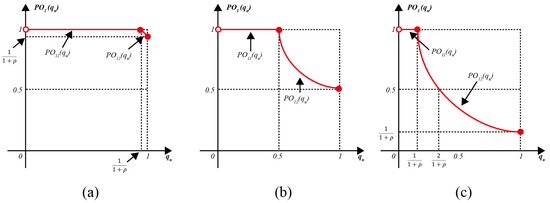
Figure 1.
Three representative graphs of depending on the value of : (a) a typical graph of for without ; (b) a graph of for with ; (c) a typical graph of for with single .
Figure 1a indicates that , determined exclusively by the inspector with , consistently remains above the 50% horizontal line, regardless of extremely low inspection error values. For instance, when , the probability of overestimation exceeds 90.9%:
This outcome is not easily explained through conventional reasoning.
Figure 1b displays the graph of for , where . Consequently, the surpasses 50% if and only if .
Figure 1c depicts an actual case from a BLU company in Korea, with and . As quality control managers have expressed concern, an imperfect inspector always overestimates with
and overestimates with
These percentages, 16.7% and 33.3%, likely exceed the typical fraction defective in BLU manufacturing.
Proposition 1.
For Model R-I (C, C), the following formulas and statements are true:
- 1.
- 2.
- is a strictly decreasing convex function with the maximum and the minimum , where .
- 3.
- For , the critical fraction bound does not exist, and the inspector with ρ consistently overestimates, with .
- 4.
- When , there exists a unique . In this case,
- The inspector overestimates with for .
- The inspector provides an accurate estimate with when .
- The inspector underestimates with for .
Proof.
- 1.
- Since , Equations (5) and (6) can be expressed asEquation (7) can be further reduced towhere . Hence, Proposition 1(1) holds true.
- 2.
- Given that and , exhibits a strict monotonic decrease and convexity for . It follows that and .
- 3.
- does not exist if and only if the minimum of exceeds 0.5, i.e., , for , which gives . For , since is a strictly decreasing function with , there exists one and only one , which can be obtained by solving for . Thus, we have , and Proposition 1(3) holds true.
□
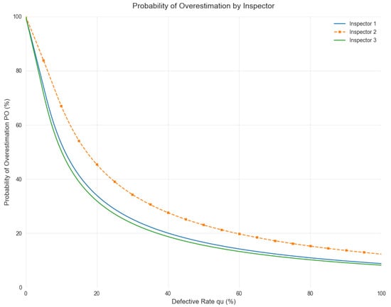
Example 1.
For and the different inspection errors of inspector j for given in Table 3, and for each inspector can be computed by using Proposition 1 and are summarized in the table. If we would like to select the inspector satisfying , then inspector 3 must be selected even though they or an automatic inspection machine is the worst of all in the sense that and .
Table 3.
and for and different inspection errors.
4. Analysis of Model R-II (R, C)
The parameters for Model R-II are provided in Table 4. Suppose that for constant , and A is distributed with . Since is assumed to be , can be obtained as . In the following proposition, the representative shape of as shown in Figure 2 varies depending on the value of , and exists if and only if . Figure 2a shows a typical graph of for without since for . Figure 2b shows a graph of for with . Figure 2c shows a real case of the BLU company in Korea, where , and . Just as shown in the previous example, we are confronted with a similar and unbelievable phenomenon: an imperfect inspector overestimates with if .
Table 4.
Key input and output variables for Model R-II.
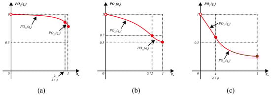
Figure 2.
Three representative graphs of : (a) a typical graph of for without ; (b) a graph of for with ; (c) a typical graph of for with single .
Proposition 2.
For Model R-II (R, C), the following formulas and statements are true:
- 1.
- 2.
- is a strictly decreasing concave function with the supremum and the minimum , and is a strictly decreasing convex function with the maximum and the minimum whereand .
- 3.
- For , does not exist, and an inspector with ρ overestimates with , where can be approximately obtained as 0.7959.For , there exists one and only one and an inspector with ρ overestimates with for , estimates with for and underestimates with for .
Proof.
- 1.
- Equations (5) and (6) can be expressed asEquation (8) can be further reduced towhere .Since the shape of depends upon and , which are dependent each other, Equation (9) can be reduced as follows: For (or equivalently, ), as shown in Figure 3a,.For (or equivalently, ), as shown in Figure 3b,.Even if , the above integral equation holds true since and does not change.
- 2.
- Since from Property A1(1) and from Property A1(2), is a strictly decreasing concave function. Since and from Property A1(3), is a strictly decreasing convex function. Replacing with and using Property A1(4) gives , and we have from Property A1(3).
- 3.
- does not exist if and only if the minimum of exceeds 0.5, i.e., for . Since is a strictly decreasing function of from Property A1(3), solving gives , where can be approximately obtained as 0.7959.For , since and is a strictly decreasing function with , there exists one and only one , which can be obtained by solving for . It follows that , and Proposition 2(3) holds true.
□
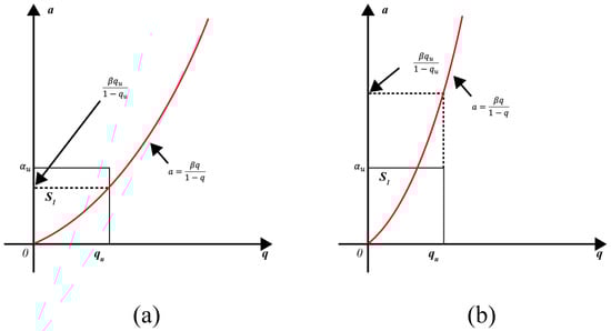
Figure 3.
The shape of region depending on and : (a) for ; (b) for .
Example 2.
For and the different inspection errors of inspector j for given in Table 5, and for each inspector can be computed by using Proposition 2, which are summarized in the table. If we would like to select the inspector satisfying , then, since the of inspector 3 is the closest to 50%, inspector 3 must be selected again even though they/it are/is the worst inspector in the sense that and .
Table 5.
and for and different inspection errors.
5. Analysis of Model R-III (C, R)
The key parameters influencing Model R-III are outlined in Table 6. Supposing that A is constant, and are distributed with . Since is assumed to be , can be obtained as . In the following proposition, (1) the shape of as shown in Figure 4 varies depending on the value of , (2) for , and (3) exists if and only if . Figure 4a shows that the CFB does not exist since exceeds 50% regardless of the value of . Figure 4b shows a graph of for and . Figure 4c shows a real case of a BLU company, where and . It can be observed that an imperfect inspector overestimates with if , overestimates with if , and underestimates with if .
Table 6.
Key input and output variables for Model R-III.
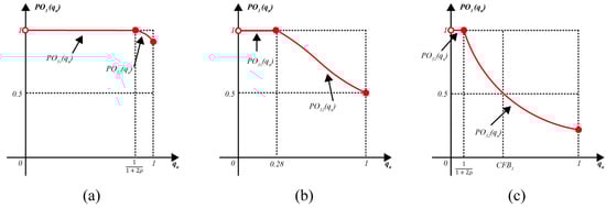
Figure 4.
Three representative graphs of : (a) a typical graph of for without ; (b) a graph of for with ; (c) a typical graph of for with single .
Proposition 3.
For Model R-III (C, R), the following formulas and statements are true:
- 1.
- 2.
- is a strictly decreasing concave function for and a strictly decreasing convex function for , with the maximum and the minimum , where .
- 3.
- For , does not exist, and an inspector with ρ overestimates with , where can be approximately obtained as 1.2564.For , there exists one and only one , which can be obtained by solving,and an inspector with overestimates with for , estimates with for and underestimates with for .
Proof.
- 1.
- Equations (5) and (6) can be expressed asEquation (10) can be further reduced towhere .Since the shape of depends upon and , Equation (11) can be reduced as follows: For , as shown in Figure 5a,For , as shown in Figure 5b,
- 2.
- The first and second derivatives of can be obtained, respectively, asis negative since . By solving , the inflection point of can be obtained at , and it can be proven that is negative for and positive for . The condition that the inflection point exists within 1 becomes . It follows that if , is a strictly decreasing concave function for and a strictly decreasing convex function for . If , is a strictly decreasing concave function with for , where from Property A1(6).
- 3.
- does not exist if and only if the minimum of exceeds 0.5, i.e., for , which gives , where can be approximately obtained as 1.2564. For , since is a strictly decreasing function with , there exists one and only one , which can be obtained by solving or equivalently for . It follows that Proposition 3(3) holds true.
□
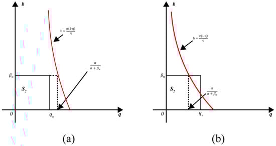
Figure 5.
The shape of the region depending on and : (a) for ; (b) for .
Example 3.
For and the different inspection errors of inspector j for given in Table 7, and for each inspector can be computed by using Proposition 3 and summarized in the table. If we would like to select the inspector satisfying , then since the of inspector 3 is the closest to 50% of all, inspector 3 must be selected again even if and .
Table 7.
and for and different inspection errors.
6. Analysis of Model R-IV (R, R)
Further details on Model R-IV’s input and output variables are provided in Table 8. Suppose that A and B are distributed with and , respectively. Since and , can be obtained as . The computation of requires careful consideration of numerical aspects to ensure accurate results. For , is calculated directly using the formula . Special attention is needed as approaches 0, where the logarithmic term requires careful numerical handling.
Table 8.
Key input and output variables for Model R-IV.
For , the calculation transitions to , which involves the evaluation of multiple terms including . The computation near the transition point is particularly important as it determines the continuity of the probability curve. This transition can be verified by evaluating both formulas at , which should yield identical results.
The existence of is determined by examining . When , exists and can be found by solving . This equation requires careful numerical treatment to ensure accurate results, particularly when is large.
In the following proposition, the representative shape of , which consists of two functions and , varies depending on the value of , and exists if and only if , as shown in Figure 6. Figure 6a shows a typical graph of for , which does not have since for . Figure 6b shows a graph of for , which has . Figure 6c shows a real case of a BLU company, where , . As quality control managers have conjectured, an imperfect inspector overestimates with if .
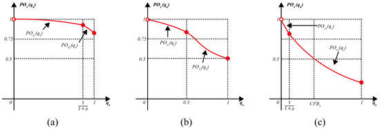
Figure 6.
Three representative graphs of : (a) a typical graph of for without ; (b) a graph of for with ; (c) a typical graph of for with single .
Proposition 4.
For Model R-IV (R, R), can be obtained as
where
Proof.
- 1.
- Equations (5) and (6) can be expressed aswhere , and . From Proposition 7 by Yang and Chang [17], we haveHence, Equation (12) can be further reduced as follows:(1) For (or for , we have(2) For (or for ), we have
□
Proposition 5.
- 1.
- is a strictly decreasing concave function with the minimum and the supremum , where .
- 2.
- is a strictly decreasing function with the maximum and the minimum , where and . In addition, is differentiable at .
- 3.
- does not exist for , and an inspector with overestimates with . For , there exists one and only one , which can be obtained by solving,and an inspector with overestimates with for , estimates with for and underestimates with for .
- 4.
- When , is concave for , and when , is concave for and convex for .
Proof.
- 1.
- For , holds true if and only if from Property A1(7). If , we have from Property A1(4) and from Property A1(8). It follows that , and thus does not exist. If and since is a strictly decreasing function with from Property A1(9), there exists one and only one , which can be obtained by solving or, equivalently for . Hence, an inspector with overestimates with for , estimates with for , and underestimates with for .
- 2.
- Since for and for from Property A3, is concave for and convex for . From Property A2(3), we have if and only if (which equality holds when ) and if and only if , where can be approximately obtained as 0.3646 by solving the equation , which is equivalent to . Hence, statement (4) holds true.
□
Example 4.
For and the different errors of inspector j for given in Table 9, and for each inspector can be computed and are summarized in the table. If we would like to select the inspector satisfying , then the worst inspector 3 must be selected again since the is the closest to 50%. By solving for each inspector, the values of are computed approximately as 11.09%, 17.14%, and 11.6% respectively. Hence, we may conclude that inspector 1 overestimates with if , estimates with if , and underestimates with if . Similar interpretation can be applied to the remaining inspectors. The values of and for each inspector can be obtained as in Table 9 and the curve for each inspector is shown in Figure 7.
Table 9.
and for and different inspection errors.
Figure 7.
Graph of for each inspector.
7. Summary and Concluding Remarks
The major results of Propositions 1– 5 are summarized in Table 10. From this table, the following can be observed:
- 1.
- An imperfect inspector with nonzero inspection errors () has their/its own continuous curve , which depends on two variables and , and is a strictly decreasing function of . It follows that the minimum value of is , and the supremum value of is . From the results of Proposition 1 and 3, we have for Model R-I (C, C) and for Model R-III (C, R). From the results of Proposition 2 and 4, we have for Model R-II (R, C) for Model R-IV (R, R). It follows that . That is, approaches one as approaches zero.
- 2.
- does not exist if and only if . Since is a function of , solving gives the form . From Proposition 1–5, the value of is obtained as one in Model R-I (C, C), in Model R-II (R, C), in Model R-III (C, R), and one in Model R-IV (R, R). It follows that does not exist if and only if , and it means that an inspector with overestimates with more than 50% regardless of . On the other hand, always exists if and only if , and it can be obtained by using the analytical formula given in Model R-I (C, C) or Model R-II (R, C), while it can be obtained by solving the equation given in Model R-III (C, R) or Model R-IV (R, R). When is obtained, an inspector with overestimates with if , estimates with if , and underestimates with if .
Table 10.
Input and output summary of four types of analysis under the assumption of and .
Table 10.
Input and output summary of four types of analysis under the assumption of and .
| Models | Input Parameters | Derived | Output Results |
|---|---|---|---|
| Model R-I (C, C) | Type I error: constant, Type II error: constant, | , | |
| Model R-II (R, C) | Type I error: Type II error: constant, | , | |
| Model R-III (C, R) | Type I error: constant, Type II error: | , | |
| Model R-IV (R, R) | Type I error: Type II error: | , |
Theorem 1.
Assuming an infinite sequence of items with a random DR Q and nonzero inspection errors with and , the following statements are true:
- 1.
- An imperfect inspector with nonzero inspection errors (, ) has their/its own curve with or without .
- 2.
- depends on two variables, and ρ, and can be denoted by , where .
- 3.
- is a decreasing function of with the minimum and maximum , i.e., approaches one as approaches zero.
- 4.
- For , the does not exist, and an inspector with overestimates with , where satisfies .
- 5.
- For , there exists one and only one , which can be obtained by solving , and an inspector with overestimates with for , estimates with for and underestimates with for .
Our theorem implies that the ratio of Type I error to Type II error must go to infinity or the Type I error must become zero. Otherwise, all commercial inspection plans should be, if a given DR is very or extremely low, revised with the concept of the PO for fairness of commercial trades since, from the smaller up to the several hundreds of ppm levels, the larger the DR sold by many sellers, the larger their unfair loss.
These findings have significant implications for industries such as the electronics, automotive, and pharmaceutical industries, where maintaining extremely low defective rates is critical. Overestimation in such contexts can lead to financial inefficiencies, reputational risks, and strained global supply chain relationships. To address these challenges, we recommend incorporating probabilistic models, such as those proposed in this study, into inspection protocols. These models can help establish fairer and more accurate standards in international trade, minimizing unnecessary product rejections. For instance, in semiconductor manufacturing or medical device production, where stringent defect tolerances are essential, our approach can improve inspection accuracy and trade fairness.
Our findings provide valuable insights into the impact of imperfect inspections on overestimation issues. These results can guide revisions to existing inspection schemes by recommending error calibration methods tailored to reduce overestimation biases. For example, the regular recalibration of inspectors’ error rates or the implementation of predictive monitoring systems can improve the reliability of quality assessments. Additionally, our models could complement existing frameworks such as Statistical Process Control (SPC) by incorporating probabilistic error distributions, enabling the more precise control of quality parameters. These practical applications highlight the broader relevance of our theoretical contributions to real-world quality control and inspection strategies.
8. Discussion
This study provides valuable insights into the phenomenon of overestimation during inspection processes. Our theoretical models demonstrate that the probability of overestimation (PO) approaches one as the defect rate (q) approaches zero, regardless of the inspector’s error characteristics. This finding is supported by Monte Carlo simulations, confirming the consistency of PO behavior across various error distributions. Furthermore, the fundamental relationship between and PO is maintained across all tested models, and is identified as a critical factor determining the existence of the critical fraction bound (CFB).
Figure 8 illustrates how PO changes as decreases, highlighting that PO approaches 1 as approaches zero. Further details on the comparative analysis of PO curves can be found in Appendix B. This pattern is consistently observed across different values, supporting the theoretical prediction that overestimation becomes inevitable at extremely low defect rates.
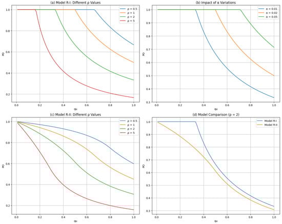
Figure 8.
Analysis of overestimation behavior and model sensitivity: (a) PO variation with different values in Model R-I, showing a consistent pattern as ; (b) impact of Type I error () variations on the PO, demonstrating model robustness; (c) Model R-II behavior under varying values, confirming theoretical predictions; (d) comparison between Models R-I and R-II at , validating model consistency.
Our sensitivity analysis reveals several important implications. The nonlinear relationships between Type I and Type II errors indicate that small changes in parameters can lead to significant variations in the PO within certain critical regions.
Figure 9 further demonstrates these effects by comparing PO under different error distributions. The detailed setup and methodology of the Monte Carlo simulation are presented in Appendix C. The Monte Carlo simulation results confirm that PO can vary significantly depending on the inspector’s accuracy levels and values), reinforcing the need for precise calibration of inspection criteria to minimize overestimation biases.
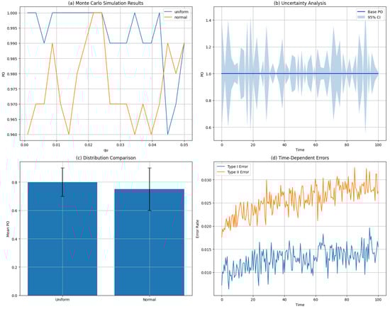
Figure 9.
Validation and practical limitation analysis: (a) Monte Carlo simulation results comparing uniform and normal error distributions; (b) Uncertainty analysis with 95% confidence intervals showing model stability; (c) Comparative analysis of PO under different error distribution assumptions; (d) Time-dependent inspection error patterns demonstrating practical limitations in real inspection environments.
These interaction effects are particularly pronounced when the magnitudes of Type I and Type II errors are comparable. These findings highlight the importance of understanding parameter sensitivity in developing more robust inspection strategies.
Despite the robustness of our theoretical models, there are practical limitations that must be addressed. First, the assumption of independence between Type I and Type II errors may not hold in real-world settings, where correlations can arise due to inspector fatigue or environmental factors. Such correlations could have a significant impact, particularly in automated inspection systems. Second, our models assume time-invariant error rates, which do not account for the temporal variations that may occur in practice. These variations could result in discrepancies between theoretical predictions and actual long-term inspection performance.
The industrial implications of our findings are significant, especially for industries dealing with extremely low defect rates. Conventional inspection protocols may require re-evaluation under these conditions, and optimized inspector selection criteria can be established by considering the relationship between and the CFB. Additionally, the regular recalibration of inspection systems is critical for maintaining accuracy in low-defect-rate environments. From an economic perspective, overestimation in such scenarios can lead to unnecessary costs, underscoring the need for a balanced approach to inspection accuracy and cost management. Investments in enhanced inspection systems are justified for processes where low defect rates are essential.
Future research should focus on extending the current models to incorporate time-dependent error rates and correlated errors. Developing models that integrate measurement system capability limitations would also be beneficial. Validation studies using long-term industrial data are necessary to ensure the practical applicability of our findings. Furthermore, comparative analyses of overestimation patterns across different industries could provide additional insights.
This study contributes to the existing literature by expanding Yang and Chang’s initial research to include random defect rates and enhancing Altay and Baykal-Gürsoy’s inspection scheduling framework. Our work introduces a comprehensive sensitivity analysis, identifies critical parameter regions, and provides practical guidelines for designing more effective inspection systems. While our theoretical framework offers robust insights, careful consideration of its limitations is essential for real-world application. The findings of this study are particularly relevant for industries where maintaining extremely low defect rates is critical, emphasizing the need for a fundamental reassessment of quality control systems.
Funding
The present research was supported by there search fund of Dankook University in 2023.
Data Availability Statement
Not applicable.
Acknowledgments
The author sincerely thanks Moon Hee Yang for his invaluable feedback and guidance on this paper.
Conflicts of Interest
The author declares that there are no conflicts of interest regarding the publication of this paper.
Abbreviations
The following abbreviations are used in this manuscript:
| CF | Critical fraction defective |
| CFB | Critical fraction bound |
| IDR | Imperfect defective rate |
| PO | Probability of overestimation |
| SPC | Statistical Process Control |
| TDR | True defective rate |
| Probability density function | |
| Error rate ratio | |
| Type I error rate | |
| Type II error rate | |
| q | True defective rate (constant) |
| Q | True defective rate (random variable) |
| Distribution of Q | |
| Distribution of Type I errors | |
| Distribution of Type II errors | |
| Critical fraction bound for Model R-I | |
| Critical fraction bound for Model R-II | |
| Critical fraction bound for Model R-III | |
| Critical fraction bound for Model R-IV | |
| Probability of overestimation in R-I | |
| Probability of overestimation in R-II | |
| Probability of overestimation in R-III | |
| Probability of overestimation in R-IV | |
| Expected value of random variable X |
Appendix A. Mathematical Properties and Proofs
This appendix contains detailed mathematical properties and proofs that support the main results presented in this paper. These are included here to maintain the flow of the main text while providing interested readers with the full mathematical details.
Appendix A.1. Properties of Auxiliary Functions
- 1.
- is a strictly increasing function with , where for .
- 2.
- is a strictly increasing function with , where for .
- 3.
- is a strictly decreasing convex function with , where for .
- 4.
- is a strictly decreasing convex function with , where for .
- 5.
- is a strictly decreasing convex function with , where for .
- 6.
- is a strictly increasing function with , where for .
- 7.
- is a strictly decreasing convex function with , where for .
- 8.
- is a strictly decreasing convex function with , where for .
- 9.
- is a strictly decreasing convex function with , where for .
- 10.
- is a strictly decreasing convex function with , where for .
Appendix A.2. Properties Related to Critical Points
- 1.
- , where and .
- 2.
- if and only if (equality holds when ), and if and only if , when is approximately 0.3646, satisfying .
- 3.
- if and only if (equality holds when ), and if and only .
Appendix A.3. Properties of PO42(qu)
- 1.
- is negative for , zero for , and positive for .
- 2.
- If , then is strictly decreasing concave for .
- 3.
- If , then is strictly decreasing concave for , and strictly decreasing concave for .
Appendix B. Comparison of Curves
Comparison of Curves
This section presents a comparative analysis of the curves for the three cases: R-I, R-II, and R-III. The probability of overestimation is analyzed using both constant and random defective rates to demonstrate how the results vary across the models.
The equations representing for each case are as follows:
Here, is the error rate ratio; is the true defective rate threshold.
These equations describe how the probability of overestimation changes with the defective rate model.
Figure A1 shows the curves for each model. The curves highlight the differences in overestimation probabilities across the three cases.
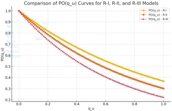
Figure A1.
Comparison of curves for the R-I, R-II, and R-III models. The figure demonstrates how the probability of overestimation changes with the defective rate.
Appendix B.1. Interpretation of Results
- 1.
- Case R-I: The curve is influenced significantly by the parameter and shows a steeper decline as increases.
- 2.
- Case R-II: The curve exhibits a moderate decline, capturing the combined effects of both the error rate ratio and the defective rate threshold.
- 3.
- Case R-III: The curve reflects an exponential relationship and displays the smoothest decline among the three models.
The results demonstrate that the choice of model has a substantial impact on the overestimation probability, particularly when dealing with random defective rates. These findings provide valuable insights into the design of inspection systems under varying defective rate assumptions.
Appendix C. Simulation Study for Random Defective Rate
This appendix provides a detailed simulation study that was conducted to analyze the probability of overestimation (POE) under random defective rates. The results are compared with the findings of Yang and Chang (2014), who considered constant defective rates, to demonstrate the robustness of our extended models.
Appendix C.1. Simulation Setup
The simulation used a uniform distribution for random defective rates to align with the assumptions in this study. The following parameters were applied:
- Random defective rate ∼, with mean defective rates : 0.05, 0.1, 0.2;
- Inspection errors: , ;
- Sample size: 1000;
- Models analyzed: R-I to R-IV.
Appendix C.2. Results and Discussion
The simulation results show distinct POE characteristics for each model. A comparison with the constant defective rate findings from Yang and Chang (2014) highlighted the following:
- 1.
- Low defective rates (): - R-I exhibits a high concentration of POE near 1, consistent with Yang and Chang’s results for constant defective rates. - R-II shows a wider distribution range with bimodal characteristics, indicating sensitivity to random variability. - R-III and R-IV demonstrate more symmetric distributions, reflecting the mixed characteristics of R-I and R-II.
- 2.
- Medium defective rates (): - POE distributions for all models become broader, with R-II showing the most sensitivity to changes in the defective rate. - Compared to Yang and Chang’s results, R-I remains aligned, while the other models provide distinct patterns due to random variability.
- 3.
- High defective rates (): - POE decreases significantly across all models, with lower variability. - R-I and R-IV continue to exhibit higher concentrations near their respective critical fractions.
Appendix C.3. Summary Statistics
Table A1 provides a summary of the mean POE and 95% confidence intervals (CIs) for each model under varying defective rates.
Table A1.
Summary statistics for POE under random defective rates.
Table A1.
Summary statistics for POE under random defective rates.
| Mean Q | Model | Mean POE | 95% CI |
|---|---|---|---|
| 0.05 | R-I | 0.849 | [0.279, 1.000] |
| R-II | 0.248 | [0.000, 0.814] | |
| R-III | 0.381 | [0.171, 1.000] | |
| R-IV | 0.372 | [0.173, 0.833] | |
| 0.10 | R-I | 0.279 | [0.197, 1.000] |
| R-II | 0.004 | [0.000, 0.025] | |
| R-III | 0.158 | [0.103, 0.243] | |
| R-IV | 0.157 | [0.101, 0.252] | |
| 0.20 | R-I | 0.144 | [0.123, 0.172] |
| R-II | 0.000 | [0.000, 0.000] | |
| R-III | 0.068 | [0.054, 0.087] | |
| R-IV | 0.068 | [0.053, 0.087] |
Appendix C.4. Figures
Figure A2 presents the POE distributions for different models under random defective rates, illustrating distinct patterns in overestimation probability. Furthermore, Figure A3 provides a sensitivity analysis, demonstrating how defective rate variability and inspection errors influence the POE.
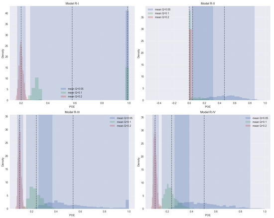
Figure A2.
POE distributions for different models under random defective rates.
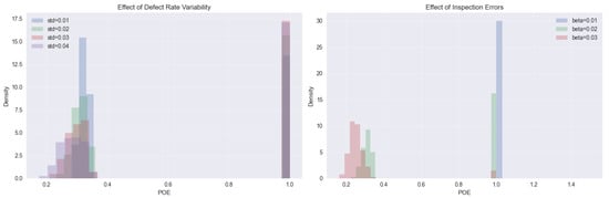
Figure A3.
Sensitivity analysis: effect of defective rate variability and inspection errors on POE.
Appendix C.5. Conclusions
The results confirm the robustness of POE behavior under random defective rates. The patterns observed in R-I align closely with Yang and Chang’s constant defective rate analysis, demonstrating the consistency of our models. Other models provide additional insights into the influence of random variability on the POE.
References
- Collins, R.D.; Kenneth, E.C.; Bennett, G.K. The effects of inspection error on single sampling inspection plans. Int. J. Prod. Res. 1973, 11, 289–298. [Google Scholar] [CrossRef]
- Dorris, A.L.; Foote, B.L. Inspection errors and statistical quality control: A survey. AIIE Trans. 1978, 10, 184–192. [Google Scholar] [CrossRef]
- Raz, T.; Thomas, M.U. A method for sequencing inspection activities subject to errors. IIE Trans. 1983, 15, 12–18. [Google Scholar] [CrossRef]
- Tang, K. Economic Design of Product Specifications for a Complete Inspection Plan. Int. J. Prod. Res. 1987, 26, 203–217. [Google Scholar] [CrossRef]
- Lee, H.L. On the Optimality of a Simplified Multi characteristic Component Inspection Model. IIE Trans. 1988, 20, 392–398. [Google Scholar] [CrossRef]
- Duffuaa, S.O.; Khan, M. A general repeat inspection plan for dependent multi characteristic critical components. Eur. J. Oper. Res. 2008, 191, 374–385. [Google Scholar] [CrossRef]
- Yang, M.; Cho, J.H. Minimization of Inspection and Rework Cost in a BLU factory Considering Imperfect inspection. Int. J. Prod. Res. 2013, 52, 384–396. [Google Scholar] [CrossRef]
- Sylla, C.; Drury, C.G. Signal detection for human error correction in quality control. Comput. Ind. 1995, 26, 147–159. [Google Scholar] [CrossRef]
- Burk, R.J.; Davis, R.D.; Kaminsky, F.C.; Roberts, A.E.P. The effect of inspector errors on the true fraction nonconforming: An industrial experiment. Qual. Eng. 1995, 7, 543–550. [Google Scholar] [CrossRef]
- Yang, M. A Design and Case Study of a K-Stage BLU Inspection System for Achieving a Target Defective Rate. Int. J. Manag. Sci. 2007, 13, 141–157. [Google Scholar]
- Campari, A.; Ustolin, F.; Alvaro, A.; Paltrinieri, N. Inspection of hydrogen transport equipment: A data-driven approach to predict fatigue degradation. Reliab. Eng. Syst. Saf. 2024, 240, 109071. [Google Scholar] [CrossRef]
- Altay, N.; Baykal-Gürsoy, M. Imperfect rail-track inspection scheduling with zero-inflated miss rates. Reliab. Eng. Syst. Saf. 2022, 138, 103608. [Google Scholar]
- Manna, A.K.; Dey, J.K.; Mondal, S.K. Effect of inspection errors on imperfect production inventory model with warranty and price discount dependent demand rate. RAIRO-Oper. Res. 2020, 54, 1189–1213. [Google Scholar] [CrossRef]
- Mokhtari, H.; Asadkhani, J. Extended economic production quantity models with preventive maintenance . Int. J. Invent. Res. 2020, 27, 3253–3264. [Google Scholar]
- Song, Y.; Li, F.; Wang, Z.; Zhang, B. Uncertainty quantification of data-driven quality prediction model for realizing active sampling inspection of mechanical properties in steel production. Int. J. Adv. Manuf. Technol. 2024, 121, 451–460. [Google Scholar] [CrossRef]
- Ashebir, D.A.; Hendlmeier, A.; Dunn, M.; Arablouei, R. Defects in material extrusion additive manufacturing of fiber-reinforced thermoplastic composites: A review of challenges and advanced non-destructive testing methods. Polymers 2024, 16, 2986. [Google Scholar] [CrossRef]
- Yang, M.H.; Chang, K. A Study on Overestimating a Given Fraction Defective by an Imperfect Inspector. Math. Probl. Eng. 2014, 2014, 619639. [Google Scholar] [CrossRef]
Disclaimer/Publisher’s Note: The statements, opinions and data contained in all publications are solely those of the individual author(s) and contributor(s) and not of MDPI and/or the editor(s). MDPI and/or the editor(s) disclaim responsibility for any injury to people or property resulting from any ideas, methods, instructions or products referred to in the content. |
© 2025 by the author. Licensee MDPI, Basel, Switzerland. This article is an open access article distributed under the terms and conditions of the Creative Commons Attribution (CC BY) license (https://creativecommons.org/licenses/by/4.0/).