Bezier Curves and Surfaces with the Generalized α-Bernstein Operator

Abstract

In the field of Computer-Aided Geometric Design (CAGD), a proper model can be achieved depending on certain characteristics of the predefined blending basis functions. The presence of these characteristics ensures the geometric properties necessary for a decent design. The objective of this study, therefore, is to examine the generalized $\alpha$-Bernstein operator in the context of its potential classification as a novel blending type basis for the construction of Bézier-like curves and surfaces. First, a recursive definition of this basis is provided, along with its unique representation in terms of that for the classical Bernstein operator. Next, following these representations, the characteristics of the basis are discussed, and one shape parameter for $\alpha$-Bezier curves is defined. In addition, by utilizing the recursive definition of the basis, a de Casteljau-like algorithm is provided such that a subdivision schema can be applied to the construction of the new $\alpha$-Bezier curves. The parametric continuity constraints for $C^0$, $C^1$, and $C^2$ are also established to join two $\alpha$-Bezier curves. Finally, a set of cross-sectional engineering surfaces is designed to indicate that the generalized $\alpha$-Bernstein operator, as a basis, is efficient and easy to implement for forming shape-adjustable designs.

1. Introduction

In CAGD, free-form curves are essential in various scientific and engineering applications, such as designing car bodies, ship hulls, and aircraft, among other things [1,2]. In order to create such forms, a particularly useful method proposed by the French mathematician Pierre Etienne Bezier in the 1960s plays a crucial role due to its efficiency and practical applicability. This method relies on a blending process for the given control points where the blending functions are well-known Bernstein polynomials [2]. As a consequence of this method, the resulting parametric relation corresponds to a simple free-form curve widely known as a Bezier curve. This modeling technique, particularly concerning the control points, enables the shape of the curves to be flexibly adapted to the designer’s demands. However, these curves are limited in representing transcendental curves due to the polynomial form of the Bernstein operator. Another limitation is the dependency of the curve’s shape on the control points. To address these limitations, new adjustable Bezier curves with modified Bernstein polynomials possessing multiple shape parameters have been introduced [3,4,5,6,7,8,9,10]. Moreover, to represent more types of curves using the Bezier method, numerous studies have been devoted to defining new blending type bases with trigonometric, hyperbolic, exponential, and logarithmic functions [11,12,13,14,15,16,17,18,19,20,21,22]. Therefore, it becomes a very important practice for researchers to define a new basis and then construct new more effective and adjustable curves.

To account for a new basis, the theory of Chebyshev spaces is widely used [12,15,23,24]. The probabilistic distribution functions are also considered new bases [2,25,26,27,28] since the Bernstein polynomials are equivalent to a binomial distribution function. In addition, researchers have also derived mutual benefits from the interdisciplinary relation between the approximation theory and geometric design. Cai et al. [29], for example, studied the approximation properties of the modified Bernstein operator which was originally defined by Ye et al. in [6] for the purpose of constructing Bezier-like curves. Similarly, a novel generalization of the Bernstein operator introduced previously in [10] was reconsidered in [30] as a new operator for approximation purposes. However, not all of the functions used for approximation purposes are suitable for an effective geometric design. They must exhibit specific characteristics, as outlined in

Table 1. The characteristics which the basis functions should posses for a proper design within the scope of CAGD [26].

	Free-Form Geometric Design		Blending (/Basis) Functions
1	well-defined	⇔	$\sum f_k^n\left(t\right)=1$
2	convex hull	⇔	$f_k^n\left(t\right)\ge 0$
3	smooth	⇔	$f_k^n\left(t\right)$ differentiable
4	interpolate end-points	⇔	$f_0^n\left(0\right)=1=f_n^n\left(1\right)$ ve $f_{1\le i\le n-1}^n\left(0\right)=0=f_{1\le i\le n-1}^n\left(1\right)$
5	surface design	⇔	the product $f_i^n\left(u\right)·f_j^m\left(v\right)$ possesses 1, 2, 3, and 4
6	symmetry	⇔	$f_k^n\left(t\right)=f_{n-k}^n(1-t)$
7	construction algorithm	⇐	$f_k^n\left(t\right)=(1-t)f_k^{n-1}\left(t\right)+t{f}_{k-1}^{n-1}\left(t\right)$
8	non-degenerate	⇔	$f_k^n\left(t\right)$ linearly independent

. Therefore, in this study, the discussion is focused on the generalized $\alpha$-Bernstein operator, which was previously examined in terms of its approximation properties by Chen et al. [31]. For further clarification, this paper explores the characterizations of the generalized $\alpha$-Bernstein operator in the realm of the creation of Bezier-like curves and surfaces.

The structure of this paper is as follows: Section 2 recalls the basic definitions for the classic Bezier curves and surfaces, as well as the generalized $\alpha$-Bernstein operator. In Section 3, the main results of this paper are given by providing some other unique representations of the generalized $\alpha$-Bernstein operator. Following these representations, the characteristics of the new operator are discussed as well. Further, the definition of the new $\alpha$-Bezier curve and its geometric properties are given in this section, along with the parametric continuity conditions. Finally, a set of engineering surfaces and the tensor product $\alpha$-Bezier surface patch are built and figured to indicate the eligibility and applicability of the basis. In the last section of the research, our final remarks are proposed in a concise manner.

2. Preliminaries

In this section, we will recall some basic concepts to which we will refer through out this paper.

Definition 1. 

An $nth$-degree classical Bezier curve with given $n+1$ control points $P_k\in {\mathbb{R}}^2(/{\mathbb{R}}^3),k=0,1,\dots ,n$, is defined as follows:

$${}_{\mathcal{C}}\mathcal{B}\left(s\right)=\sum _{k=0}^n{b}_k^n\left(s\right)P_k$$

(1)

where ${\displaystyle b_k^n\left(s\right)=\left(\genfrac{}{}{0pt}{}{n}{k}\right){(1-s)}^{n-k}{s}^k,s\in [0,1]}$ is the classic Bernstein operator, and ${\displaystyle \left(\genfrac{}{}{0pt}{}{n}{k}\right)=\frac{n!}{(n-k)!k!}}$ is the well-known binomial coefficient [2].

Definition 2. 

A tensor product Bezier surface patch of degree $(n+1,m+1)$ with given control points $P_{ij}\in {\mathbb{R}}^2(/{\mathbb{R}}^3),(i=0,1,\dots ,n),(j=0,1,\dots ,m)$ is defined by the following:

$${}_{\mathcal{S}}\mathcal{B}\left(u,v\right)=\sum _{i=0}^n\sum _{j=0}^m{b}_i^n\left(u\right)b_j^m\left(v\right)P_{ij}$$

(2)

where for $u,v\in [0,1]$, $b_i^n\left(u\right)$ and $b_j^m\left(v\right)$ are the classic Bernstein operators of degree n and m, respectively.

Definition 3. 

Given $p_0^1(s;\alpha )=1-s,p_1^1(s;\alpha )=s$, the generalized $n^{th}$-degree α-Bernstein operator is defined as follows:

$$p_k^n(s;\alpha )=\left(\left({\displaystyle \genfrac{}{}{0pt}{}{n-2}{k}}\right)\left(1-\alpha \right)s+\left({\displaystyle \genfrac{}{}{0pt}{}{n-2}{k-2}}\right)\left(1-\alpha \right)\left(1-s\right)+\left({\displaystyle \genfrac{}{}{0pt}{}{n}{k}}\right)\alpha s\left(1-s\right)\right)s^{k-1}{\left(1-s\right)}^{n-1-k}$$

(3)

where $s\in \left[0,1\right],n\ge 2$ and $k=0,1,\dots ,n$, [31].

3. Main Results

The classic Bezier curves and surfaces have unique properties which are useful and essential for geometric designs. Such properties are acquired by them inheriting the attributes of the classic Bernstein operator which can be found in [32]. Therefore, in this section, the similar attributes of the generalized $\alpha$-Bernstein operator are discussed. In order to define these characteristics, a recursive definition of the generalized $\alpha$-Bernstein operator is given. Then, a unique relation between the classic Bernstein and the generalized $\alpha$-Bernstein operator is provided. By following these definitions and representations, we examine the characterizations of the generalized $\alpha$-Bernstein operator.

Proposition 1. 

Let $\alpha \in [0,1]$, and for $0\le s\le 1$, the functions

$$\left\{\begin{array}{cc}\hfill p_0^2(s;\alpha )& =(1-s)(1-\alpha s),\hfill \\ \hfill p_1^2(s;\alpha )& =2s(1-s)\alpha ,\hfill \\ \hfill p_2^2(s;\alpha )& =s\left(1-a\left(1-s\right)\right)\hfill \end{array}\right.$$

(4)

are called the α-Bernstein polynomials of order 2. For $n\ge 2$, the generalized α-Bernstein polynomials can be recursively defined by the following:

$$p_k^n\left(s;\alpha \right)=\left(1-s\right)p_k^{n-1}\left(s;\alpha \right)+s{p}_{k-1}^{n-1}\left(s;\alpha \right)$$

(5)

where $p_i^m\left(s;\alpha \right)=0$, when $i=-1$ or $i>m$.

Proposition 2. 

The generalized α-Bernstein operator can explicitly be expressed by the classical Bernstein operator as

$$p_k^n\left(s;\alpha \right)=\left(1-\alpha \right)\left[b_{k-1}^{n-1}\left(s\right)-b_{k-1}^{n-2}\left(s\right)+b_k^{n-1}\left(s\right)\right]+\alpha b_k^n\left(s\right).$$

(6)

Proof. 

Let us re-express the generalized $\alpha$-Bernstein operator by expanding the relation (3) as

$$p_k^n\left(s,\alpha \right){=}_1{l}_k^n\left(s,\alpha \right){+}_2{l}_k^n\left(s,\alpha \right){+}_3{l}_k^n\left(s,\alpha \right),$$

where

$$\begin{array}{cc}\hfill {}_{1}l_k^n\left(s,\alpha \right)& =\left(1-\alpha \right)\left({\displaystyle \genfrac{}{}{0pt}{}{n-2}{k}}\right)s^k{\left(1-s\right)}^{n-k-1},\hfill \\ \hfill {}_{2}l_k^n\left(s,\alpha \right)& =\left(1-\alpha \right)\left({\displaystyle \genfrac{}{}{0pt}{}{n-2}{k-2}}\right)s^{k-1}{\left(1-s\right)}^{n-k},\hfill \\ \hfill {}_{3}l_k^n\left(s,\alpha \right)& =\alpha \left({\displaystyle \genfrac{}{}{0pt}{}{n}{k}}\right)s^k{\left(1-s\right)}^{n-k}.\hfill \end{array}$$

We note that if $k=n-1$ or $k=n$, then ${}_{1}l_k^n\left(s,\alpha \right)=0$. Similarly, if $k=0$ or $k=1$, then ${}_{2}l_k^n\left(s,\alpha \right)=0$. Thus, we may rewrite the generalized $\alpha$-Bernstein operator in terms of the classic Bernstein operator in the following way:

$$p_k^n\left(s,\alpha \right)=\left(1-\alpha \right)\left[\left(1-s\right)b_k^{n-2}\left(s\right)+s{b}_{k-2}^{n-2}\left(s\right)\right]+\alpha b_k^n\left(s\right)$$

(7)

Moreover, by utilizing the following two recursive relations of the classic Bernstein polynomials

$$\begin{array}{c}{b}_{k-1}^{n-1}\left(s\right)=(1-s)b_{k-1}^{n-2}\left(s\right)+s{b}_{k-2}^{n-2}\left(s\right)\hfill \\ b_k^{n-1}\left(s\right)=(1-s)b_k^{n-2}\left(s\right)+s{b}_{k-1}^{n-2}\left(s\right)\hfill \end{array},$$

and by adding them together and substituting them into (7), we complete the proof. □

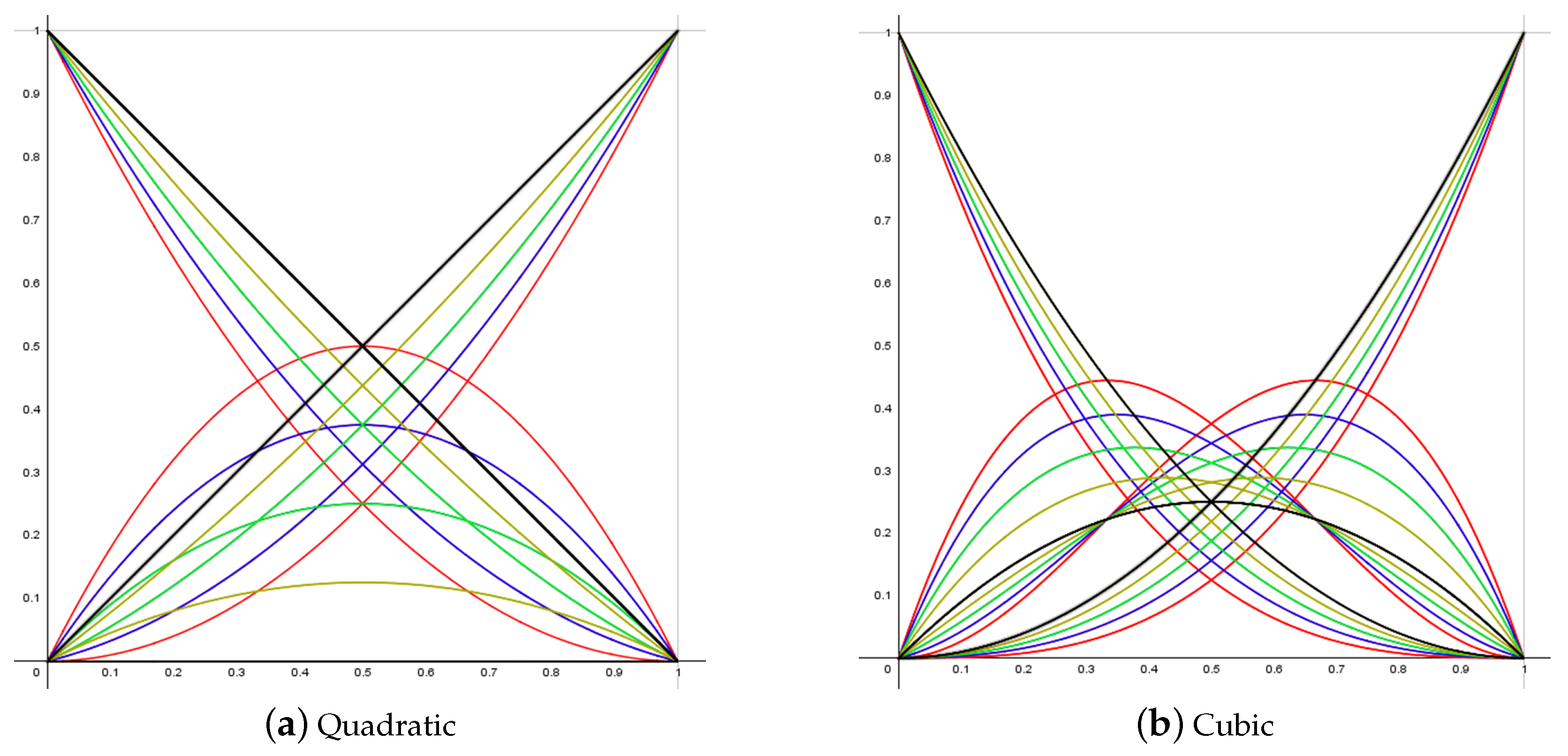
3.1. The Properties of the Generalized $\alpha$-Bernstein Operator

The following properties exist for the generalized $\alpha$-Bernstein operator $p_k^n\left(s;\alpha \right)$ for $s,\alpha \in [0,1]$ where $n\ge 2$.

• Degeneracy: For $\alpha =1$, the generalized $\alpha$-Bernstein operator is reduced into the classic Bernstein operator.
  The result follows from relation (6) in Proposition 2.
• Non-negativity: The generalized $\alpha$-Bernstein polynomials are non-negative for $s,\alpha \in [0,1]$.
  Since the classic Bernstein operator is non-negative, that is, $b_k^n\left(s\right)\ge 0,$ for $0\le s\le 1$, [32] and $\left(1-\alpha \right)\ge 0$ and $\alpha \ge 0$ for $\alpha \in [0,1]$, it is clear from (6) that $p_k^n\left(s;\alpha \right)\ge 0$.
• Partition of unity: The generalized $\alpha$-Bernstein operator is normalized, that is, ${\displaystyle \sum _{k=0}^n}{p}_k^n(s;\alpha )=1$.
  By utilizing relation (6), we have

  $$\sum _{k=0}^n{p}_k^n(s;\alpha )=\sum _{k=0}^n\left(1-\alpha \right)\left[b_{k-1}^{n-1}\left(s\right)-b_{k-1}^{n-2}\left(s\right)+b_k^{n-1}\left(s\right)\right]+\alpha b_k^n\left(s\right).$$
  Further, by making the appropriate change in indices as $k_1=k-1$ and due to the classic Bernstein operator summing to 1, we obtain

  $$\begin{array}{cc}\hfill \sum _{k=0}^n{p}_k^n(s;\alpha )& =\left(1-\alpha \right)\left[\sum _{k_1=0}^{n-2}{b}_{k_1}^{n-2}\left(s\right)-\sum _{k_1=0}^{n-2}{b}_{k_1}^{n-2}\left(s\right)+\sum _{k=0}^{n-1}{b}_k^{n-1}\left(s\right)\right]+\alpha \sum _{k=0}^n{b}_k^n\left(s\right)\hfill \\ \hfill & =\left(1-\alpha \right)·[1-1+1]+\alpha ·1=1.\hfill \end{array}$$
• Linear independence: The generalized $\alpha$-Bernstein polynomials are linearly independent, that is, ${\displaystyle \sum _{k=0}^n}{c}_k{p}_k^n(s;\alpha )=0\iff c_k=0$, for $k=0,1,\dots ,n$.
  Proof. 

  We establish this property through induction on n. The sufficient part of the result is clear. The necessary part can be carried out as follows. For $n=2$, let us consider the linear combination ${\displaystyle \sum _{k=0}^2}{c}_k{p}_k^2(s;\alpha )=0$, where $c_k\in R,k=0,1,2$. By using (6) and making some algebraic manipulations, we have

  $$\left(1-\alpha \right)\left(\left(c_0+c_1\right)b_0^1\left(s\right)+\left(c_1+c_2\right)b_1^1\left(s\right)-c_1\right)+\alpha \left(c_0{b}_0^2\left(s\right)+c_1{b}_1^2\left(s\right)+c_2{b}_2^2\left(s\right)\right)=0.$$

  As the classic Bernstein polynomials are linearly independent (see [32]), we obtain the following system of equations:

  $$\left\{\begin{array}{ccccc}\alpha c_0=0,\hfill & \alpha c_1=0,\hfill & \alpha c_2=0\hfill & & \left(i\right)\hfill \\ \left(1-\alpha \right)c_1=0\hfill & & & & \left(ii\right)\hfill \\ \left(1-\alpha \right)\left(c_0+c_1\right)=0,\hfill & \left(1-\alpha \right)\left(c_1+c_2\right)=0\hfill & & & \left(iii\right)\hfill \end{array}\right.$$

  Clearly, if $\alpha \ne 0$, then from relations in $\left(i\right)$, $c_k=0,k=0,1,2$. If $\alpha =0$, then from the relation given in $\left(ii\right)$, $c_1=0$. This results as a consequence in $c_0=c_2=0$ upon the consideration of the two equations in $\left(iii\right)$. Now, assume that the linear independence holds for $n=l$. Thus, for $n=l+1$, we consider

  $$\sum _{k=0}^{l+1}{c}_k{p}_k^{l+1}(s;\alpha )=0k=0,1,\dots ,l+1.$$

  By recalling the recursive definition of the generalized $\alpha$-Bernstein operator given in (5), we re-express the last equation as follows:

  $$\begin{array}{cc}\hfill \sum _{k=0}^{l+1}{c}_k{p}_k^{l+1}(s;\alpha )& =\sum _{k=0}^{l+1}{c}_k\left[\left(1-s\right)p_k^l\left(s;\alpha \right)+s{p}_{k-1}^l\left(s;\alpha \right)\right]\hfill \\ & =\left(1-s\right)\sum _{k=0}^{l+1}{c}_k{p}_k^l\left(s;\alpha \right)+s\sum _{k=0}^{l+1}{c}_k{p}_{k-1}^l\left(s;\alpha \right)=0.\hfill \end{array}$$

  In view of the fact that the parameter s is an arbitrary real number in the interval $[0,1]$, we conclude that

  $$\left\{\sum _{k=0}^{l+1}{c}_k{p}_k^l\left(s;\alpha \right)=0,\sum _{k=0}^{l+1}{c}_k{p}_{k-1}^l\left(s;\alpha \right)=0.\right.$$

  By recalling that $p_i^m\left(s;\alpha \right)=0$ when $i=-1$ or $i>m$ and by considering our inductive hypothesis, that is, $c_k=0,k=0,1,\dots l$, we clearly deduce that $c_k=0,$ for $k=0,1,\dots l+1$, which completes the proof. □
• Symmetry: The generalized $\alpha$-Bernstein operator is symmetric such that $p_k^n\left(1-s;\alpha \right)=p_{n-k}^n\left(s;\alpha \right).$
  Proof. 

  We prove this through induction on n. For $n=2$, the property is easy to validate from relation (4). Further, assume that it holds for $n=l$. Next, for $n=l+1$, and from (5), we first write

  $$p_k^{l+1}\left(1-s;\alpha \right)=s{p}_k^l\left(1-s;\alpha \right)+\left(1-s\right)p_{k-1}^l\left(1-s;\alpha \right)$$

  with the replacement of s with $1-s$. Furthermore, by utilizing our inductive hypothesis and using the recursive expression (5), we re-express the right-hand side of the above relation as follows:

  $$\begin{array}{cc}\hfill p_k^{l+1}\left(1-s;\alpha \right)& =s{p}_{l-k}^l\left(s;\alpha \right)+\left(1-s\right)p_{l+1-k}^l\left(s;\alpha \right)\hfill \\ & =p_{l+1-k}^{l+1}\left(s;\alpha \right),\hfill \end{array}$$

  which completes the proof. □
• End-points: At the end-points, the generalized $\alpha$-Bernstein operator has the same properties as those of the classic Bernstein operator, that is, for $k=0,\dots ,n$

  $$p_k^n\left(0;\alpha \right)=\left\{\begin{array}{ccc}1\hfill & :\hfill & k=0\hfill \\ 0\hfill & :\hfill & k\ne 0\hfill \end{array}\right.,p_k^n\left(1;\alpha \right)=\left\{\begin{array}{ccc}1\hfill & :\hfill & k=n\hfill \\ 0\hfill & :\hfill & k\ne n\hfill \end{array}\right..$$
  Proof. 

  The proof is induced on n. For $n=2$, it is clear that the property holds from (4). Now, assume that the property holds for $n=l$. Then, for $n=l+1$ and by considering (5), we have $p_k^{l+1}\left(0;\alpha \right)=p_k^l\left(0;\alpha \right)$ where $s=0$. From the inductive hypothesis, we obtain the following:

  $$p_k^{l+1}\left(0;\alpha \right)=p_k^l\left(0;\alpha \right)=\left\{\begin{array}{ccc}1\hfill & :\hfill & k=0\hfill \\ 0\hfill & :\hfill & k\ne 0\hfill \end{array}\right..$$

  Similarly, for $s=1$ and from (5), we obtain $p_k^{l+1}\left(1;\alpha \right)=p_{k-1}^l\left(1;\alpha \right)$. Further, from the inductive hypothesis, we can complete the proof with the following:

  $$p_{k-1}^l\left(1;\alpha \right)=\left\{\begin{array}{ccc}1\hfill & :\hfill & k-1=l\hfill \\ 0\hfill & :\hfill & k-1\ne l\hfill \end{array}\right.\Rightarrow p_k^{l+1}\left(1;\alpha \right)=\left\{\begin{array}{ccc}1\hfill & :\hfill & k=l+1\hfill \\ 0\hfill & :\hfill & k\ne l+1\hfill \end{array}\right.·$$

  □
• Derivatives at the corner points: The first derivatives of the generalized $\alpha$-Bernstein polynomials at the end-points are given as follows:

  $${\displaystyle \frac{\partial p_k^n\left(s;\alpha \right)}{\partial s}}{|}_{s=0}=\left\{\begin{array}{ccc}1-\left(\alpha +n\right)\hfill & :\hfill & k=0\hfill \\ n-2\left(1-\alpha \right)\hfill & :\hfill & k=1\hfill \\ 1-\alpha \hfill & :\hfill & k=2\hfill \\ 0\hfill & :\hfill & \mathrm{other}\hfill \end{array}\right.,$$

  and

  $${\displaystyle \frac{\partial p_k^n\left(s;\alpha \right)}{\partial s}}{|}_{s=1}=\left\{\begin{array}{ccc}-1+\left(\alpha +n\right)\hfill & :\hfill & k=n\hfill \\ -n+2\left(1-\alpha \right)\hfill & :\hfill & k=n-1\hfill \\ -\left(1-\alpha \right)\hfill & :\hfill & k=n-2\hfill \\ 0\hfill & :\hfill & \mathrm{other}\hfill \end{array}\right..$$
  Proof. 

  Similar to the above, the proof is induced on n. By taking the first-order derivative of (4), we have

  $$\left\{\begin{array}{cc}\hfill p_0^2{(s;\alpha )}^{\prime }& =-1-\alpha +2\alpha s,\hfill \\ \hfill p_1^2{(s;\alpha )}^{\prime }& =2\alpha \left(1-2s\right),\hfill \\ \hfill p_2^2{(s;\alpha )}^{\prime }& =1-\alpha +2\alpha s.\hfill \end{array}\right.$$

  For $n=2$, it is clear to see that the given expressions hold when they are evaluated at $s=0$ and $s=1$, respectively. Now, let us suppose that the expressions hold for $n=l$. Then, for $n=l+1$ and from (5), we have

  $$p_k^{l+1}\left(s;\alpha \right)=\left(1-s\right)p_k^l\left(s;\alpha \right)+s{p}_{k-1}^l\left(s;\alpha \right).$$

  By taking the derivative of this expression and evaluating it at $s=0$, we have

  $$p_k^{l+1}{\left(0;\alpha \right)}^{\prime }=-p_k^l\left(0;\alpha \right)+p_k^l{\left(0;\alpha \right)}^{\prime }+p_{k-1}^l\left(0;\alpha \right).$$

  Next, by considering the inductive hypothesis and the end-point properties, we can provide the following conclusions:

  if $k=0$, then $\left\{\begin{array}{cccc}{p}_0^{l+1}{\left(0;\alpha \right)}^{\prime }\hfill & =-p_0^l\left(0;\alpha \right)\hfill & +\hfill & p_0^l{\left(0;\alpha \right)}^{\prime }\hfill \\ & =-1\hfill & +\hfill & 1-\left(\alpha +n\right)=1-\left(\alpha +n+1\right)\hfill \end{array}\right.$,

  if $k=1$, then $\left\{\begin{array}{ccccc}{p}_1^{l+1}{\left(0;\alpha \right)}^{\prime }\hfill & =p_1^l\left({0;\alpha }^{\prime }\right)\hfill & +\hfill & p_0^l{\left(0;\alpha \right)}^{\prime }\hfill & \\ & =n-2\left(1-\alpha \right)\hfill & +\hfill & 1\hfill & =n+1-2\left(1-\alpha \right)\hfill \end{array}\right.$,

  and finally

  if $k=2$, then $\left\{\begin{array}{cc}{p}_2^{l+1}{\left(0;\alpha \right)}^{\prime }\hfill & =p_2^l{\left(0;\alpha \right)}^{\prime }\hfill \\ & =\left(1-\alpha \right)\hfill \end{array}\right.$.

  By following similar steps for $s=1$, the proof is completed. □
• Second-order derivatives: The second-order derivatives of the generalized $\alpha$-Bernstein polynomials at the end-points are given as follows:

  $$\begin{array}{cc}\hfill {\displaystyle \frac{{\partial }^2{p}_k^n\left(s;\alpha \right)}{\partial s^2}}{|}_{s=0}=& \left\{\begin{array}{ccc}\left(n-1\right)\left(n-2\left(1-\alpha \right)\right)\hfill & :\hfill & k=0\hfill \\ 2\left(n\left(1-n\right)+\left(3n-4\right)\left(1-\alpha \right)\right)\hfill & :\hfill & k=1\hfill \\ n\left(n-1\right)-2\left(3n-5\right)\left(1-\alpha \right)\hfill & :\hfill & k=2\hfill \\ 2\left(n-2\right)\left(1-\alpha \right)\hfill & :\hfill & k=3\hfill \\ 0\hfill & :\hfill & \mathrm{other}\hfill \end{array}\right.,\hfill \\ \hfill \mathrm{and}& \\ \hfill {\displaystyle \frac{{\partial }^2{p}_k^n\left(s;\alpha \right)}{\partial s^2}}{|}_{s=1}=& \left\{\begin{array}{ccc}\left(n-1\right)\left(n-2\left(1-\alpha \right)\right)\hfill & :\hfill & k=n\hfill \\ 2\left(n\left(1-n\right)+\left(3n-4\right)\left(1-\alpha \right)\right)\hfill & :\hfill & k=n-1\hfill \\ n\left(n-1\right)-2\left(3n-5\right)\left(1-\alpha \right)\hfill & :\hfill & k=n-2\hfill \\ 2\left(n-2\right)\left(1-\alpha \right)\hfill & :\hfill & k=n-3\hfill \\ 0\hfill & :\hfill & \mathrm{other}\hfill \end{array}\right..\hfill \end{array}$$

  (8)
  Proof. 

  Parallel to the above, the proof can be achieved by using induction on n where the initial step starts with $n=3$. □

The following, Figure 1, illustrates the generalized $\alpha$-Bernstein polynomials of order two and three with different values for the parameter $\alpha$.

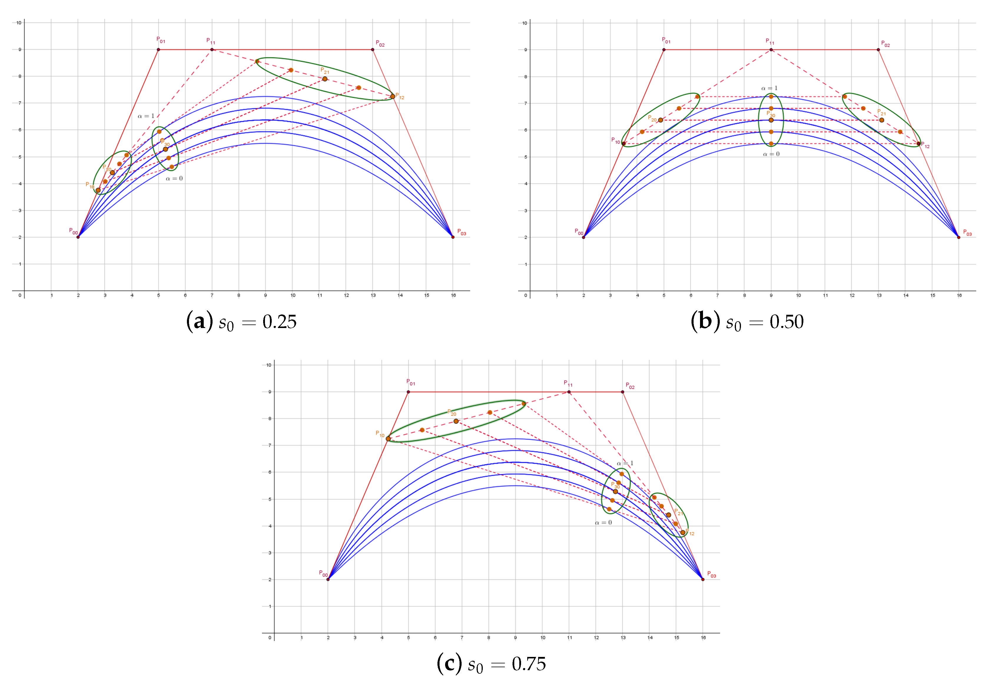
3.2. The Construction of $\alpha$-Bezier Curves

In this section, the $\alpha$-Bezier curves are defined by incorporating the basis of the $\alpha$-Bernstein operator, and the characterizations of the curves are examined in parallel with the properties of the basis. A de Casteljau-like subdivision algorithm is also given. The parametric continuity conditions up to the second degree are obtained for two adjacent $\alpha$-Bezier curves as well.

Definition 4. 

For $\alpha \in [0,1]$, the novel one shape parameter of an α-Bezier curve with given $n+1$ control points $P_k\in {\mathbb{R}}^2(/{\mathbb{R}}^3),k=0,1,\dots ,n$ is defined as

$$\mathcal{B}\left(s;\alpha \right)=\sum _{k=0}^n{p}_k^n\left(s;\alpha \right)P_k,s\in [0,1]$$

(9)

where $n\ge 2$, and $p_k^n(s;\alpha )$ is the generalized α-Bernstein operator, as defined in (3).

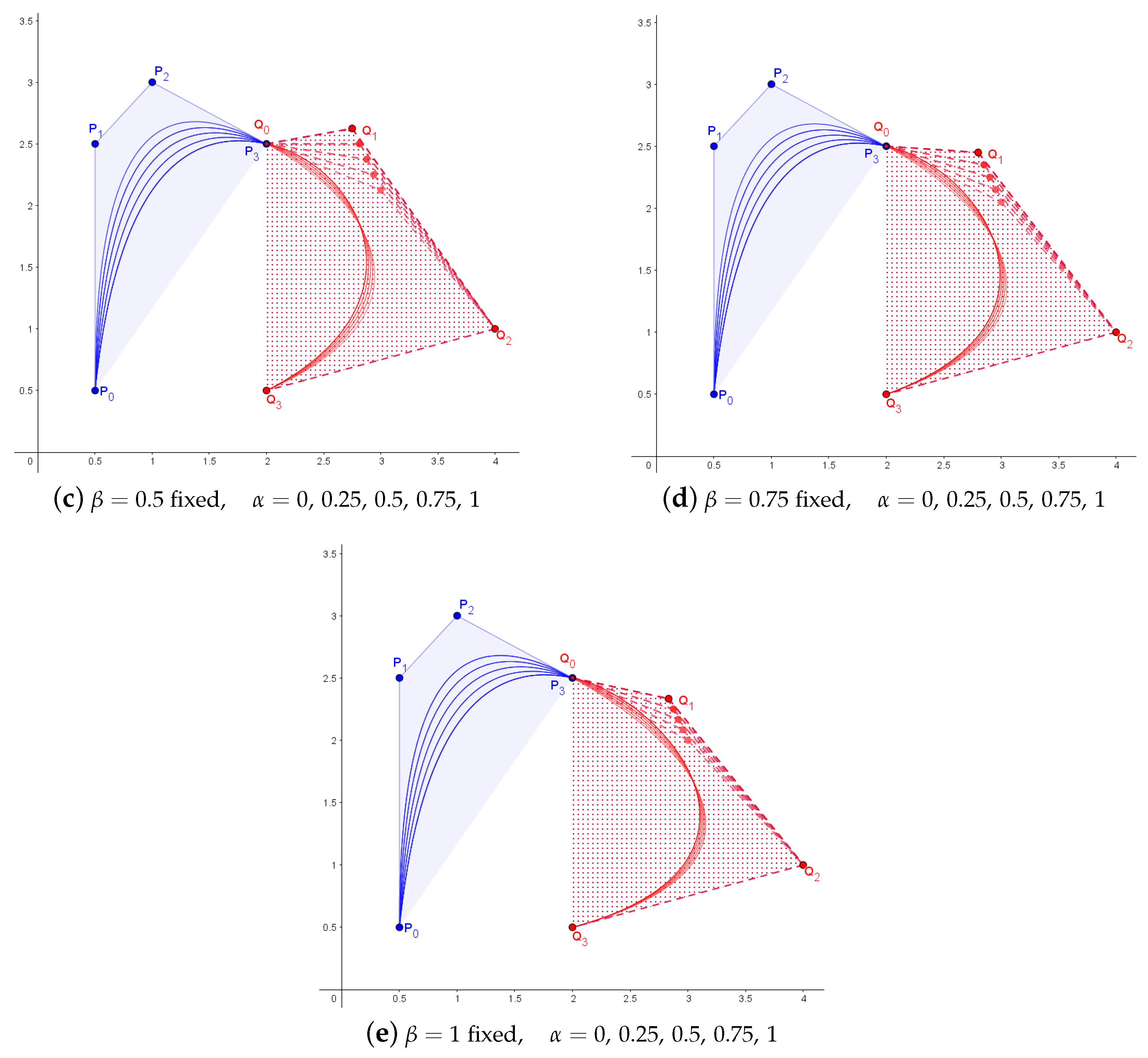
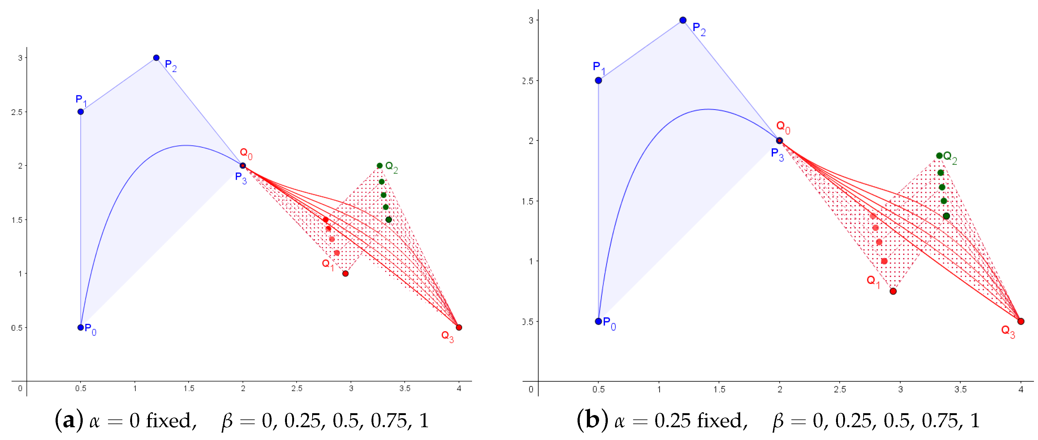
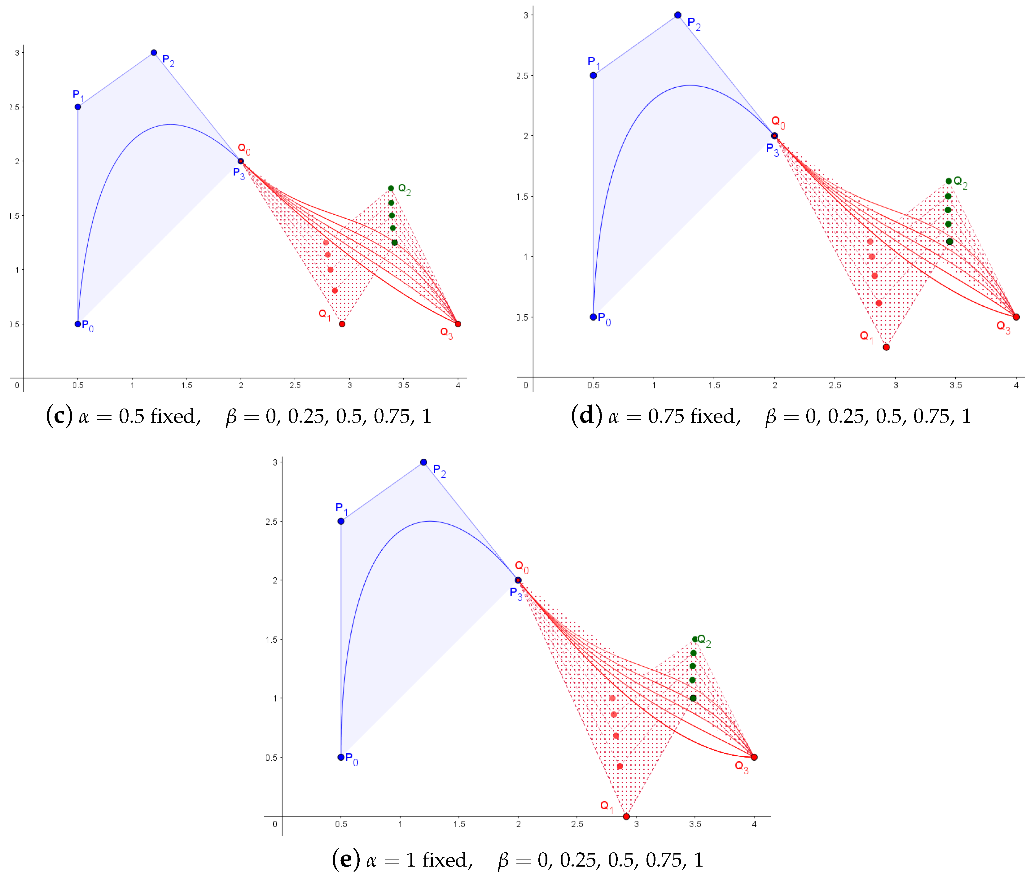
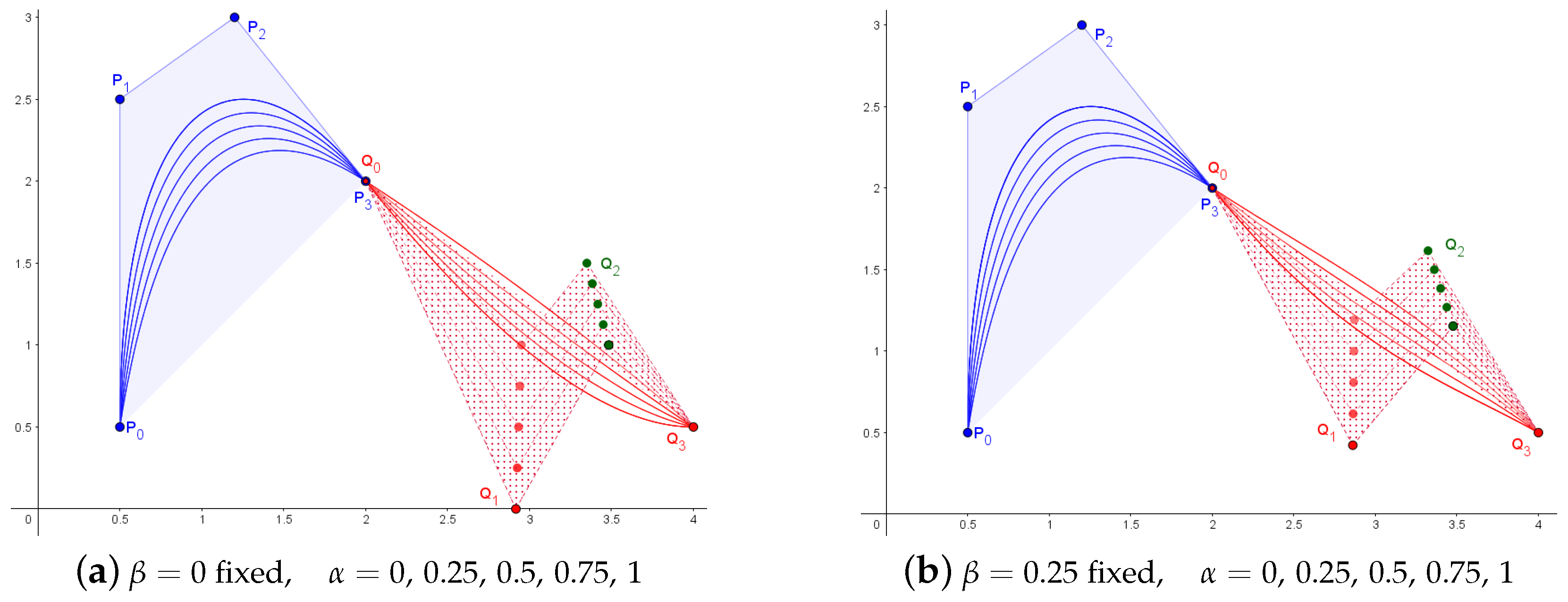
3.3. The Characteristics of $\alpha$-Bezier Curves

The following properties hold for an $n^{th}$-degree $\alpha$-Bezier curve (9):

• Terminal properties: $\mathcal{B}\left(s=0;\alpha \right)=P_0$ and $\mathcal{B}\left(s=1;\alpha \right)=P_n$, that is, the curve always starts at its first control point and ends at its last point, independent of the shape parameter $\alpha$.
  The result is followed by the end-point property of the $\alpha$-Bernstein operator.
• Convex hull: The $\alpha$-Bezier curve is a convex combination of the control points, that is, the curve $\mathcal{B}\left(s;\alpha \right)$ lies within the convex hull of the control points $\{P_0{P}_1\dots P_n\}$.
  The result is followed by the non-negativity and the partition of the unity properties of the $\alpha$-Bernstein operator.
• Geometric invariance: The $\alpha$-Bezier curve is affine-independent, that is, the curve $\mathcal{B}\left(s;\alpha \right)$ does not vary according to the change in coordinates no matter what the shape parameter is.
  The result is followed by the non-negativity and the partition of unity properties of the $\alpha$-Bernstein operator.
• Symmetry: The same $\alpha$-Bezier curve is obtained by re-indexing the control net from $\{P_0{P}_1\dots P_n\}$ to $\{P_n{P}_{n-1}\dots P_0\}$.
  The result is followed by the symmetry property of the $\alpha$-Bernstein operator.
• Geometric properties at the end-points: The tangent line of the $n^{th}$-degree $\alpha$-Bezier curve at its first control point $P_0$ lies in the plane spanned by the first three control points $sp\{P_0,P_1,P_2\}$ with the given relation as follows:

  $${\mathcal{B}}^{\prime }\left(s;\alpha \right){|}_{s=0}=(1-\alpha )\Delta P_1+(n-1+\alpha )\Delta P_0,$$

  and similarly, the tangent line at the curve’s last control point $P_n$ lies in the plane spanned by the last three control points $sp\{P_{n-2},P_{n-1},P_n\}$ with the following relation:

  $${\mathcal{B}}^{\prime }\left(s;\alpha \right){|}_{s=1}=(1-\alpha )\Delta P_{n-2}+(n-1+\alpha )\Delta P_{n-1},$$

  where $\Delta P_i=P_{i+1}-P_i$.
  Proof. 

  By taking the derivative of (9) at $s=0$ and recalling the property of the derivatives at the corner points for the $\alpha$-Bernstein operator, we obtain

  $$\begin{array}{cc}\hfill {\mathcal{B}}^{\prime }\left(s=0;\alpha \right)& =\sum _{k=0}^n{p}_k^n{\left(0;\alpha \right)}^{\prime }{P}_k\hfill \\ & =\left(1-\left(\alpha +n\right)\right)P_0+\left(n-2\left(1-\alpha \right)\right)P_1+\left(1-\alpha \right)P_2\hfill \\ & =(1-\alpha )\Delta P_1+(n-1+\alpha )\Delta P_0,\hfill \end{array}$$

  which completes the proof. Analogous to this, the proof can be induced at $s=1$. □
• Second-order derivatives at the end-points: The second derivative at the end-points of the $n^{th}$-degree $\alpha$-Bezier curve is given by the following:

  $$\begin{array}{cc}\hfill {\mathcal{B}}^{″}\left(s=0;\alpha \right)& =2\left(n-2\right)\left(1-\alpha \right){\Delta }^2{P}_1+\left(n-1\right)\left(n-2\left(1-\alpha \right)\right){\Delta }^2{P}_0\hfill \\ \hfill {\mathcal{B}}^{″}\left(s=1;\alpha \right)& =2\left(n-2\right)\left(1-\alpha \right){\Delta }^2{P}_{n-3}+\left(n-1\right)\left(n-2\left(1-\alpha \right)\right){\Delta }^2{P}_{n-2}\hfill \end{array},$$

  where ${\Delta }^2{P}_i=\Delta P_{i+1}-\Delta P_i=P_{i+2}-2P_{i+1}+P_i$.
  Proof. 

  The proof follows according to the relations given in (8). □

3.4. Subdivision of the $\alpha$-Bezier Curves

Definition 5. 

Let $\mathcal{B}\left(s_0;\alpha \right)$ be a fixed point on the α-Bezier curve with given control points $P_k\in {\mathbb{R}}^2(/{\mathbb{R}}^3)$ where $k=0,1,\dots ,n$, and $s_0,\alpha \in [0,1]$. Then, for $P_k=P_k^0$, a de Casteljau-like subdivision algorithm is given by the following scheme:

Figure 2 below demonstrates the construction of the $\alpha$-Bezier curve using de Casteljau’s algorithm. The effect of the shape parameter is visualized at three different fixed points, $s_0=0.25,=0.50,=0.75$, on the curve. The algorithm clearly indicates that if the parameter $\alpha$ is increased from $\alpha =0.0$ to $\alpha =1.0$ by $0.2$, a further iteration occurs (as shown in the green ellipses), which ultimately adjusts the shape of the $\alpha$-Bezier curve.

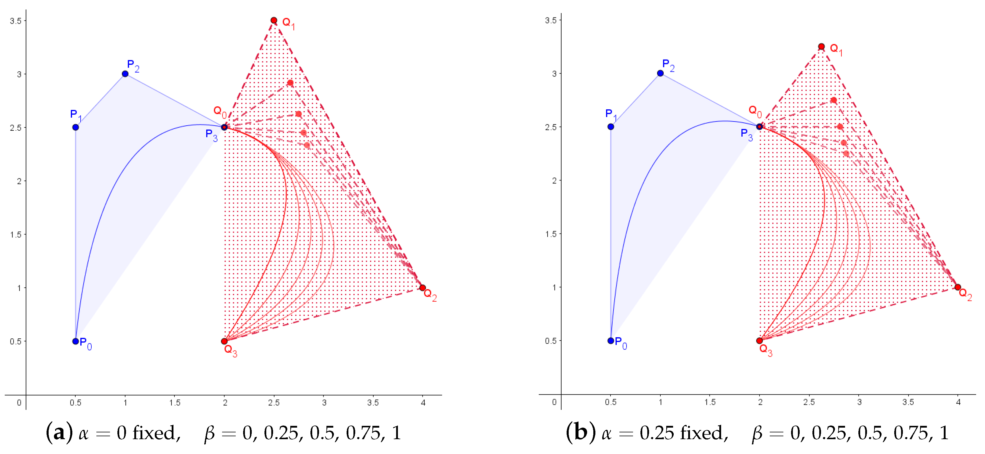
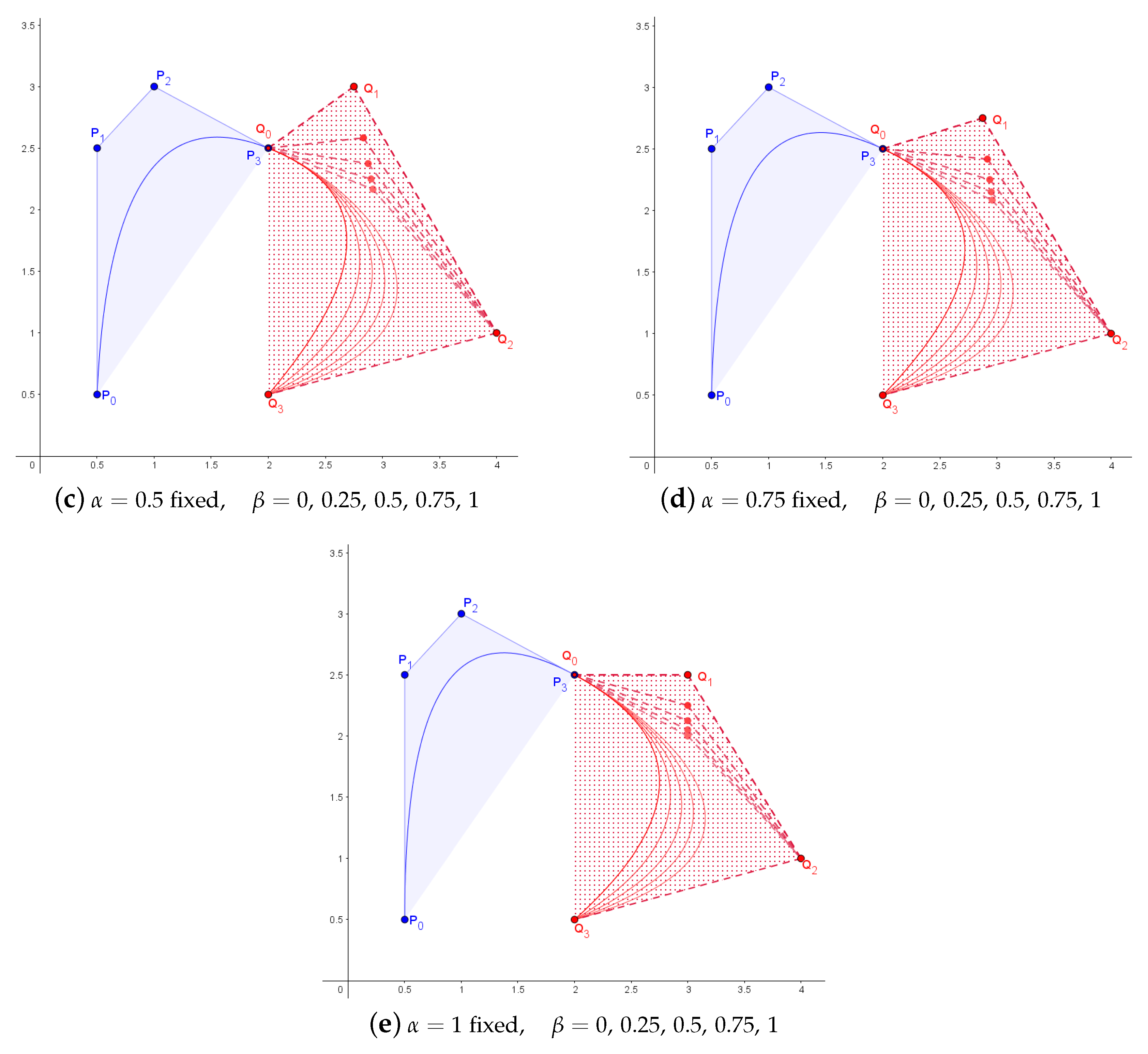
3.5. Parametric Continuity Conditions for $\alpha$-Bezier Curves

In CAGD, complex-shaped designs require many control points. In such cases, the Bezier method results in a higher degree of polynomial curves. This situation causes problems in terms of the computational costs, memory, and time. Therefore, the practical method is to join the curves by considering the required continuity conditions. In most of the cases, a smooth connection is obtained according to $C^2$ continuity, which also guarantees the $C^0$ and $C^1$ continuities. Let us consider the following two $\alpha$-Bezier curves:

$$\left\{\begin{array}{cc}\hfill {\mathcal{B}}_1\left(s;\alpha \right)& =\sum _{i=0}^n{p}_i^n\left(s;\alpha \right)P_i,2\le n\hfill \\ \hfill {\mathcal{B}}_2\left(s;\beta \right)& =\sum _{j=0}^m{q}_j^m\left(s;\beta \right)Q_j,2\le m\hfill \end{array}\right.,$$

where $p_i^n\left(s;\alpha \right)$ and $q_j^m\left(s;\beta \right)$ are the generalized $\alpha$-Bernstein operators of degree n and m with different shape parameters $\alpha ,\beta \in \left[0,1\right]$, respectively. The control points for the curve ${\mathcal{B}}_1\left(s;\alpha \right)$ are $P_i,i=0,\dots ,n$, whereas for the curve ${\mathcal{B}}_2\left(s;\beta \right)$, they are $Q_j,j=0,\dots ,m$.

Theorem 1. 

Given two α-Bezier curves ${\mathcal{B}}_1\left(s;\alpha \right)$ and ${\mathcal{B}}_2\left(s;\beta \right)$, for the parametric continuity conditions of $C^0$, $C^1$, and $C^2$, the following relations exist at the joint points of each curve:

$$\begin{array}{cc}\hfill C^0\Rightarrow & Q_0=P_n\hfill \\ \hfill C^1\Rightarrow & Q_1={\displaystyle \frac{\left(\beta -1\right)Q_2+\left(2\left(n-1\right)+\alpha +\beta \right)P_n+\left(2\left(1-\alpha \right)-n\right)P_{n-1}-\left(1-\alpha \right)P_{n-2}}{n-2\left(1-\beta \right)}}\hfill \\ \hfill C^2\Rightarrow & Q_2={\displaystyle \frac{{\zeta }_0{Q}_3+{\zeta }_1{P}_n+{\zeta }_2{P}_{n-1}+{\zeta }_3{P}_{n-2}+{\zeta }_4{P}_{n-3}}{n^2\left(2\beta -n-1\right)+6\beta \left({\alpha }_2\left(n-2\right)-3n+4\right)+12\left(n-1\right)}}\hfill \end{array}$$

where

$$\begin{array}{cc}\hfill {\zeta }_0& =-2\left(n-2\right)\left(1-\beta \right)\left(n-2+2\beta \right)=-{\zeta }_4,\hfill \\ \hfill {\zeta }_1& =2\left(\left(n-2\right)\left({\beta }^2+\alpha \beta -\alpha \right)+\left(1-n\right)\left(n^2+5\beta -4\right)+\beta \right),\hfill \\ \hfill {\zeta }_2& =-2\left(n-2\right)\left(4\left(\alpha \beta +1\right)+\left(n-4\right)\left(\alpha +\beta \right)-2n\right),\hfill \\ \hfill {\zeta }_3& =n^2\left(4\alpha +2\beta +n-1\right)+10\alpha \beta \left(n-2\right)-6n\left(3\alpha +2\beta +n\right)+20\left(\alpha +\beta +n-1\right).\hfill \end{array}$$

Proof. 

It is clear that the curves should meet at their end-points for a continuty condition of $C^0$, that is, ${\mathcal{B}}_1\left(1;\alpha \right)={\mathcal{B}}_2\left(0;\beta \right)$. Thus, the proof is clear from the terminal property of the $\alpha$-Bezier curves.

Further, for the $C^1$ continuity condition, the tangent lines should meet at the curve’s end-points while the condition of $C^0$ holds still. That is, ${\mathcal{B}}_1^{\prime }\left(1;\alpha \right)={\mathcal{B}}_2^{\prime }\left(0;\beta \right)$. By using the geometric properties at the end-points, we have

$$\left(1-\alpha \right)\Delta P_{n-2}+\left(n-\left(1-\alpha \right)\right)\Delta P_{n-1}=\left(1-\beta \right)\Delta Q_1+\left(n-\left(1-\beta \right)\right)\Delta Q_0.$$

Hence, with simple algebraic manipulations, we complete the proof.

Parallel to the above, the parametric continuity condition of $C^2$ can be obtained according to the relation ${\mathcal{B}}_1^{″}\left(1;\alpha \right)={\mathcal{B}}_2^{″}\left(0;\beta \right)$. Upon using the geometric properties at the end-points for the $\alpha$-Bezier curves, we obtain the following equation:

$$\begin{array}{c}{\displaystyle 2\left(n-2\right)\left[\left(1-\alpha \right){\Delta }^2{P}_{n-3}-\left(1-\beta \right){\Delta }^2{Q}_1\right]=}\hfill \\ {\displaystyle \left(1-n\right)\left[\left(n-2\left(1-\alpha \right)\right){\Delta }^2{P}_{n-2}-\left(n-2\left(1-\beta \right)\right){\Delta }^2{Q}_0\right].}\hfill \end{array}$$

By considering the $C^0$ and $C^1$ continuity conditions, along with the last relation, the proof is completed. □

In Figure 3 and Figure 4, two adjacent $\alpha$-Bezier curves possessing $C^1$ continuity are illustrated. Particularly, in Figure 3, adjusting the shape parameter of the second curve results in a local change when the first curve’s parameter is fixed. However, in Figure 4, the variation in the first curve’s parameter produces a global change in the curves even if the second curve’s parameter remains constant.

Analogous to the previous one, a similar argument for local and global changes exists for adjacent $\alpha$-Bezier curves with $C^2$ continuity (see Figure 5 and Figure 6).

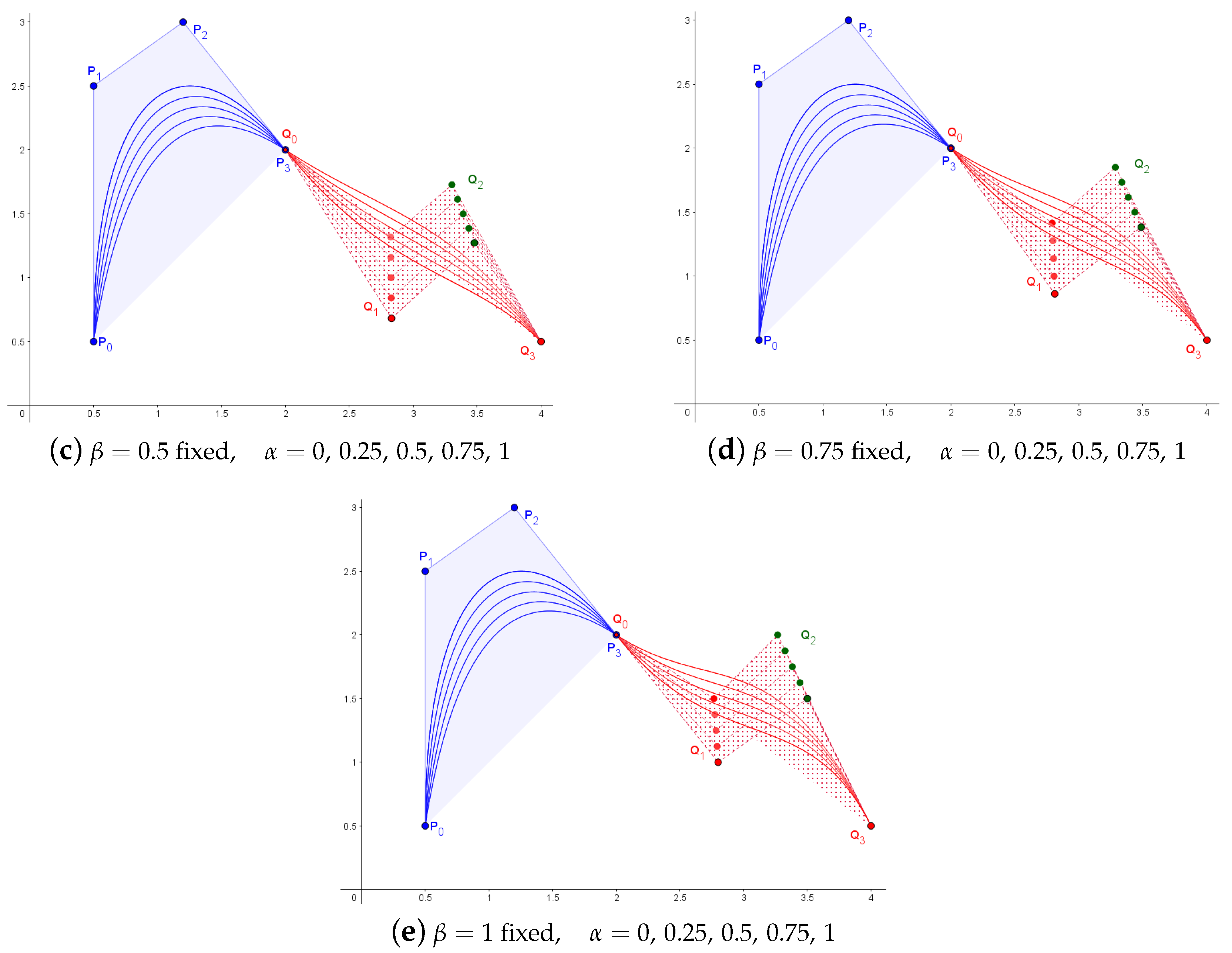
3.6. Cross-Sectional Design Surfaces with $\alpha$-Bezier Curves

In this section, a set of engineering surfaces has been defined. Such engineering surfaces are also called cross-sectional designs, as they are crossed by two curves, namely a profile curve and a trajectory curve. Thus, we first construct a tensor product surface and then ruled, rotational, swept, and swung surfaces by using new novel $\alpha$-Bezier curves with varying parameters.

3.7. Tensor Product $\alpha$-Bezier Surfaces

Definition 6. 

For $u,v\in [0,1],$ and given control points $P_{ij}\in {\mathbb{R}}^3$ where $i=0,\dots ,n$ and $j=1,\dots ,m$, the two shape parameters of an $(n,m)$-degree tensor product α-Bezier surface are defined as follows:

$${\mathcal{S}}_{i,j}^{n,m}(u;{\alpha }_1,v;{\alpha }_2)=\sum _{i=0}^n\sum _{j=0}^m{P}_{ij}{p}_i^n\left(u;{\alpha }_1\right)p_j^m\left(v;{\alpha }_2\right),$$

where ${\alpha }_1,{\alpha }_2\in [0,1]$, and $p_i^n\left(u;{\alpha }_1\right)$ and $p_j^m\left(v;{\alpha }_2\right)$ are the generalized α-Bernstein operators, respectively.

3.8. Properties of $\alpha$-Bezier Surfaces

$\alpha$-Bezier surfaces depict the similar properties to those of $\alpha$-Bezier curves. Therefore, without the need for a proof, we list these properties as follows:

• Convex hull property: The $\alpha$-Bezier surface $\mathcal{S}\left(u,v;{\alpha }_1,{\alpha }_2\right)$ lies in the convex hull defined by its control net;
• Affine invariance Applying an affine transformation to an $\alpha$-Bezier surface is the same as the surface being constructed with the transformed control points;
• Isoparametric curves: Since the $\alpha$-Bezier surface is built using a tensor product, any isoparametric curves at a point on the surface result in a new $\alpha$-Bezier curve;
• Boundary curves: As special kinds of isoparametric curves, the four boundary curves of the $\alpha$-Bezier surface, by setting $u=0$, $u=1$, $v=0$, and $v=1$, correspond to $\alpha$-Bezier curves.

The tensor product $\alpha$-Bezier surfaces with different values for the shape parameters ${\alpha }_1$ and ${\alpha }_2$ are illustrated in Figure 7.

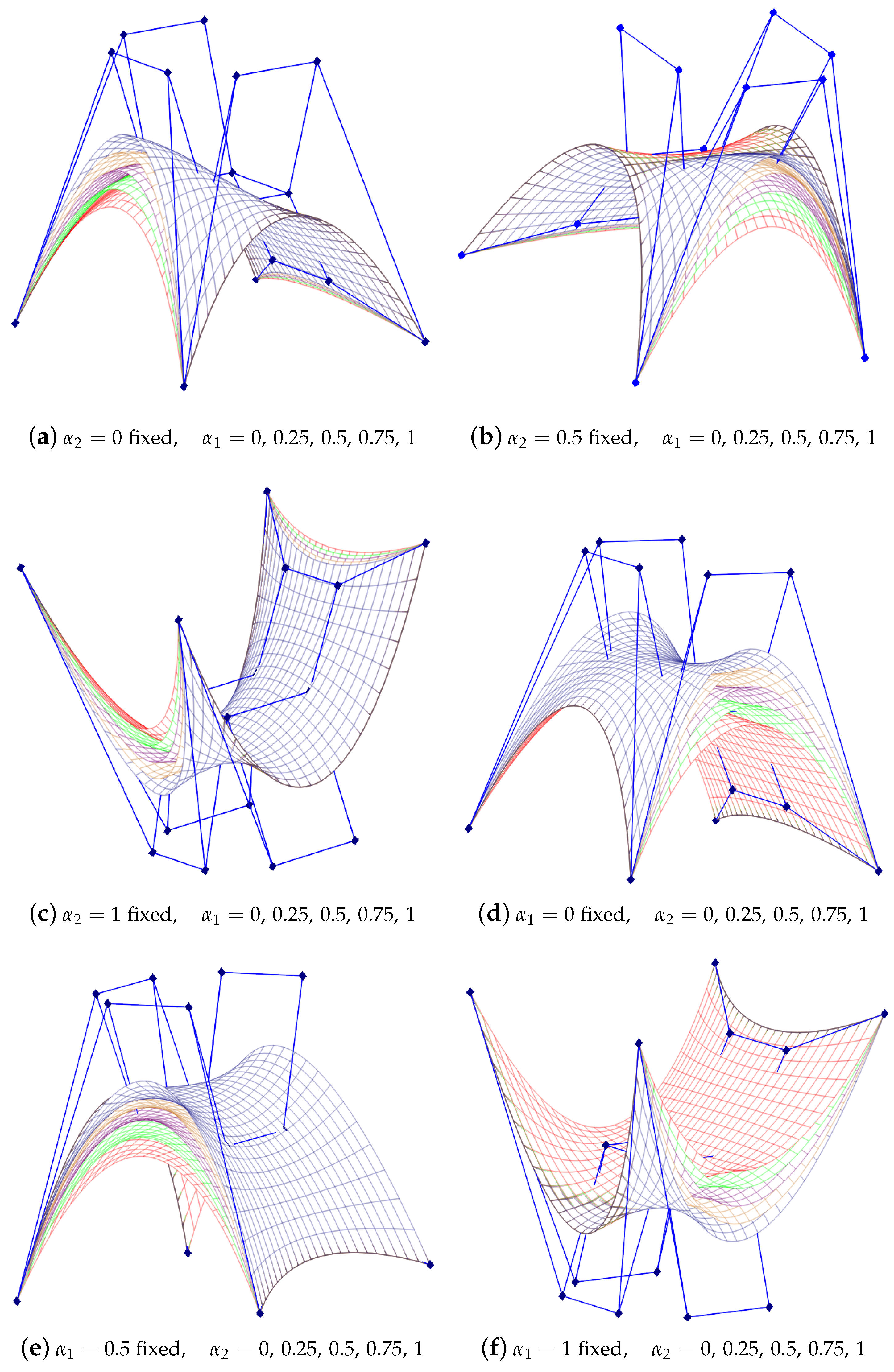
3.9. Ruled Surfaces Using $\alpha$-Bezier Curves

A ruled surface is a kind of surface which has perhaps the simplest structure compared to that of other surface types. Contrary to its conventional parametrization, a ruled surface can be formed with infinitely many lines between two curves Thus, as a cross-sectional design, a ruled surface can be defined as follows:

Definition 7. 

For $u,v\in [0,1],$ and given control points $P_i\in {\mathbb{R}}^3,$ $i=0,\dots ,n$, and $Q_j\in {\mathbb{R}}^3,j=0,\dots ,m$, let the two α-Bezier curves of degree n and m be defined as ${\mathcal{B}}_1(u;{\alpha }_1)={\sum }_{i=0}^n{p}_i^n\left(u;{\alpha }_1\right)P_i$ and ${\mathcal{B}}_2(u;{\alpha }_2)={\sum }_{j=0}^n{p}_j^m\left(u;{\alpha }_2\right)Q_j$, respectively. Then, the surface formed by the family of lines passing from the curve ${\mathcal{B}}_1$ to the curve ${\mathcal{B}}_2$ at their corresponding points is called a ruled surface. Thus, the parametric equation of a ruled surface can be expressed through linear interpolation as proposed in [33] as follows:

$$\chi (u,v;{\alpha }_1,{\alpha }_2)=(1-v){\mathcal{B}}_1(u;{\alpha }_1)+v{\mathcal{B}}_2(u;{\alpha }_2).$$

(10)

Remark 1. 

Note that if one of the curves ${\mathcal{B}}_2(u;{\alpha }_2)$ is a translation of the other curve by a given vector $\overrightarrow{\omega }$ such that ${\mathcal{B}}_2(u;{\alpha }_2)={\mathcal{B}}_1(u;{\alpha }_1)+\overrightarrow{\omega }$, then the generated ruled surface simply forms a cylinder with given appropriate control points. Further, if one of the curves, say ${\mathcal{B}}_2(u;{\alpha }_2)$, is degenerated to a point, then a special ruled surface cone is constructed. To indicate the parameter effect, half of these special ruled surfaces are illustrated in Figure 8, as well as a regular ruled surface with two closed planar α-Bezier curves each lying on the $xy$- and $xz$- planes.

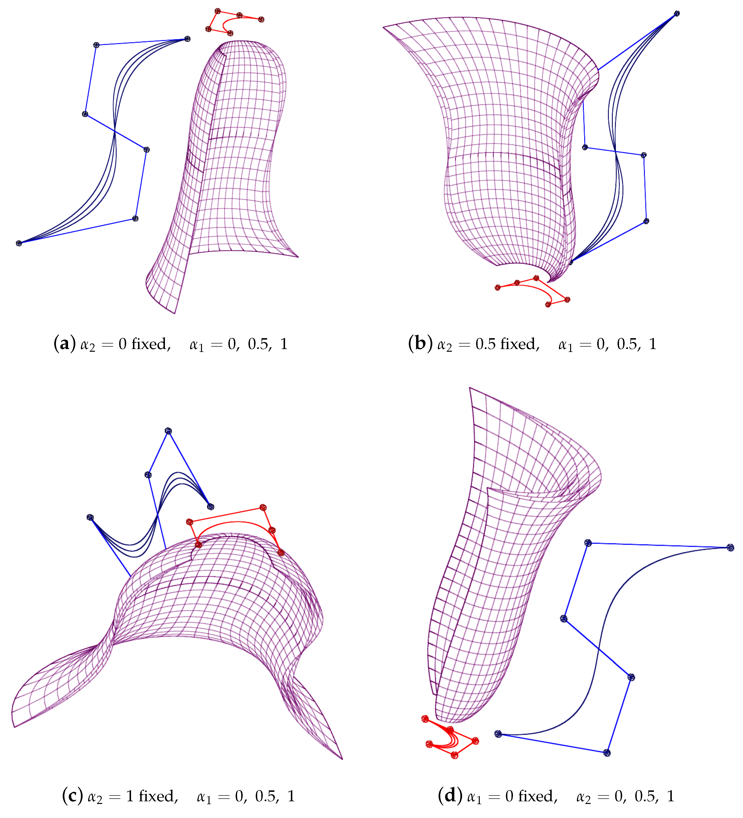
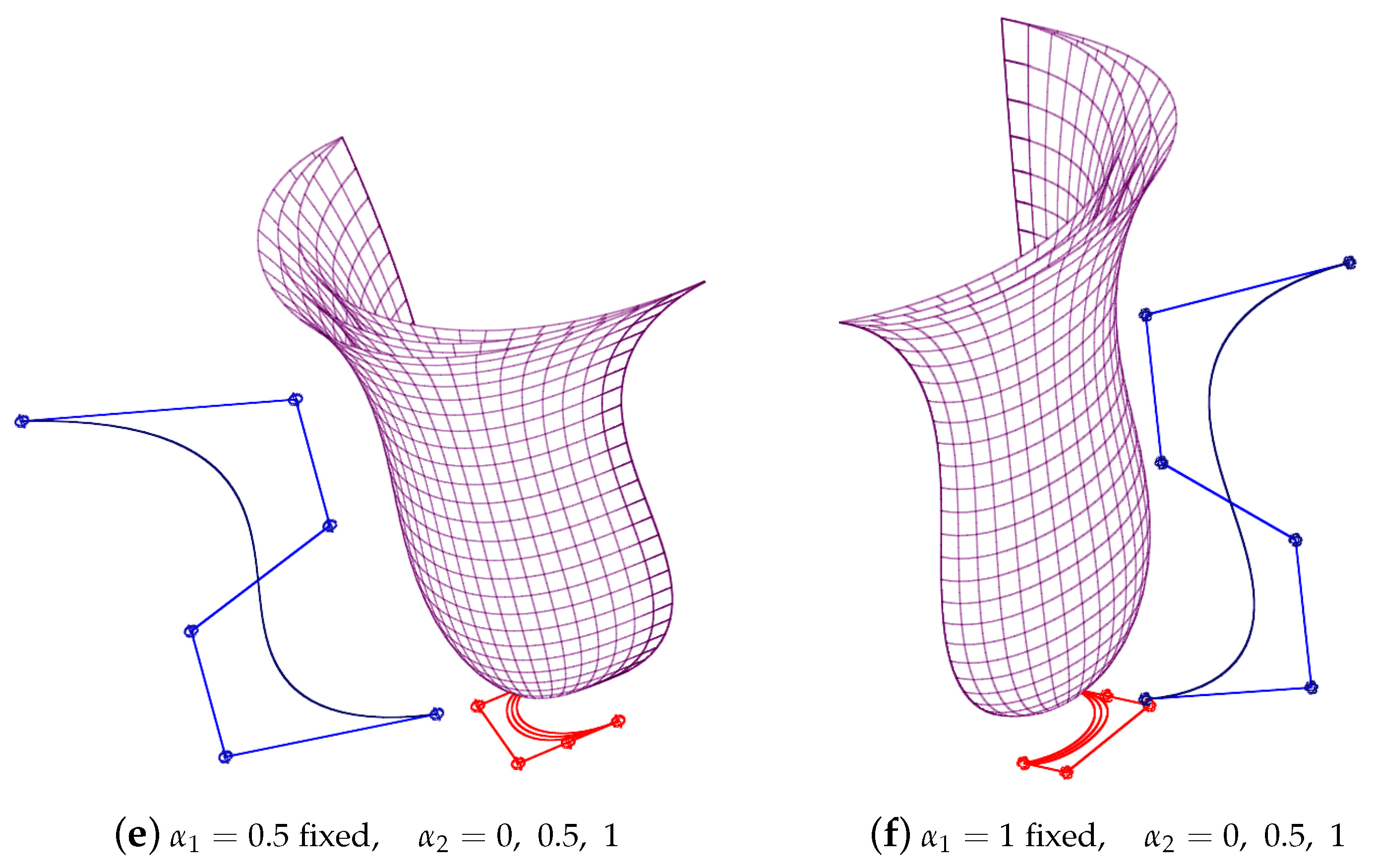
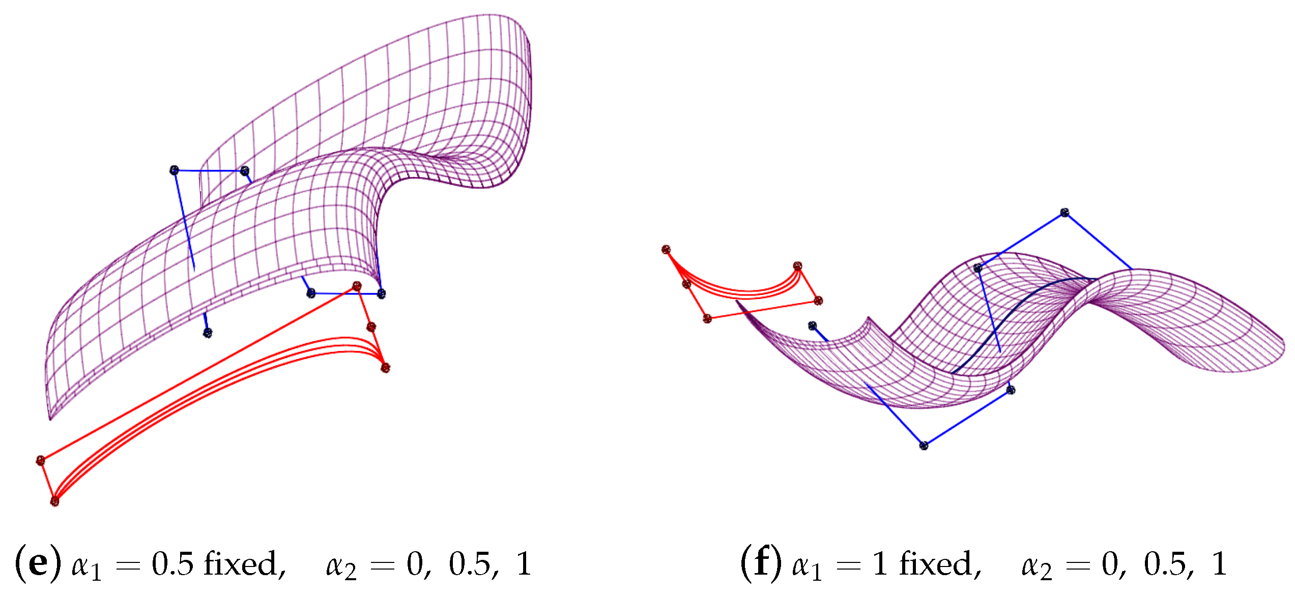
3.10. $\alpha$-Bezier Swung Surfaces

Definition 8. 

For $u,v,\in [0,1]$, and given control points $P_i\in {\mathbb{R}}^3,$ $i=0,\dots ,n$, and $Q_j\in {\mathbb{R}}^3,j=0,\dots ,m$, let the two α-Bezier curves of degree n and m denoted by $\mathcal{P}(u;{\alpha }_1)={\sum }_{i=0}^n{p}_i^n\left(u;{\alpha }_1\right)P_i$ and $\mathcal{T}(v;{\alpha }_2)={\sum }_{j=0}^n{p}_j^m\left(v;{\alpha }_2\right)Q_j$ be the profile and trajectory curves, respectively. If the profile curve is formed in the $xz$-plane, that is, $\mathcal{P}(u;{\alpha }_2)=(P_x(u;{\alpha }_1),0,P_z(u;{\alpha }_1))$, and if the trajectory curve is from the $xy$-plane, that is, $\mathcal{T}=(T_x(v;{\alpha }_2),T_y(v;{\alpha }_2),0)$, then the swung surface with a scaling factor $k\in \mathbb{R}$ is defined as follows:

$$\mathbb{S}(u,v;{\alpha }_1,{\alpha }_2)=\left(k{P}_x(u;{\alpha }_1)T_x(v;{\alpha }_2),k{P}_x(u;{\alpha }_1)T_y(v;{\alpha }_2),P_z(u;{\alpha }_1)\right).$$

The variation effect of the shape parameters on a swung $\alpha$-Bezier surface is illustrated in Figure 9.

3.11. $\alpha$-Bezier Swept Surfaces

Definition 9. 

Let us consider the two curves $\mathcal{P}(u;{\alpha }_1)$ and $\mathcal{T}(v;{\alpha }_2)$, as defined before in Definition 8. Then, a swept (sweeping) surface is defined by the following parametrization:

$$S(u,v;{\alpha }_1,{\alpha }_2)=\mathcal{T}(v;{\alpha }_2)+M\left(v\right)\mathcal{P}(u;{\alpha }_1),$$

where $M\left(v\right)$ is a transformation matrix at v [34].

Figure 10 illustrates the change in the surface layer by tuning the shape parameters.

In order to test the efficiency of $\alpha$-Bezier curves for designing models, a 3d model is created to be printed with a 3d printer. The following, Figure 11, shows a decorative model of a swept surface and its 3d printing stage.

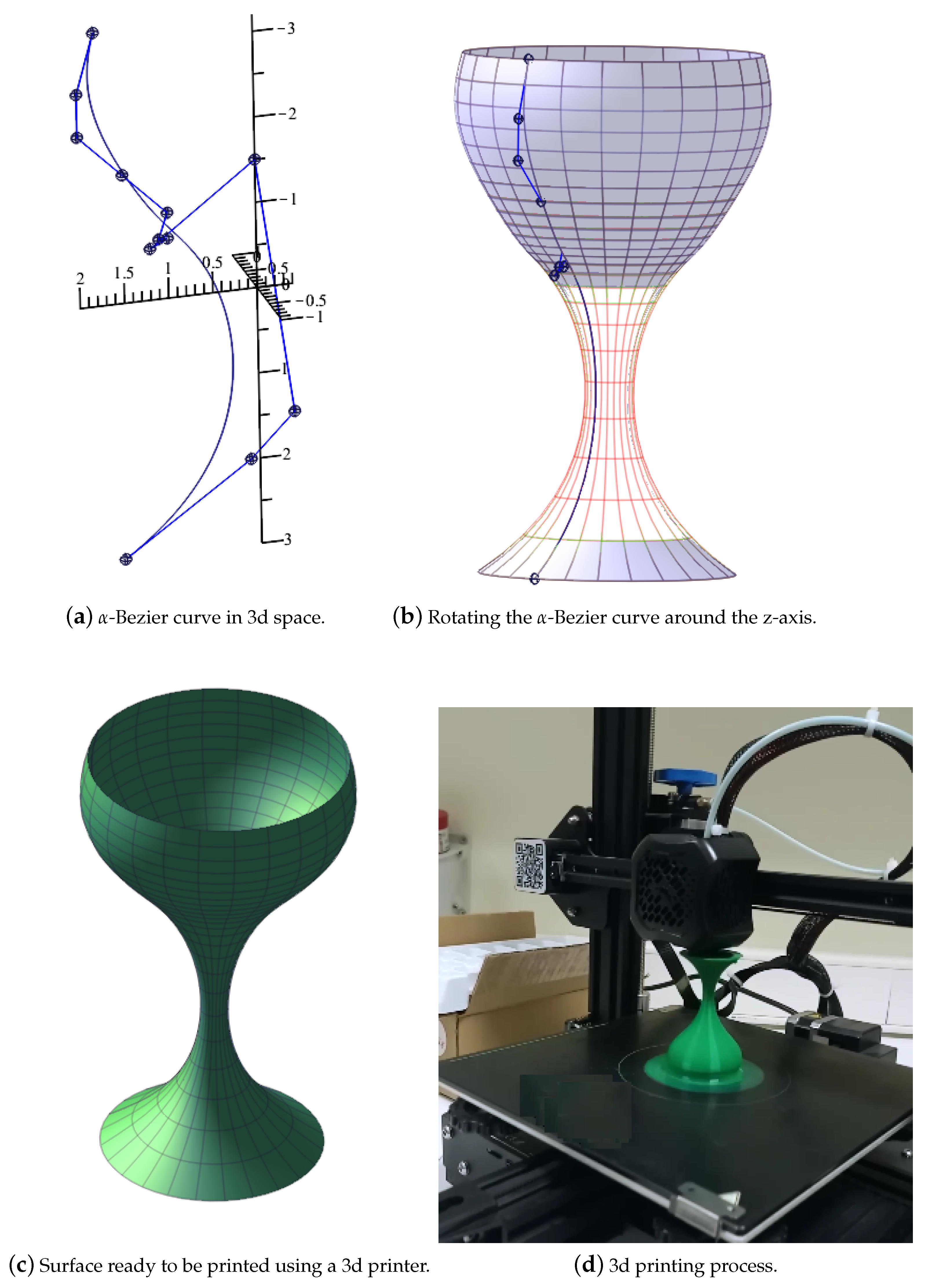
3.12. Rotational Surfaces Using $\alpha$-Bezier Curves

Rotational surfaces are a very popular surface type since they are easy to design and are frequently used in CAGD. To create a surface of rotation, one needs a planar profile curve and an axis on which the rotation to be applied to the curve can occur. Generally, surfaces are created in three-dimensional Euclidean space by taking the rotation axis as the z-axis [33,34].

Definition 10. 

For $u\in [0,1]$, and given control points $P_i(x_i,0,z_i)\in {\mathbb{R}}^3,$ where $i=0,\dots ,n$, let a planar α-Bezier curve of degree n on the $xz$ plane defined by $\mathcal{B}(u;\alpha )={\sum }_{i=0}^n{p}_i^n\left(u;\alpha \right)P_i$ be the profile curve. If the rotation axis is considered the z-axis, then a rotational-surface-based $\mathcal{B}(u;\alpha )$ is defined as follows:

$${\mathcal{S}}_r(u,\theta )={\mathcal{R}}_z\left(\theta \right)·\mathcal{B}(u;\alpha ),$$

(11)

where

$${\mathcal{R}}_z\left(\theta \right)=\left(\begin{array}{ccc}cos\left(\theta \right)& -sin\left(\theta \right)& 0\\ sin\left(\theta \right)& cos\left(\theta \right)& 0\\ 0& 0& 1\end{array}\right)$$

(12)

is the rotation matrix according to the z-axis.

However, sometimes, the rotation matrix given by Equation (12) causes complexity in the calculation and cutting errors due to the trigonometric expressions it contains; thus, the rotational motion is also achieved using the two following symmetric half-surfaces whose parametrizations were previously outlined in [33] as follows:

$$\begin{array}{cc}\hfill {}^1\mathcal{S}_r(u,v;\alpha )=& \left\{{\displaystyle \frac{1-2v}{v^2+{(v-1)}^2}}x\left(\mathcal{B}(u;\alpha )\right),{\displaystyle \frac{2v(1-v)}{v^2+{(v-1)}^2}}x\left(\mathcal{B}(u;\alpha )\right),z\left(\mathcal{B}(u;\alpha )\right)\right\}\hfill \\ \hfill {}^2\mathcal{S}_r(u,v;\alpha )=& \left\{{\displaystyle \frac{1-2v}{v^2+{(v-1)}^2}}x\left(\mathcal{B}(u;\alpha )\right),-{\displaystyle \frac{2v(1-v)}{v^2+{(v-1)}^2}}x\left(\mathcal{B}(u;\alpha )\right),z\left(\mathcal{B}(u;\alpha )\right)\right\}\hfill \end{array}.$$

(13)

Figure 12 illustrates half of the rotational surface by using ${}^1\mathcal{S}_r(u,v;\alpha )$ in order to show the effect of the change in parameter $\alpha$.

Moreover, using an $\alpha$-Bezier curve, the design of a chalice is presented in Figure 13. This model was also printed using a 3d printer so that the efficiency of creation could be validated.

4. Conclusions

In the current research as a whole, we have presented an examination of the one shape parameter of a generalized $\alpha$-Bernstein operator concerning its efficacy in generating Bezier-like curves and surfaces. A novel depiction of an $\alpha$-Bernstein operator, along with other practical representations, has been given, which can prove valuable in the implementation of the de Casteljau-like subdivision algorithm. We have also covered a discussion of the conditions of parametric continuity to join two $\alpha$-Bezier curves in order to enhance the generation of intricately shaped designs. Further, a set of cross-sectional design surfaces was constructed, along with the new $\alpha$-Bezier curves, and the parameter effects examined by providing various figures. Finally, even when the parameter range is restricted, the novel $\alpha$-Bezier curves and surfaces demonstrate more edges than those of the conventional Bezier curve and surfaces. Defining a new basis with multiple shape parameters to improve the accuracy of controlling the shape of the curves and surfaces, as well as scanning almost the whole area of a control polygon, is of interest as future work.

References

- Böhm, W.; Farin, G.; Kahmann, J. A survey of curve and surface methods in CAGD. Comput. Aided Geom. Des. 1984, 1, 1–60. [Google Scholar] [CrossRef]
- Farin, G. Curves and Surfaces for Computer-Aided Geometric Design: A Practical Guide; Elsevier: Amsterdam, The Netherlands, 2014. [Google Scholar]
- Li, C.; Zhu, C. Designing developable C-Bézier surface with shape parameters. Mathematics 2020, 8, 402. [Google Scholar] [CrossRef]
- Oruç, H.; Phillips, G.M. q-Bernstein polynomials and Bézier curves. J. Comput. Appl. Math. 2003, 151, 1–12. [Google Scholar] [CrossRef]
- Wang, W.; Wang, G. Bézier curves with shape parameter. J. Zhejiang Univ.-Sci. 2005, 6, 497–501. [Google Scholar]
- Ye, Z.; Long, X.; Zeng, X.M. Adjustment algorithms for Bézier curve and surface. In Proceedings of the 2010 5th International Conference on Computer Science & Education, Hefei, China, 24–27 August 2010; pp. 1712–1716. [Google Scholar]
- Yan, L.L.; Liang, J.F. An extension of the Bézier model. Appl. Math. Comput. 2011, 218, 2863–2879. [Google Scholar] [CrossRef]
- Qin, X.; Hu, G.; Zhang, N.; Shen, X.; Yang, Y. A novel extension to the polynomial basis functions describing Bézier curves and surfaces of degree n with multiple shape parameters. Appl. Math. Comput. 2013, 223, 1–16. [Google Scholar] [CrossRef]
- Cai, Q.B.; Zhou, G. Properties of (λ, q)-Bezier Curves and Surfaces. In Proceedings of the 2018 IEEE 4th International Conference on Computer and Communications (ICCC), Chengdu, China, 7–10 December 2018; pp. 2228–2232. [Google Scholar]
- Han, X.A.; Ma, Y.; Huang, X. A novel generalization of Bézier curve and surface. J. Comput. Appl. Math. 2008, 217, 180–193. [Google Scholar] [CrossRef]
- Zhang, J. C-curves: An extension of cubic curves. Comput. Aided Geom. Des. 1996, 13, 199–217. [Google Scholar] [CrossRef]
- Pottmann, H. The geometry of Tchebycheffian spines. Comput. Aided Geom. Des. 1993, 10, 181–210. [Google Scholar] [CrossRef]
- Chen, Q.; Wang, G. A class of Bézier-like curves. Comput. Aided Geom. Des. 2003, 20, 29–39. [Google Scholar] [CrossRef]
- Lü, Y.; Wang, G.; Yang, X. Uniform hyperbolic polynomial B-spline curves. Comput. Aided Geom. Des. 2002, 19, 379–393. [Google Scholar] [CrossRef]
- Zhu, Y.; Han, X. Curves and surfaces construction based on new basis with exponential functions. Acta Appl. Math. 2014, 129, 183–203. [Google Scholar] [CrossRef]
- Zhu, Y.; Liu, Z. A class of trigonometric Bernstein-type basis functions with four shape parameters. Math. Probl. Eng. 2019, 2019, 9026187. [Google Scholar] [CrossRef]
- Majeed, A.; Abbas, M.; Sittar, A.A.; Kamran, M.; Tahseen, S.; Emadifar, H. New Cubic Trigonometric Bezier-Like Functions with Shape Parameter: Curvature and Its Spiral Segment. J. Math. 2021, 2021, 6330649. [Google Scholar] [CrossRef]
- Yılmaz Ceylan, A. Construction of a new class of Bézier like curves. Math. Methods Appl. Sci. 2021, 44, 7659–7665. [Google Scholar] [CrossRef]
- Canlı, D.; Şenyurt, S. Bezier Like Curves by a New Basis with a Two Shape Parameters of Exponential Function. In Proceedings of the 10th International “Baskent” Congress On Physical, Engineering, and Applied Sciences, Ankara, Turkey, 28–30 October 2023; Proceedings Book. BZT Academy Pub. House: Istanbul, Türkiye, 2023; pp. 171–177. [Google Scholar]
- Canlı, D.; Şenyurt, S. A Logarithmic Basis with One-Shape Parameter To Construct Free Form Curves By Bezier Method. In Proceedings of the 5th International Acharaka Congress on Life Engineering and Applied Sciences, Izmir, Turkey, 11–13 November 2023; Proceedings Book. BZT Academy Pub. House: Istanbul, Türkiye, 2023; pp. 177–185. [Google Scholar]
- Canlı, D.; Şenyurt, S. Cubic Bezier-Like Curves with Two Shape Parameters Of Trigonometric Tangent Function. In Proceedings of the International Euroasia Congress on Scientific Researches and Recent Trends XII, Ankara, Türkiye, 29–30 November 2023; pp. 893–903. [Google Scholar]
- Fang, M.; Wang, G. w-Bézier. In Proceedings of the 10th IEEE International Conference on Computer-Aided Design and Computer Graphics, Chengdu, China, 18–21 August 2007; pp. 38–42. [Google Scholar]
- Constantini, P.; Lyche, T.; Manni, C. On a class of weak Tchebycheff systems. Numer. Math. 2005, 101, 333–354. [Google Scholar] [CrossRef]
- Schumaker, L. Spline Functions: Basic Theory; Cambridge University Press: Cambridge, UK, 2007. [Google Scholar]
- Chu, L.; Zeng, X.M. Constructing curves and triangular patches by Beta functions. J. Comput. Appl. Math. 2014, 260, 191–200. [Google Scholar] [CrossRef]
- Goldman, R.N. Pólya’s urn model and computer aided geometric design. SIAM J. Algebr. Discret. Methods 1985, 6, 1–28. [Google Scholar] [CrossRef]
- Cheng, F.; Kazadi, A.N.; Lin, A.J. Beta-Bezier Curves. Comput. Aided Des. Appl. 2021, 18, 1265–1278. [Google Scholar] [CrossRef]
- Levent, A.; Şahin, B. Beta Bezier Curves. Appl. Comput. Math. 2019, 18, 79–94. [Google Scholar]
- Cai, Q.B.; Lian, B.Y.; Zhou, G. Approximation properties of λ-Bernstein operators. J. Inequalities Appl. 2018, 2018, 61. [Google Scholar] [CrossRef] [PubMed]
- Kadak, U.; Özger, F. A numerical comparative study of generalized Bernstein-Kantorovich operators. Math. Found. Comput. 2021, 4, 311. [Google Scholar] [CrossRef]
- Chen, X.; Tan, J.; Liu, Z.; Xie, J. Approximation of functions by a new family of generalized Bernstein operators. J. Math. Anal. Appl. 2017, 450, 244–261. [Google Scholar] [CrossRef]
- Farouki, R.T. The Bernstein polynomial basis: A centennial retrospective. Comput. Aided Geom. Des. 2012, 29, 379–419. [Google Scholar] [CrossRef]
- Hu, G.; Wu, J.; Qin, X. A novel extension of the Bézier model and its applications to surface modeling. Adv. Eng. Softw. 2018, 125, 27–54. [Google Scholar] [CrossRef]
- Zhao, Y.; Zhou, Y.; Lowther, J.L.; Shene, C.K. Cross-sectional design: A tool for computer graphics and computer-aided design courses. In FIE’99 Frontiers in Education. 29th Annual Frontiers in Education Conference. Designing the Future of Science and Engineering Education. Conference Proceedings (IEEE Cat. No. 99CH37011), San Juan, PR, USA, 10–13 November 1999; IEEE: Piscataway, NJ, USA, 1999; Volume 2, p. 12B3-1. [Google Scholar]
- Canlı, D. The Geometry of Bezier Curves and Surfaces in Three-Dimensional Euclidean Space. Ph.D. Dissertation, Ordu University, Ordu, Türkiye, 2024. [Google Scholar]