Multi-Label Learning with Distribution Matching Ensemble: An Adaptive and Just-In-Time Weighted Ensemble Learning Algorithm for Classifying a Nonstationary Online Multi-Label Data Stream

Abstract

Learning from a nonstationary data stream is challenging, as a data stream is generally considered to be endless, and the learning model is required to be constantly amended for adapting the shifting data distributions. When it meets multi-label data, the challenge would be further intensified. In this study, an adaptive online weighted multi-label ensemble learning algorithm called MLDME (multi-label learning with distribution matching ensemble) is proposed. It simultaneously calculates both the feature matching level and label matching level between any one reserved data block and the new received data block, further providing an adaptive decision weight assignment for ensemble classifiers based on their distribution similarities. Specifically, MLDME abandons the most commonly used but not totally correct underlying hypothesis that in a data stream, each data block always has the most approximate distribution with that emerging after it; thus, MLDME could provide a just-in-time decision for the new received data block. In addition, to avoid an infinite extension of ensemble classifiers, we use a fixed-size buffer to store them and design three different dynamic classifier updating rules. Experimental results for nine synthetic and three real-world multi-label nonstationary data streams indicate that the proposed MLDME algorithm is superior to some popular and state-of-the-art online learning paradigms and algorithms, including two specifically designed ones for classifying a nonstationary multi-label data stream.

1. Introduction

In traditional machine learning, learning models are generally considered trained on a previously prepared dataset, and then provide prediction for future unseen instances. However, in some real-world applications, such a paradigm is not applicable any more. Actually, in these specifical applications, data can be received in the form of successive stream in which the data distribution may be altered with time. In such a scenario, the traditional static learning models would be invalid, as they always require both training and testing data satisfying an independent identically distributed hypothesis. In other words, for a nonstationary data stream, the learning models are required to update themselves constantly to adapt to the new data distribution. We call this learning paradigm online learning [1,2] and the phenomenon of the shifting data distribution concept drift [3,4,5]. 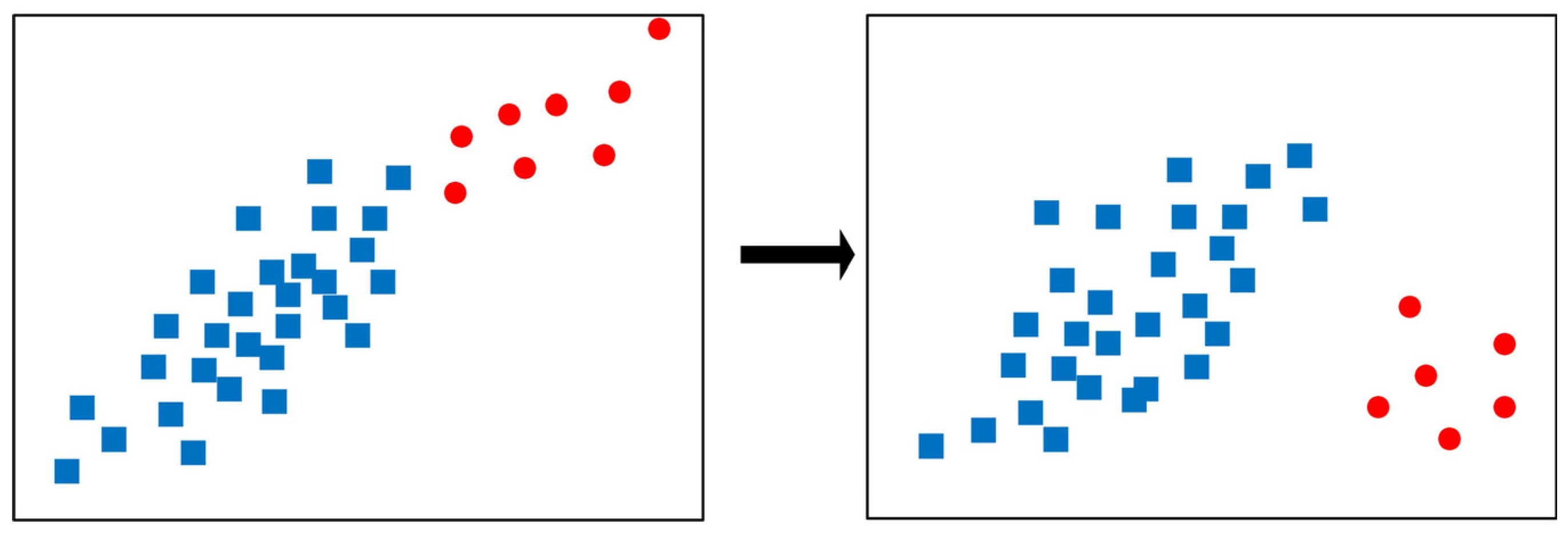Specifically, online learning has been frequently used in many real-world applications, including activity recognition [6], face recognition [7], recommendation systems [8], intrusion detection [9], fault diagnosis [10], and marketing analysis [11]. As an example of concept drift, an intrusion detection system requires persistent upgrading of itself to cope with the potentially emerging new strategies of invasion developed by hackers. In this example, once the ways of intrusion vary, that means that the feature distribution or feature–class associations are simultaneously altered, causing the originally developed intrusion detection model be out of work (see Figure 1).

As we know, learning from a data stream is significantly more difficult than learning from static data, as it needs to satisfy two basic requirements. The first one is one pass, i.e., when new data are received, we need to immediately decide to use them or abandon them, but cannot reserve and revisit them. The one pass requirement is proposed based on the hypothesis of that a real-world data stream is generally endless, and reserving all data will cause memory overflow. One pass means that once useful data have been removed, they cannot be revisited to update the current model. However, there is always a lag for estimating the usefulness of data, and thus the one pass requirement remains a critical challenge for an online learning model. The second one is that the model should adapt concept drift emerging in a data stream, which requires detecting whether a concept drift exists in time, and if it is yes, then the learning model is modified to make it coincide with the new data distribution. For the first requirement, it generally can be satisfied by one of two following solutions: the first one is to modify the conventional static learning algorithm to make it can rapidly tune the model parameters to adapt newly arrived data without considering whether they are useful [12,13], and the second one is to use ensemble learning to constantly train new learning models on newly received data and to adopt weighted voting to alleviate the effect of those models trained on useless data [14,15,16]. As for the second requirement, it can be satisfied by either simultaneously adding concept drift detectors and a forgetting mechanism in single learning model adaption [17], or adopting concept drift detectors to decide which base learners in the ensemble are useful and should be reserved, and how much weights should be assigned for them to vote, furthermore making the ensemble learning model track and adapt concept drift [18,19,20]. Obviously, it would be more flexible and robust to adopt ensemble learning than a single learner in such a scenario.

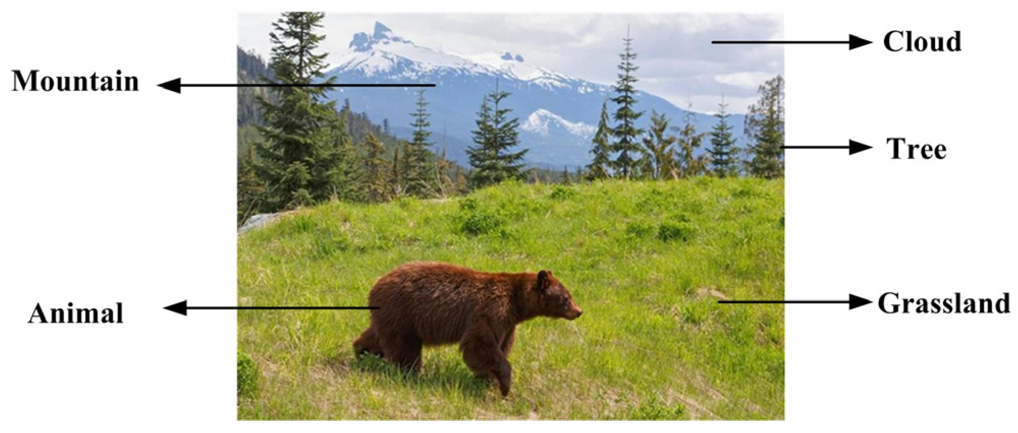
There have been lots of algorithms that can be deployed in a streaming environment. However, most of them only focus on a single-label classification problem. In context of a multi-label problem, it may require considering more factors for online learning since concept drift would become more complex [21]. In multi-label learning, the model is required to simultaneously predict multiple class labels for an instance. For example, an image may contain several class labels, such as cloud, tree, mountain, grassland, and animal (see Figure 2). While the concept drift that happens in multi-label learning tasks may be associated with the alteration of the label distribution or label associations, e.g., during the World Cup, most news simultaneously covers several topics (class labels) about sports, the economy, and tourism, but with the outbreak of a war, the news would be attracted to focus on the combination of several other topics of war, politics, humanitarianism, economy, and munitions. In such a scenario, no matter the label correlation (which class labels tend to simultaneously emerge) shift or label distribution (which class labels tend to more emerge) shift, it can be regarded as the emergence of concept drift. Therefore, when online learning meets multi-label data, the challenge would be significantly intensified.

Motivated by the issue mentioned above, we designed and developed an adaptive and just-in-time online multi-label learning algorithm named MLDME (multi-label learning with distribution matching ensemble). Specifically, it partially inherits our previously proposed DME (distribution matching ensemble) algorithm [22]. DME first uses a Gaussian mixture model (GMM) [23] to accurately measure the data distribution of each received data chunk. 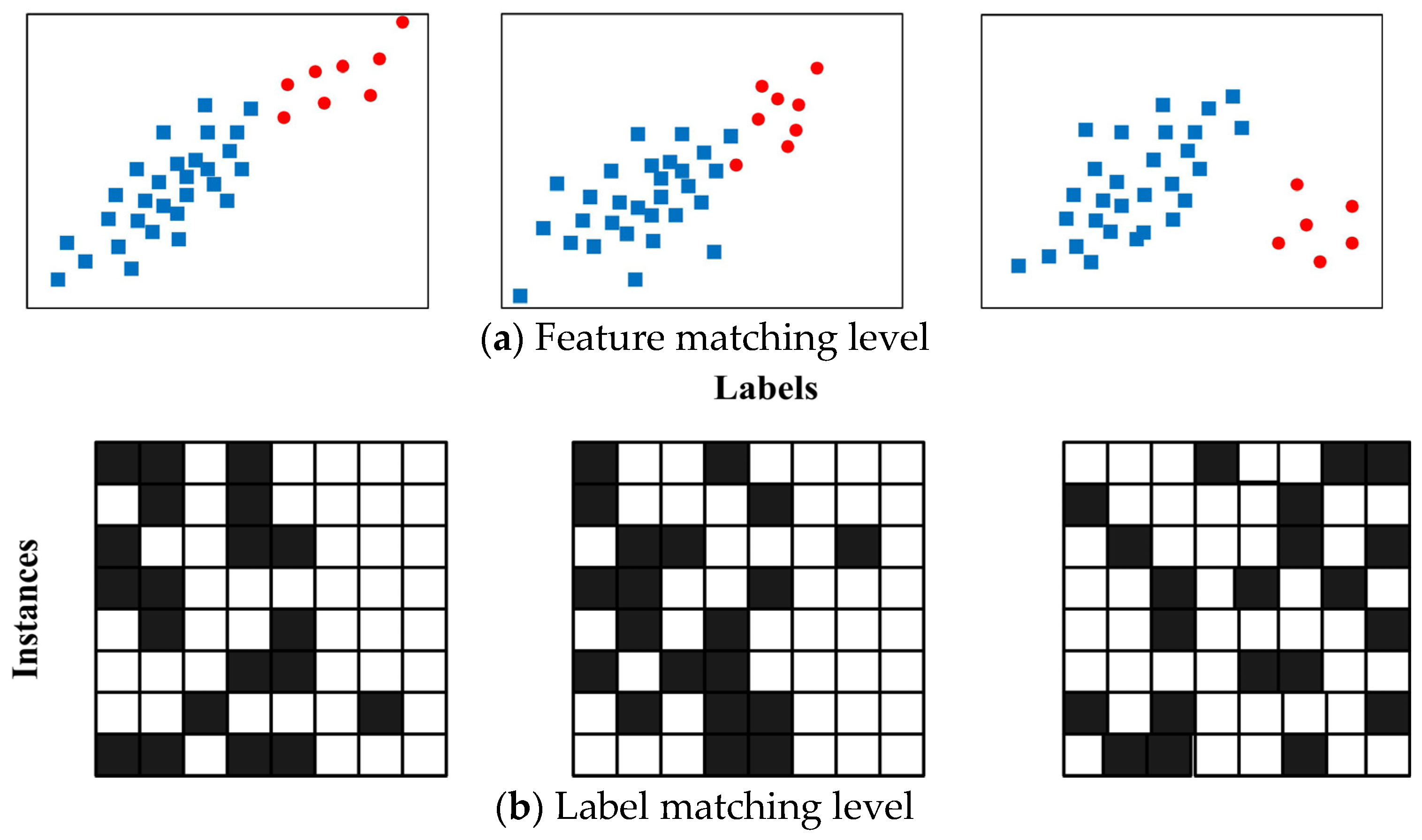Then, it adopts the Kullback–Leibler divergence [24] to detect the feature matching level (feature distribution similarity between two data chunks, see Figure 3a) between each old data chunk and the newest received data chunk. Furthermore, it takes advantage of the feedback feature matching level to adaptively assign decision weights for each corresponding learner in the ensemble. Specifically, DME can provide a just-in-time decision, as it adequately takes advantage of the feature distribution of the newly arrived data chunk and its similarity with that of each reserved old data chunk. In this study, we extended DME to a multi-label data stream. In particular, in addition to the feature matching level, we also consider the degree of the label distribution alteration, i.e., label matching level (label distribution similarity between two data chunks, see Figure 3b), using a label distribution drift detector (LD3) [21]. That is to say, in our algorithm, the weight is adaptively allocated for each base learner in the ensemble by simultaneously considering the feature matching level and label matching level between each reserved data chunk and newly received data chunk. This amendment satisfies the requirement of a just-in-time classification of a nonstationary multi-label data stream. Additionally, in comparison with DME, the proposed MLDME adds a weight allocation threshold to avoid that of those base learners, which are trained on data chunks having a very low distribution similarity with the new data chunk, to participate in decision making. Furthermore, to avoid the infinite extension of ensemble classifiers, we still used a fixed-size buffer to store them and designed three different dynamic classifier updating rules. We conducted experiments on nine artificial and three real-world multi-label nonstationary data streams, and compared them with several popular and state-of-the-art online learning paradigms and algorithms, including two specifically designed ones for classifying a nonstationary multi-label data stream. The results indicate the effectiveness and superiority of the proposed algorithm.

The three main contributions of this study are concluded as follows:

(1)

To adapt a multi-label online learning requirement, this study designs a concept drift detector (integrating both DME [22] and LD3 [21]) while simultaneously considering that drifts happen at the feature level and label level;

(2)

To adapt the just-in-time decision requirement, this study considers collecting both data distribution information and pseudo-label information on a newly received unlabeled data chunk, and then adaptively assigns a decision weight for each base learner according the similarity between each old data chunk and the newly received one;

(3)

Three different ensemble update rules are designed for the proposed algorithm to satisfy various drifting types in practical applications.

The rest of the paper is organized as follows: Section 2 summarizes some related work. In Section 3, the proposed method is described in detail. Section 4 provides the experimental details and results, and further gives the analysis. Finally, Section 5 concludes with the findings and contributions of this paper.

2. Related Work

In this section, we review several benchmark and state-of-the-art online learning algorithms related to our proposed work in this study.

Hoeffding Tree (HT) [25] has been used as an incremental classifier for massive data streams. Different from those traditional decision tree algorithms that adopt a given split evaluation function to select best attribute, the HT uses the Hoeffding bound to calculate the number of samples necessary to select the right split node with a user-specified probability. It implements increment learning without the need for storing instances after they have been used. The drawback of the HT lies in that it cannot adapt concept drift, as old and new knowledge are both totally reserved.

In the context of online weighted ensemble learning, dynamic weighted majority (DWM) [26] is a benchmark algorithm. It maintains a buffer of base classifiers to make a decision, and for each base learner, its weight can be continuously decayed when it provides a wrong prediction for a newly received instance. If the weight of a base classifier is lower than a given threshold, then it would be removed from the ensemble buffer. DWM adapts concept drift by both dynamically removing bad classifiers and adding new classifiers trained on new data.

Another popular online weighted ensemble learning algorithm is the accuracy update ensemble (AUE2) [27]. Unlike DWM, which is constructed in the scenario of one-by-one instance receiving, it assumes that we received new data in form of a data chunk. After a new data chunk has been labeled, AUE2 lets each reserved classifier provide a prediction on that data chunk and acquires the corresponding error rates. Then, it updates the weight of each classifiers by the feedback of error rates. Specifically, in each round, the classifier with the least accuracy would be replaced by the one trained on the new data chunk, while the new added classifier would be given the largest weight, as it is generally regarded as ‘perfect’ classifier based on the underlying hypothesis that each data block always has the most approximate distribution with that close to it. In addition, AUE2 differs from DWM, as it makes each base classifier incrementally learn from the newly received data chunk, which can be well-suited to concept drift.

We note that most emerging online weighted ensemble learning algorithms are based on the basic underlying hypothesis that each data block always has the most approximate distribution with that emerging after it. It is obviously wrong when concept drift happens between two adjacent data chunks. That means when concept drift happens, most ensemble learning algorithms could only provide a delayed decision. Assuming that a ‘perfect’ classifier exists in the ensemble buffer, it could not be assigned a higher weight to provide a prediction for the newly received unlabeled data block. To solve this issue, in our recent work, an algorithm called distribution matching ensemble (DME) [22] was proposed to provide an adaptive and just-in-time prediction for the data stream. Specifically, DME assumes that if two data blocks have an approximate distribution in feature space, then they would hold similar experience on concept prediction. Therefore, we make DME use a Gaussian mixture model (GMM) [23] to accurately measure the data distribution of each received data chunk and the Kullback–Leibler (KL) divergence [24] to detect the feature matching level between each old data chunk and the newest received data chunk. Furthermore, we take advantage of the feedback feature matching level to adaptively assign a decision weight for each corresponding classifier in the ensemble. It not only abides by the one pass rule, as only the GMM parameters of each data chunk in the ensemble are reserved, but also satisfies the requirement of a just-in-time adaptive prediction, since the experience of the newly received data block is used.

As for learning from a multi-label data stream, it will be more complex than learning from a single-label data stream, as concept drift has been re-defined. As we know, multi-label data frequently exist in real-world applications, and in such scenarios, the label correlation should be focused [28,29,30,31]. That means that even if two data blocks have very approximate feature distributions, concept drift would still happen if they have vastly different label correlation distributions [21]. Roseberry and Cano [32] proposed a punitive k nearest neighbors algorithm with a self-adjusting memory (MLSAMP) to classify drifting multi-label data streams. It maintains a sliding window to reserve recent instances and uses the traditional majority-voting KNN classifier in the window to provide a prediction for the newly received instance. Specifically, it also develops a variable window size technique to adapt to various concept drifts, i.e., maintaining a large window when incremental or gradual drifts exist, and a small window if a sudden drift has been detected. In addition, a punitive removal mechanism is designed to immediately remove those instances that have contributed to errors in the window. The MLSAMP algorithm has low time complexity and good adaption for various potential concept drifts. In [33], the authors focused on the negative impact of using a fixed k value for MLSAMP, and hence proposed an improved algorithm called multi-label self-adjusting k nearest neighbors algorithm (MLSA). It adds a label-specific adaptive k module to MLSAMP to adaptively assign an optimal k value for each label in decision making.

It is clear that although several online multi-label learning algorithms for classifying drifting data streams have been developed, they always focused on the scenario of one-by-one instance receiving but ignored the scenario with chunk-by-chunk. In addition, they customarily used a single model with an adaptive forgetting mechanism, but neglected the more flexible and accurate ensemble learning model. Therefore, in this study, we present a more effective and efficient algorithm for adapting chunk-by-chunk multi-label drifting streams.

3. Methods

In this section, we first briefly give the preliminary knowledge related to this study, including the types of concept drift and the basic paradigm of online weighted ensemble learning. Then, we describe how to measure the similarity matching level between two multi-label data blocks in feature space and label space. Finally, we describe the flow path of MLDME algorithm and discuss its time complexity.

3.1. Preliminary Knowledge

3.1.1. Types of Concept Drift

According to the opinions of Webb et al. [3], concept drift is very complex because it not only associates with the variations of feature space, label distribution, and their dependencies but also relates to the variation frequency with time. Suppose $P_t\left(X,Y\right)$ denotes the joint distribution of the received data block $B_t$, where $X=\{x_i|x_i\in {\mathrm{R}}^d,i=\mathrm{1,2},\dots ,N\}$, in which $d$ represents the dimension of the feature space and N represents the number of instances in $B_t$, and $Y=\{y_i|y_i\in \left\{\mathrm{1,2},\dots ,C\right\},i=\mathrm{1,2},\dots ,N\}$, in which C represents the number of classes. If after a time increment $∆$, we observe $P_t\left(X,Y\right)\ne P_{t+∆}\left(X,Y\right)$, then it means that concept drift has happened. The drift may be incurred by $P_t\left(X\right)\ne P_{t+∆}\left(X\right)$, $P_t\left(Y\right)\ne P_{t+∆}\left(Y\right)$, or $P_t\left(Y|X\right)\ne P_{t+∆}\left(Y|X\right)$. 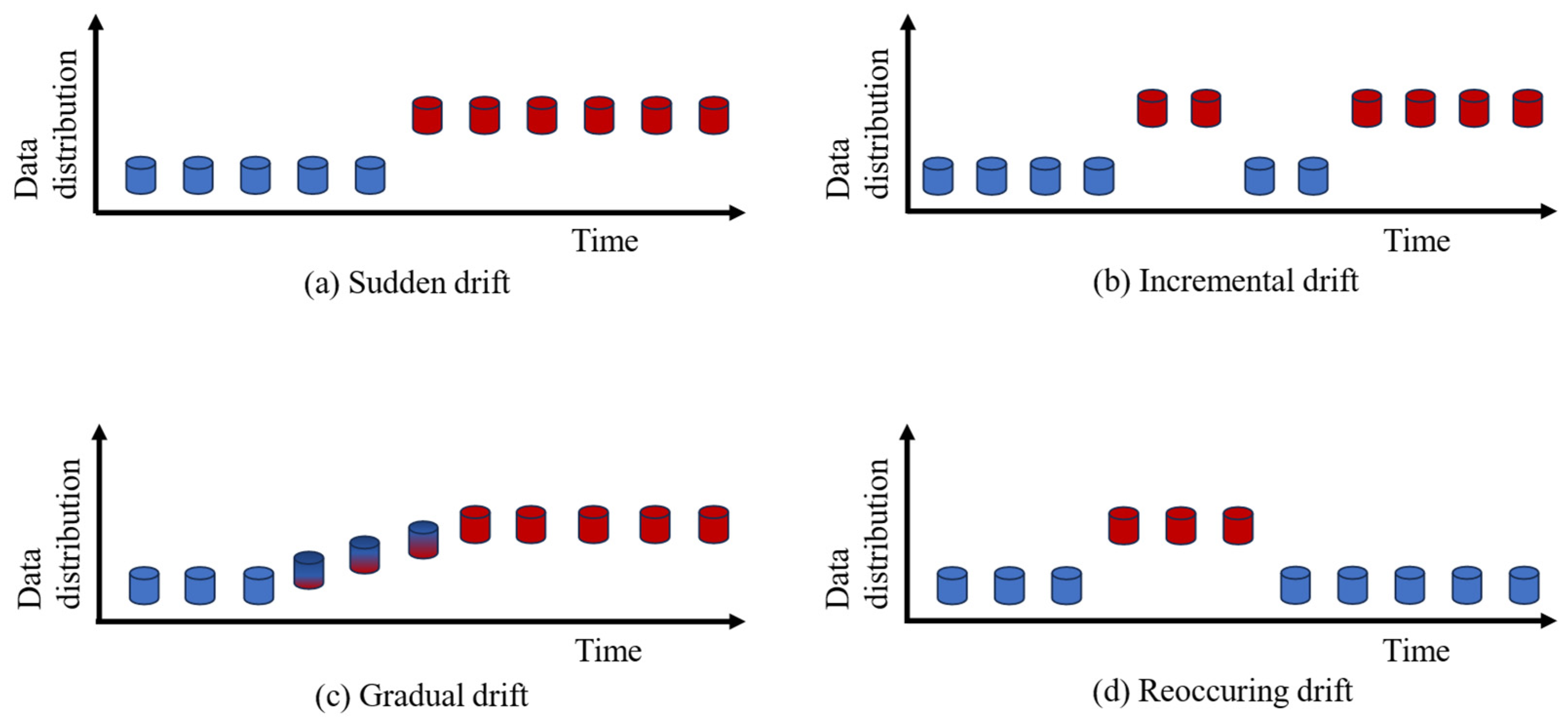Based on the time increment $∆$ and the difference level between two distributions, concept drift can be divided into four types (see Figure 4) as follows:

Sudden drift generally corresponds to a large difference between two continuously received data blocks, i.e., $P_t\left(X,Y\right)\ne P_{t+1}\left(X,Y\right)$, and then the distribution tends to be stable for the next received data block;

Incremental drift generally denotes that the data frequently vibrate between the old distribution and new distribution in a long period, and then it tends to be stable in the form of the new data distribution;

Gradual drift conducts a slight distribution variation of the old data distribution and is gradually changed to be a new data distribution, and then it becomes stable in the form of the new data distribution;

Reoccurring drift suddenly becomes the new data distribution from the old distribution, and then after several or some data blocks, it will become the old distribution again, which means that the drift happens repeatedly.

3.1.2. The Basic Framework of Online Weighted Ensemble Learning

As indicated in Section 1, for nonstationary data streams, online weighted ensemble learning is a more flexible and robust paradigm than an incremental single learning model with a forgetting mechanism. Therefore, in this study, we consider the use of online weighted ensemble learning for dealing with drifting multi-label data streams.

Suppose $\{B_1,B_2,\dots ,B_t,\dots \}$ is an endless multi-label data stream, where $B_t$ denotes the data block received at time $t$. Each data block generally contains an equal number of instances, i.e., $B_t=\left\{\right(x_i,Y_i)|i=\mathrm{1,2},\dots ,N\}$, where $x_i$ denotes the feature vector of the ith instance in $B_t$, $Y_i=\{y_{i1},\dots ,y_{ij},\dots ,y_{i|L|}\}$, $y_{ij}\in \left\{\mathrm{0,1}\right\}$,$|L|$ denotes the number of labels, and $N$ represents the number of instances in a data block. For an online data stream, it is generally supposed that when a data block $B_t$ is just received, its label set is unknown; when and only when the next data block $B_{t+1}$ is received, the real label set for $B_t$ can be obtained.

In the online weighted ensemble learning framework, a fixed-size ensemble buffer is generally maintained to restore some base classifiers $\aleph =\{C_1,C_2,\dots ,C_M\}$, where $C_i$ represents the classifier trained on a data block and $M$ denotes the size of the ensemble buffer. When a new data block $B_t$ is received, it can be predicted by ${\widehat{Y}}_t=w_1{C}_1\left(X_t\right)+\dots +w_M{C}_M\left(X_t\right))$, where $X_t$ and ${\widehat{Y}}_t$, respectively, denote the feature vector and predicted labels of $B_t$, and {$w_1,\dots ,w_M$} represents the decision weight corresponding to each classifier in $\aleph$. In general, the weights are adaptively assigned based on the illustration of each classifier for the data chunk $B_{t-1}$, such as DWM [26] and AUE2 [27], or their illustrations on the data chunk $B_t$, e.g., DME [22]. Then, when the new data chunk $B_{t+1}$ arrives, the new classifier trained on $B_t$ will be added to $\aleph$, and an old classifier in $\aleph$ will be removed based on a preset rule. Next, a new iteration begins.

3.2. Feature Matching Level

As indicated above, data drift may happen in a variety of forms, i.e., $P_t\left(X,Y\right)\ne P_{t+∆}\left(X,Y\right)$ may be incurred by $P_t\left(X\right)\ne P_{t+∆}\left(X\right)$, $P_t\left(Y\right)\ne P_{t+∆}\left(Y\right)$, or $P_t\left(Y|X\right)\ne P_{t+∆}\left(Y|X\right)$. To provide just-in-time adaptive weighting, it is necessary to first detect the feature matching level between any old data chunk and the newly received data chunk. Here, we inherit from the idea of DME [22] to use GMM [23] to extract the distribution information from each data chunk and KL divergence [24] to detect the feature matching level between two data chunks.

GMM [23] has been widely used as to estimate the probability density function (pdf) for any kind of data distribution. In order to approximate any distribution, GMM generally assumes that a unknown probability density function constitutes of $s$ known Gaussian pdfs, and it can be calculated as the weighted sum of these pdfs, i.e.,

$$f\left(\mathbf{x}\right)={\sum }_{i=1}^s{\lambda }_i{f}_i\left(\mathbf{x}\right)={\sum }_{i=1}^s{\lambda }_{i}N\left(\mathbf{x};{\mu }_i,{\mathsf{\Sigma }}_i\right)$$

(1)

where $\lambda$ represents the weight of each Gaussian pdf, and meanwhile, ${\sum }_{i=1}^s{\lambda }_i=1$. $N\left(\mathbf{x};{\mu }_i,{\mathsf{\Sigma }}_i\right)$ corresponds to a Gaussian pdf in $\mathbf{x}$ with the mean vector ${\mu }_i$ and covariance matrix ${\mathsf{\Sigma }}_i$. Specifically, the EM algorithm is generally used to iteratively estimate those parameters existing in GMM. At the E stage, we generally assign $N$ examples to each cluster $i$, and then calculate the probability of a sample $\mathbf{x}$ emerging in that cluster by Equation (2). Next, we assign the example to the cluster which has provided the highest probability.

$${\xi }_i={\displaystyle \frac{{\lambda }_{i}N\left(\mathbf{x};{\mu }_i,{\mathsf{\Sigma }}_i\right)}{{\sum }_{i=1}^s{\lambda }_{i}N\left(\mathbf{x};{\mu }_i,{\mathsf{\Sigma }}_i\right)}}$$

(2)

At the M stage, the following equations are used to model a mixture pdf:

$${\mu }_i={\displaystyle \frac{{\sum }_{j=1}^N\left({\xi }_{ij}{x}_j\right)}{{\sum }_{j=1}^N{\xi }_{ij}}}$$

(3)

$${\mathsf{\Sigma }}_i={\displaystyle \frac{{\sum }_{j=1}^N{\xi }_{ij}\left(x_j-{\mu }_i\right){\left(x_j-{\mu }_i\right)}^{\mathrm{T}}}{{\sum }_{j=1}^N{\xi }_{ij}}}$$

(4)

$${\lambda }_i={\displaystyle \frac{{\sum }_{j=1}^N{\xi }_{ij}}{N}}$$

(5)

Specifically, when we designate a suitable $s$, GMM can accurately approximate any distribution in theory.

As for KL divergence, it is always used to estimate the similarity and/or dissimilarity between two pdfs. Considering there are two different pdfs $f$ and $g$ defined on ${\mathbb{R}}^z$, where $z$ denotes the dimension of the observed vectors, their KL divergence is defined as follows:

$$D_{KL}\left(f||g\right)=\int f\left(\mathbf{x}\right)\log {\displaystyle \frac{f\left(\mathbf{x}\right)}{g\left(\mathbf{x}\right)}}d\mathbf{x}$$

(6)

If both $f$ and $g$ are Gaussian pdfs, then the KL divergence has a closed-form expression described as follows:

$$D_{KL}\left(f||g\right)={\displaystyle \frac{1}{2}}\left(\log {\displaystyle \frac{\left|{\sum }_g\right|}{\left|{\sum }_f\right|}}+\mathrm{T}\mathrm{r}\left({\left({\sum }_g\right)}^{-1}{\sum }_f\right)+{\left({\mu }_f-{\mu }_g\right)}^{\mathrm{T}}{\left({\sum }_g\right)}^{-1}\left({\mu }_f-{\mu }_g\right)-{\displaystyle \frac{d}{2}}\right)$$

(7)

However, for GMM pdfs, there is no a closed-form expression. In such a case, the KL divergence can be approximated to be other functions that may be calculated efficiently. In this study, we adopted the variational approximation strategy proposed by Hershey and Olsen [34] to address this problem.

Let $L_f\left(g\right)=E_X\left[\log g\left(X\right)\right]$, where $X~f$. The KL divergence can be replaced by a decomposition as follows:

$$D_{KL}\left(f||g\right)=L_f\left(f\right)-L_f\left(g\right)$$

(8)

Then the lower bounds for $L_f\left(f\right)$ and $L_f\left(g\right)$ can be obtained using Jensen’s inequality:

$$L_f\left(g\right)\ge {\sum }_a{\lambda }_a^f\log {\sum }_b{\lambda }_b^g{e}^{-D_{KL}\left(f_a||g_b\right)}-{\sum }_a{\lambda }_a^{f}H\left(f_a\right)$$

(9)

$$L_f\left(f\right)\ge {\sum }_a{\lambda }_a^f\log {\sum }_{a^{\prime }}{\lambda }_{a^{\prime }}^f{e}^{-D_{KL}\left(f_a||f_{a^{\prime }}\right)}-{\sum }_a{\lambda }_a^{f}H\left(f_a\right)$$

(10)

These lower bounds can be used as approximations for the corresponding quantities, further acquiring the approximation of KL divergence:

$$D_{var}\left(f||g\right)={\sum }_a{\lambda }_a^f\log {\displaystyle \frac{{\sum }_{a^{\prime }}{\lambda }_{a^{\prime }}^f{e}^{-D\left(f_a||f_{a^{\prime }}\right)}}{{\sum }_b{\lambda }_b^g{e}^{-D\left(f_a||f_b\right)}}}$$

(11)

However, the KL divergence is asymmetric, which means that $D_{var}\left(f||g\right)\ne D_{var}\left(g||f\right)$. To address this issue, it can be transformed to be a Jensen–Shannon (JS) divergence [35], which can be calculated as follows:

$$JSD\left(f||g\right)={\displaystyle \frac{1}{2}}{D}_{var}\left(f||Q\right)+{\displaystyle \frac{1}{2}}{D}_{var}\left(g||Q\right)$$

(12)

where $Q={\displaystyle \frac{f+g}{2}}$ denotes the medium distribution between f and g. It is clear that $JSD\left(f||g\right)\in [0,1]$, and a larger $JSD$ corresponds to a smaller similarity between two data distributions. In other words, JS divergence is a symmetric similarity metric that can provide a stable measure for similarity between two different distributions.

3.3. Label Matching Level

As we know, the feature matching level only detects the similarity between $P_t\left(X\right)$ and $P_{t+∆}\left(X\right)$, which cannot perfectly estimate whether concept drift has occurred. Specifically, in multi-label data streams, the variation in label dependency can be also seen as concept drift. In this study, we use the LD3 (label dependency drift detector) [21] to calculate the label matching level between two data chunks existing in a multi-label data stream. The result of LD3 can partially reflect the similarity between $P_t\left(Y\right)$ and $P_{t+∆}\left(Y\right)$.

In LD3, each data block generates a co-occurrence matrix that is obtained by counting the number of times each class label occurs as “1” alongside other labels. The generated matrix is then ranked within each row, which is called local ranking, by creating a ranking for each label based on their co-occurrence frequencies. After acquiring the local ranking, the ranks can be further aggregated as global ranking as follows:

$$r_i={\displaystyle \frac{1}{{\sum }_{j=1.j\ne i}^{|L|}\frac{1}{r_{ij}}}}$$

(13)

where $r_i$ denotes the ranking score of the label $l_i$, and $r_{ij}$ represents the ranking of the label $l_i$ in the jth row of the local ranking matrix. Next, we obtain the global ranking position sequence R by ranking all $r_i$ in ascending rankings. Suppose $R_p$ and $R_q$, respectively, denote the global ranking sequences of two different data blocks $B_p$ and $B_q$; then, the label matching correlation between these two data blocks can be calculated as follows:

$$Corr=1-{\sum }_{i=1}^{|L|}(2^{-R_{p,i}}·{\displaystyle \frac{|R_{p,i}-R_{q,i}|}{\mathrm{m}\mathrm{a}\mathrm{x}\{\left|1-R_{p,i}\right|,|\left|L\right|-R_{p,i}|\}}})$$

(14)

where $2^{-R_{p,i}}$ denotes the weight of the label $l_i$, which ensures that higher ranking labels have more influence. The numerator $|R_{p,i}-R_{q,i}|$ is the ranking distance of $l_i$ within the two rankings and the denominator scales the distance. It is clear that the higher the Corr is, the more similar the label dependency order between two multi-label data blocks is.

3.4. The Proposed MLDME Algorithm

By integrating the feature matching level and label matching level, it is easy to estimate the similarity between two multi-label data blocks. However, for a newly received unlabeled data chunk, to achieve a just-in-time prediction by taking advantage of prior information, it can directly acquire feature information, while real labels are unknown. In this study, we use the pseudo-labels predicted by each classifier $C_i$ in $\aleph$ to calculate its label dependency order. Although the predicted results may be not accurate, they can still reflect the difference between two data blocks enough.

Suppose $f_i$ denotes the pdf of the data block corresponding to the classifier $C_i$ in the current ensemble buffer $\aleph$, and $g$ denotes the pdf of the newly received data block; then, the feature matching level between these two data blocks can be calculated as follows:

$${simF}_i=1-JSD\left(f_i||g\right)$$

(15)

In addition, suppose $R_i$ denotes the label global ranking sequence of the data block corresponding to the classifier $C_i$, and ${\widehat{R}}_i$ denotes that based on the predicted labels by $C_i$ for the newly received data block; then, the label matching level between these two data blocks can be calculated as follows:

$${simL}_i=1-{\sum }_{j=1}^{|L|}\left(2^{-R_{i,j}}\cdot {\displaystyle \frac{\left|R_{i,j}-{\widehat{R}}_{i,j}\right|}{\max \left\{\left|1-R_{i,j}\right|,\left|n-{\widehat{R}}_{i,j}\right|\right\}}}\right)$$

(16)

Next, the similarity level between two data blocks can be further integrated as follows:

$${simFL}_i=\gamma {simF}_i+(1-\gamma ){simL}_i$$

(17)

where $\gamma$ denotes a regulatory factor to tune the relative significance between the feature level and label level. In this study, $\gamma$ has been empirically designated as 0.5, i.e., the feature level has an equal significance to label level.

Moreover, the voting weight of each classifier $C_i$ can be calculated by its similarity level. Specifically, to avoid the classifiers constructed on the data blocks having significant differences with the newly received data block to participate, a threshold $\tau$ is predesignated. If ${simFL}_i<\tau$, then the classifier $C_i$ is removed from the prediction. That means that for each newly received data chunk, only $M\prime$ classifiers are assigned weights for conducting the ensemble prediction, where $M\prime \le M$. In this study, $\tau$ is empirically set to be 0.2. The weight of each classifier participating in the ensemble decision can be calculated as follows:

$$w_i={\displaystyle \frac{{simFL}_i}{{\sum }_{j=1}^{M^{\prime }}{simFL}_j}}$$

(18)

It is clear that a reserved data chunk has more similar feature and label distributions with the newly received data chunk, and it contributes more to the prediction. In addition, to avoid a decision deficiency when the similarity level of each reserved data chunk with the newly received one is lower than $\tau$, e.g., a sudden drift happens in the new data chunk, we designate the classifier corresponding to the highest similarity to provide a prediction in such a scenario.

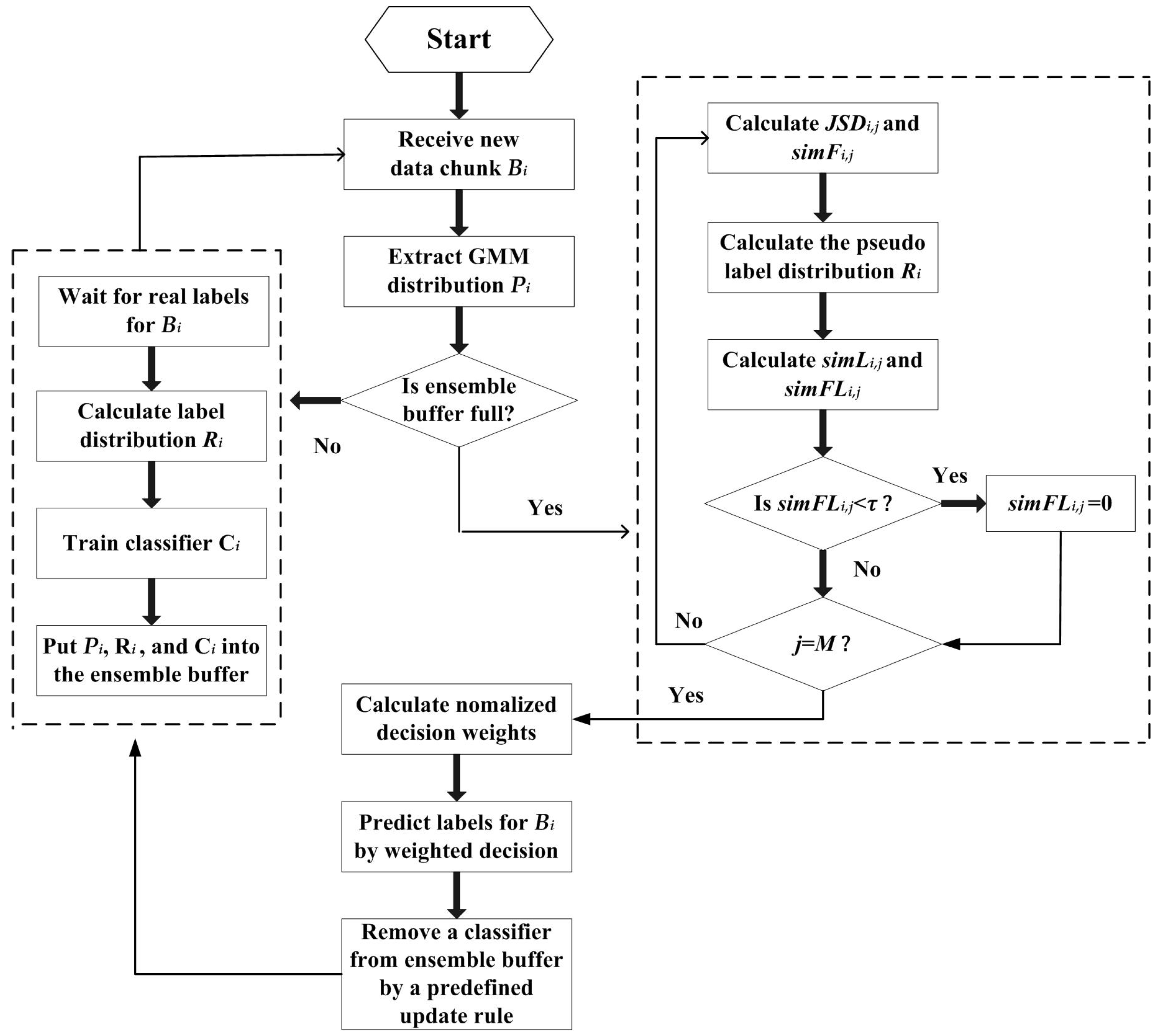
The procedure of the proposed MLDME is described as follows (Algorithm 1):

Algorithm 1 MLDME

Input: a multi-label chunk-based data stream $\{B_1,B_2,\dots \}$ in which each data chunk has n instances and |L| labels, the number of GMM is $s$, the regulatory factor is $\gamma$, the decision threshold is $\tau$, and the size of the ensemble buffer is M

Output: $\aleph =\left\{C_1,C_2,\dots ,C_M\right\}$ with the label distribution information $P_i$ and label global ranking sequence $R_i$ of each corresponding data block

Procedure:

1. $\aleph =\varnothing$;

2. While new data chunk $B_i$ is received

3.   If $\aleph =\varnothing$

4.    Wait real labels of the data chunk $B_i$;

5.    Extract GMM distribution information $P_i$;

6.    Calculate label global ranking sequence $R_i$;

7.    Train a classifier $C_i$ on $B_i$;

8.    Put $C_i$, $P_i,$ and $R_i$ into $\aleph$;

9.   else

10.    For j = 1 to |$\aleph$|

11.     Extract GMM distribution information $P_i$;

12.     Calculate ${JSD}_{i,j}$ by Equation (12);

13.     Calculate ${simF}_{i,j}$ by Equation (15);

14.     Predict pseudo-labels for $B_i$ by $C_j$;

15.     Calculate label global ranking sequence $R_i$ by pseudo-labels;

16.     Calculate ${simL}_{i,j}$ by Equation (16);

17.     Calculate ${simFL}_{i,j}$ by Equation (17);

18.     If ${simFL}_{i,j}$<$\tau$

19.      ${simFL}_{i,j}=0$;

20.     End If

21.    End For

22.    Calculate decision weight for each classifier in $\aleph$ by Equation (18);

23.    Provide prediction for $B_i$ by weighted ensemble voting;

24.    If |$\aleph$|=M

25.     Remove a classifier in $\aleph$ by a pre-setting ensemble update rule;

26.    End IF

27.    Wait real labels of the data chunk $B_i$;

28.    Train a classifier $C_i$ on $B_i$;

29.    Put $C_i$, $P_i,$ and $R_i$ into $\aleph$;

30.   End If

31. End While

In the algorithm description, we note that when the first data chunk is received, it lacks prior knowledge to a provide prediction for it, and hence the first data chunk cannot be predicted, but needs to wait for its real label set. In addition, when and only when the ensemble buffer is full, the classifier update rule is used to replace the most useless classifier by the newly trained one. Here, we designed three different ensemble update rules. First follows the FIFO principle to replace the earliest constructed classifier in $\aleph$ with the new one. AVE maintains a score for each classifier, which uses the decision threshold $\tau$ to calculate the ratio between the participating ensemble decision and undergoing data chunks of that classifier. Certainly, the score is also compulsively decayed with time. This rule reflects the significance of each classifier in the ensemble, and always selects to remove the most useless one. Rec modifies the AVE rule, and it only finds the lowest AVE classifier from the most half oldest ones in the ensemble to guarantee that those newly added classifiers can be reserved longer. It can be seen as a trade-off between two first rules. In this study, we used Rec as the default updating rule. Regarding the performance difference among these three rules, we will discuss it in Section 4. To further clarify the algorithm procedure, a flow chart of the MLDME algorithm is presented in Figure 5.

Since MLDME only reserves M GMM distribution information, label global ranking sequences, and classifiers, it satisfies the one pass requirement of online learning. However, due to the participation of the complex calculation of the feature matching level and label matching level, MLDME has a relatively high time complexity. However, it is acceptable as in real-world applications, as there always exists a longer time interval between two continuous data chunks than that between two continuous instances. The specific running time of various compared algorithms will be given in next section.

4. Experiments

4.1. The Datasets Used in the Experiments

In our experiments, we used three real-world multi-label data sets from a multi-label classification dataset repository that is available at http://www.uco.es/kdis/mllresources/ (accessed on 15 October 2024), and nine synthetic multi-label data streams that cover all drift types.

Among the three real-world datasets, 20 ng collects lots of documents covering 20 different newsgroups, Ohsumed collects medical data associated with 23 different cardiovascular diseases, and Yelp collects a lot of user comments and rates for good or bad evaluations of many services, commodities, transactions, and prices. For these three datasets, each data block except the last one contains 400 instances.

As for synthetic datasets, they are generated by the approach used in [21]. Each synthetic dataset contains 20,000 instances that are averagely assigned into 50 data blocks. That means that each data block holds 400 instances. Reoccur_k denotes the reoccurring drift that happens after every k continuous data blocks. Gradual denotes that the data stream slowly drifts from one distribution to another distribution. Both Increment₁ and Increment₂ simulate the incremental drift, and their distinction lies in that Increment₁ drifts faster than Increment₂. Similarly, both Sudden_s and Sudden_f simulate sudden drift, and they are different, as sudden drift only happens once in Sudden_s, while Sudden_f activates sudden drift every 10 data blocks.

The detailed information about these datasets is described in

Table 1. Datasets used in this study.

Dataset	#Instances	#Features	#Labels	Label Cardinality
20 ng	19,300	1006	20	1.03
Ohsumed	13,929	1002	23	1.66
Yelp	10,806	671	5	1.64
Reoccur5	20,000	50	10	3.00
Reoccur10	20,000	50	10	2.80
Reoccur15	20,000	50	10	2.80
Reoccur20	20,000	50	10	2.80
Gradual	20,000	50	10	4.26
Suddenf	20,000	50	10	3.65
Suddens	20,000	50	10	3.00
Incremental1	20,000	50	10	3.60
Incremental2	20,000	50	10	3.62

.

4.2. Experimental Settings

In the experiments, we compared the proposed MLDME algorithm with several popular and state-of-the-art algorithms, including HT [25], DWM [26], AUE2 [27], DME [22], MLSAMP [32], and MLSA [33]. The experiments were performed using Scikit-Multiflow [36]. Specifically, DWM, AUE2, DME, and MLDME share the common parameter $M=10$, and DME and MLDME share the common number of GMM $s=5$. For MLSAM and MLSA, the size of maximum window is designated as 1200. As for the classification algorithm, we designated extreme learning machine (ELM) [37,38] as the base learning algorithm, where the number of hidden-layer nodes has been empirically set to be 100 and the penalty factor has been set to be 10.

We adopted four popular multi-label learning performance evaluation metrics to compare various algorithms. They are Subset Accuracy, Hamming Score, Macro-averaged F1, and Micro-averaged F1, respectively. Suppose there are N testing instances; $Y_i$ ($i\in \{\mathrm{1,2},\dots ,N\}$) represents the real labels of the ith instance, and ${\widehat{Y}}_i$ ($i\in \{\mathrm{1,2},\dots ,N\}$) denotes the predicted labels of that instance. Then, Subset Accuracy can be calculated as follows:

$$\mathrm{Subset}\mathrm{Accuracy}={\displaystyle \frac{1}{N}}{\sum }_{i=0}^{N}1|Y_i={\widehat{Y}}_i$$

(19)

The Hamming Score can be calculated as follows:

$$\mathrm{Hamming}\mathrm{Score}={\displaystyle \frac{1}{N|L|}}{\sum }_{i=0}^N{\sum }_{j=0}^{|L|}1|y_{ij}={\widehat{y}}_{ij}$$

(20)

where $y_{ij}$ and ${\widehat{y}}_{ij}$ denote the real and predicted jth label of the ith instance. It is clear that the Subset Accuracy corresponds to the ratio between the number of testing instances that have been accurately predicted throughout all labels and the total number of testing instances, while the $\mathrm{Hamming}\mathrm{Score}$ denotes the ratio between the number of accurately predicted example–label pairs and the total number of example–label pairs. As for the two other metrics, their calculation requires making use of the results of several other metrics, including the number of true positive instances (TP), the number of true negative instances (TN), the number of false positive instances (FP), and the number of false negative instances (FN). They can be calculated as follows:

$${TP}_j={\sum }_{i=0}^{N}1\mid y_{\mathrm{i}\mathrm{j}}={\widehat{y}}_{\mathrm{i}\mathrm{j}}=1$$

(21)

$${TN}_j={\sum }_{i=0}^{N}1\mid y_{\mathrm{i}\mathrm{j}}={0,\widehat{y}}_{\mathrm{i}\mathrm{j}}=0$$

(22)

$${FP}_j={\sum }_{i=0}^{N}1\mid y_{\mathrm{i}\mathrm{j}}={0,\widehat{y}}_{\mathrm{i}\mathrm{j}}=1$$

(23)

$${FN}_j={\sum }_{i=0}^{N}1\mid y_{\mathrm{i}\mathrm{j}}={1,\widehat{y}}_{\mathrm{i}\mathrm{j}}=0$$

(24)

Specifically, ${TP}_j$ and ${TN}_j$, respectively, record the number of instances whose real and predicted labels are both positive and negative on the jth label, while ${FP}_j$ and ${FN}_j$ record the number of instances that belong to the negative (positive) class but have been predicted as belonging to the positive (negative) class for that label, respectively. Furthermore, they can be used to calculate several evaluation metrics as follows:

$$\mathrm{Macro}-\mathrm{Precision}={\displaystyle \frac{1}{|L|}}{\sum }_{j=1}^{|L|}{\displaystyle \frac{{TP}_j}{{TP}_j+{FP}_j}}$$

(25)

$$\mathrm{Macro}-\mathrm{Recall}={\displaystyle \frac{1}{|L|}}{\sum }_{j=1}^{|L|}{\displaystyle \frac{{TP}_j}{{TP}_j+{FN}_j}}$$

(26)

$$\mathrm{M}\mathrm{i}\mathrm{cro}-\mathrm{Precision}={\displaystyle \frac{{\sum }_{j=1}^{|L|}{TP}_j}{{\sum }_{j=1}^{|L|}{TP}_j+{\sum }_{j=1}^{|L|}{FP}_j}}$$

(27)

$$\mathrm{M}\mathrm{i}\mathrm{cro}-\mathrm{Recall}={\displaystyle \frac{{\sum }_{j=1}^{|L|}{TP}_j}{{\sum }_{j=1}^{|L|}{TP}_j+{\sum }_{j=1}^{|L|}{FN}_j}}$$

(28)

Specifically, Precision and Recall calculate the accuracy of instances that have been predicted as the positive class and accurately predicted as the positive class, respectively. The difference between Macro and Micro lies in that the former first calculates the performance on each label and then calculates the average performance, while the latter one directly calculates the performance throughout all labels. Further, Macro-averaged F1 and Micro-averaged F1 can be calculated as follows:

$$\mathrm{M}\mathrm{a}\mathrm{c}\mathrm{r}\mathrm{o}-\mathrm{a}\mathrm{v}\mathrm{e}\mathrm{r}\mathrm{a}\mathrm{g}\mathrm{e}\mathrm{d} \mathrm{F}1={\displaystyle \frac{2\times \mathrm{Macro}-\mathrm{Precision}\times \mathrm{Macro}-\mathrm{Recall}}{\mathrm{Macro}-\mathrm{Precision}+\mathrm{Macro}-\mathrm{Reca}\mathrm{l}\mathrm{l}}}$$

(29)

$$\mathrm{M}\mathrm{i}\mathrm{c}\mathrm{r}\mathrm{o}-\mathrm{a}\mathrm{v}\mathrm{e}\mathrm{r}\mathrm{a}\mathrm{g}\mathrm{e}\mathrm{d} \mathrm{F}1={\displaystyle \frac{2\times \mathrm{M}\mathrm{i}\mathrm{cro}-\mathrm{Precision}\times \mathrm{M}\mathrm{i}\mathrm{cro}-\mathrm{Recall}}{\mathrm{M}\mathrm{i}\mathrm{cro}-\mathrm{Precision}+\mathrm{M}\mathrm{i}\mathrm{cro}-\mathrm{Reca}\mathrm{l}\mathrm{l}}}$$

(30)

where $\mathrm{M}\mathrm{a}\mathrm{c}\mathrm{r}\mathrm{o}-\mathrm{a}\mathrm{v}\mathrm{e}\mathrm{r}\mathrm{a}\mathrm{g}\mathrm{e}\mathrm{d} \mathrm{F}1$ estimates the tradeoff between $\mathrm{Macro}-\mathrm{Precision}$ and $\mathrm{Macro}-\mathrm{Recall}$, while $\mathrm{M}\mathrm{i}\mathrm{c}\mathrm{r}\mathrm{o}-\mathrm{a}\mathrm{v}\mathrm{e}\mathrm{r}\mathrm{a}\mathrm{g}\mathrm{e}\mathrm{d} \mathrm{F}1$ evaluates the tradeoff between $\mathrm{Micro}-\mathrm{Precision}$ and $\mathrm{Micro}-\mathrm{Recall}$.

Finally, the average predicted performance throughout all data blocks is used to compare the quality of various algorithms.

4.3. Experimental Results

The experimental results are presented in

Table 2. Results of various compared algorithms for the Subset Accuracy metric, in where the best result on each data stream has been highlighted in bold.

Dataset	DME	MLSAMP	MLSA	DWM	HT	AUE2	MLDME
20 ng	0.4218	0.3417	0.3615	0.3655	0.3755	0.3932	0.4234
Ohsumed	0.4803	0.4779	0.4725	0.4756	0.4743	0.4678	0.4804
Yelp	0.3309	0.3079	0.3437	0.2894	0.3022	0.3418	0.3558
Reoccur5	0.5163	0.3072	0.4879	0.0697	0.3148	0.1402	0.5702
Reoccur10	0.3680	0.2616	0.3591	0.1042	0.1977	0.1302	0.3970
Reoccur15	0.4134	0.2769	0.5390	0.2166	0.2741	0.2337	0.4592
Reoccur20	0.3970	0.3252	0.5907	0.1761	0.2536	0.2682	0.4602
Gradual	0.6850	0.7626	0.7208	0.4835	0.5961	0.7044	0.7030
Suddenf	0.0710	0.0471	0.0577	0.0559	0.0749	0.0659	0.0829
Suddens	0.3789	0.3102	0.5424	0.1551	0.3102	0.2010	0.4601
Incremental1	0.8842	0.8900	0.8752	0.2468	0.7644	0.8882	0.8795
Incremental2	0.7933	0.8216	0.7952	0.3495	0.6694	0.8102	0.8229

,

Table 3. Results of various compared algorithms for the Hamming Score metric, in where the best result on each data stream has been highlighted in bold.

Dataset	DME	MLSAMP	MLSA	DWM	HT	AUE2	MLDME
20 ng	0.9471	0.9400	0.9432	0.9407	0.9423	0.9436	0.9474
Ohsumed	0.9658	0.9656	0.9650	0.9655	0.9650	0.9650	0.9660
Yelp	0.8302	0.7808	0.8108	0.8226	0.8225	0.8306	0.8337
Reoccur5	0.8115	0.8053	0.8915	0.7362	0.8750	0.7482	0.8929
Reoccur10	0.8259	0.8512	0.8877	0.7621	0.8488	0.7754	0.8532
Reoccur15	0.9042	0.8181	0.9051	0.7991	0.8670	0.8176	0.9060
Reoccur20	0.8294	0.8323	0.9187	0.7939	0.8683	0.8571	0.9021
Gradual	0.9514	0.9564	0.9555	0.8588	0.9402	0.9546	0.9509
Suddenf	0.6523	0.6874	0.7061	0.6538	0.7116	0.6970	0.6688
Suddens	0.8958	0.8281	0.9059	0.7705	0.8847	0.8292	0.9052
Incremental1	0.9802	0.9767	0.9777	0.8522	0.9648	0.9804	0.9801
Incremental2	0.9657	0.9605	0.9619	0.8334	0.9483	0.9663	0.9713

,

Table 4. Results of various compared algorithms for the Macro-averaged F1 metric, in where the best result on each data stream has been highlighted in bold.

Dataset	DME	MLSAMP	MLSA	DWM	HT	AUE2	MLDME
20 ng	0.0527	0.0895	0.2032	0.0972	0.1033	0.0785	0.0538
Ohsumed	0.0226	0.0205	0.0456	0.0335	0.0256	0.0233	0.0279
Yelp	0.2164	0.2612	0.2647	0.1223	0.1813	0.2619	0.2917
Reoccur5	0.7879	0.6118	0.7766	0.3183	0.7149	0.3057	0.8579
Reoccur10	0.6572	0.5963	0.6976	0.3602	0.5842	0.3572	0.7268
Reoccur15	0.7170	0.5536	0.7443	0.3715	0.6116	0.4428	0.7581
Reoccur20	0.6675	0.5907	0.7824	0.3626	0.5913	0.5589	0.7534
Gradual	0.9411	0.9456	0.9446	0.8407	0.9244	0.9445	0.9402
Suddenf	0.2708	0.3729	0.3532	0.3258	0.3585	0.3635	0.3327
Suddens	0.6694	0.6163	0.7695	0.3266	0.7022	0.4696	0.7299
Incremental1	0.9721	0.9662	0.9689	0.7323	0.9475	0.9726	0.9718
Incremental2	0.9546	0.9494	0.9503	0.7631	0.9129	0.9559	0.9614

and

Table 5. Results of various compared algorithms for the Micro-averaged F1 metric, in where the best result on each data stream has been highlighted in bold.

Dataset	DME	MLSAMP	MLSA	DWM	HT	AUE2	MLDME
20 ng	0.4523	0.2742	0.3710	0.4277	0.4457	0.4478	0.4535
Ohsumed	0.0628	0.0571	0.0852	0.1003	0.0514	0.0739	0.0834
Yelp	0.2787	0.3816	0.3596	0.1658	0.2132	0.3252	0.3479
Reoccur5	0.7911	0.6652	0.7988	0.4425	0.7569	0.4007	0.8701
Reoccur10	0.7186	0.6590	0.7418	0.4798	0.6647	0.4921	0.7682
Reoccur15	0.8283	0.6277	0.7972	0.5756	0.7217	0.6372	0.8362
Reoccur20	0.7619	0.6681	0.8275	0.5808	0.6913	0.7215	0.8327
Gradual	0.9439	0.9489	0.9479	0.8447	0.9301	0.9472	0.9436
Suddenf	0.3574	0.4723	0.4606	0.4026	0.5045	0.4632	0.4222
Suddens	0.8123	0.6809	0.8152	0.5560	0.7695	0.6763	0.8286
Incremental1	0.9743	0.9690	0.9713	0.7807	0.9507	0.9746	0.9741
Incremental2	0.9573	0.9524	0.9534	0.7632	0.9247	0.9585	0.9637

. Specifically, the best result for each dataset has been highlighted in bold. From these results, we can observe several conclusions as follows:

(1)

For each performance evaluation metric except Macro-averaged F1, the proposed MLDME performed better than each of other compared algorithms, indicating its effectiveness and superiority. Specifically, it performed best on seven, six, five, and seven datasets in terms of the Subset Accuracy, Hamming Score, Macro-averaged F1, and Micro-averaged F1, respectively. We believe that it mainly profits from the just-in-time mechanism that takes full advantage of the information acquired from the newly received unlabeled data chunk. The mechanism can make MLDME adapt to concept drift in a timelier manner.

(2)

We also note that in addition to MLDME, both MLSAMP and MLSA have shown more superiority to several other competitors, and their superiority is specifically significant in data streams with gradual and sudden drifts. In our opinion, their superiority comes from the one-by-one processing manner used by them, which make them can adapt faster to suddenly occurring concept drifts.

(3)

Although DME performs worse than MLDME, it significantly outperforms several traditional online weighted ensemble learning algorithms, including HT, DWM, and AUE2, on most data streams. The results illustrate the necessity of making use of the distribution information of the newly received unlabeled data chunk to make a just-in-time decision again. In addition, DME performs worse than MLDME, showing the necessity of considering the label matching level, though some pseudo-labels assigned to the newly received data chunk might be wrong.

(4)

About the different types of concept drift, the proposed MLDME seems to be performing better on reoccurring drift and incremental drift. It is first because of the adoption of both the feature matching level and label matching level. Additionally, it is related to its weight assignment mechanism and classifier updating rule. However, when reoccurring drift happens between a large data block interval, e.g., Reoccur₁₅ and Reoccur₂₀, MLDME tends to be out of work as the ensemble buffer has removed those closely associated classifiers from the data block.

We also presented performance variation curves of various compared algorithms for several representative datasets, including Reoccur₅, Reoccur₁₅, Sudden_s, and 20 ng, in Figure 6, Figure 7, Figure 8 and Figure 9.

The results in Figure 6 and Figure 7 show that when reoccurring drift happens in a small interval, the proposed MLDME algorithm can adaptively provide an excellent prediction for drifting data chunks, but when reoccurring drift happens at a low frequency, the performance of MLDME would be significantly decreased. It is consistent with our analysis above. The solution is enlarging the ensemble buffer to make it comprise prior knowledge in a longer period. The results in Figure 8 illustrate that similar to other online learning algorithms, MLDME cannot immediately adapt to unseen sudden drift, but it can fit the new data distribution faster than HT and DWM through its adaptive weight assignment mechanism. In Figure 9, we observe that MLDME performs well on real-world nonstationary multi-label data streams, and it can rapidly track and adapt data distribution variations. We believe that it profits from making full use of the information of the newly received data chunk, further provides a just-in-time decision, and adaptively responds to data variations.

4.4. Significance Analysis Using Statistics

Furthermore, the Nemenyi test is adopted as a post hoc test for the Friedman test [39,40] to investigate the performance significance of the proposed MLDME algorithm. Here, we focus on the relative performance between our proposed MLDME algorithm and the other compared algorithms. If the average rank of the MLDME and that of a compared algorithm differ by at least one critical difference (CD) unit, then we consider that their performance is significantly different. Specifically, the CD is calculated as follows:

$$CD=q_{\alpha }\sqrt{{\displaystyle \frac{U(U+1)}{6H}}}$$

(31)

where $q_{\alpha }$ denotes the significance level, $U$ indicates the number of compared algorithms in the experiments, and $H$ represents the number of datasets used in the experiments. In a CD diagram, if the average ranks of two algorithms are less than a CD unit, then they would be connected by a thick line to indicate that their difference is not significant at a specific significance level. Figure 10 presents the CD diagrams for four different metrics.

In Figure 10, we observe that MLDME performs best on Subset Accuracy, Hamming Score, and Micro-averaged F1 metrics, and is runner-up on the Macro-averaged F1 metric, indicating its superiority. Specifically, on the Subset Accuracy metric, MLDME significantly outperforms the DWM, HT, and AUE2 algorithms, while in terms of three other performance metrics, MLDME only significantly outperforms the DWM algorithm. Although compared with the majority of algorithms, the superiority of MLDME is not significant enough, it is still best as it has acquired lower average rankings.

4.5. Ablation Experiments

Further ablation experiments were conducted to investigate whether both the feature matching level and label matching level have contributed to the success of MLDME. Specifically, we compared the performance of MLDME when adopting $simFL$, and only using $simF$ and $simL$ as the similarity metric. The results are presented in

Table 6. Results of the ablation experiments, in where the best result on each data stream in terms of each performance metric.

	Subset Accuracy			Hamming Score			Macro-Averaged F1			Micro-Averaged F1
Dataset	simFL	simF	simL	simFL	simF	simL	simFL	simF	simL	simFL	simF	simL
20 ng	0.4234	0.3853	0.4050	0.9474	0.9425	0.9456	0.0538	0.0821	0.0752	0.4535	0.4492	0.4583
Ohsumed	0.4804	0.4603	0.4738	0.9660	0.9641	0.9655	0.0279	0.0515	0.0455	0.0834	0.1600	0.1361
Yelp	0.3558	0.3671	0.4067	0.8337	0.8191	0.8401	0.2917	0.3992	0.3938	0.3479	0.4521	0.4491
Reoccur5	0.5702	0.3901	0.4538	0.8929	0.8592	0.8954	0.8579	0.7444	0.7936	0.8701	0.7710	0.8183
Reoccur10	0.3970	0.3591	0.4211	0.8532	0.7789	0.7729	0.7268	0.5452	0.5333	0.7682	0.5989	0.5872
Reoccur15	0.4592	0.5181	0.5155	0.9060	0.9119	0.9119	0.7581	0.6112	0.6102	0.8362	0.6984	0.6912
Reoccur20	0.4602	0.2813	0.4505	0.9021	0.8375	0.8676	0.7534	0.5453	0.7021	0.8327	0.6960	0.7730
Gradual	0.7030	0.6967	0.6962	0.9509	0.9498	0.9492	0.9402	0.9393	0.9385	0.9436	0.9425	0.9418
Suddenf	0.0829	0.0291	0.0270	0.6688	0.6290	0.6201	0.3327	0.3859	0.3810	0.4222	0.4473	0.4393
Suddens	0.4601	0.2910	0.5114	0.9052	0.8682	0.9100	0.7299	0.5946	0.7813	0.8286	0.7537	0.8445
Incremental1	0.8795	0.7377	0.7297	0.9801	0.9010	0.8960	0.9718	0.8582	0.8519	0.9741	0.8692	0.8625
Incremental2	0.8229	0.8152	0.8160	0.9713	0.9687	0.9689	0.9614	0.9586	0.9588	0.9637	0.9610	0.9612

.

From the results in Table 6, we observe that integrating $simF$ and $simL$, i.e., $simFL$, produced best results for seven, eight, seven, and seven datasets in terms of Subset Accuracy, Hamming Score, Macro-averaged F1, and Micro-averaged F1 metrics, respectively. The results indicate the necessity of integrating these two matching levels to estimate the similarity between two multi-label data chunks. It can provide more comprehensive information than independently considering either the feature level or label level. In addition, an interesting phenomenon is observed, that is, matching the feature level similarity seems to help more in improving the accuracy of an individual instance, while matching the label level similarity helps to promote learning performance in terms of equilibrium.

4.6. Comparison of Three Ensemble Updating Rules

Next, we compared the performance of the three different ensemble updating rules presented in Section 3, i.e., First, Ave, and Rec. The results are presented in

Table 7. Experimental comparison of three ensemble updating rules, in where the best result on each data stream in terms of each performance metric.

	Subset Accuracy			Hamming Score			Macro-Averaged F1			Micro-Averaged F1
Dataset	Rec	Ave	First	Rec	Ave	First	Rec	Ave	First	Rec	Ave	First
20 ng	0.4234	0.3776	0.3873	0.9474	0.9456	0.9465	0.0538	0.0849	0.0791	0.4535	0.4465	0.4450
Ohsumed	0.4804	0.4401	0.4565	0.9660	0.9653	0.9647	0.0279	0.0550	0.0514	0.0834	0.1634	0.1564
Yelp	0.3558	0.2880	0.3222	0.8337	0.8319	0.8279	0.2917	0.3697	0.3896	0.3479	0.4024	0.4207
Reoccur5	0.5702	0.5586	0.6472	0.8929	0.8929	0.9449	0.8579	0.8234	0.8336	0.8701	0.8461	0.8496
Reoccur10	0.3970	0.3756	0.3889	0.8532	0.8466	0.8491	0.7268	0.6882	0.7103	0.7682	0.7329	0.7472
Reoccur15	0.4592	0.4505	0.4472	0.9060	0.9022	0.8967	0.7581	0.7957	0.8027	0.8362	0.8415	0.8394
Reoccur20	0.4602	0.4020	0.4342	0.9021	0.8693	0.8729	0.7534	0.7380	0.6835	0.8327	0.8161	0.7728
Gradual	0.7030	0.6929	0.6959	0.9509	0.9534	0.9544	0.9402	0.9431	0.9441	0.9436	0.9460	0.9471
Suddenf	0.0829	0.0202	0.0224	0.6688	0.5894	0.6151	0.3327	0.3300	0.3804	0.4222	0.3788	0.4378
Suddens	0.4601	0.6022	0.5177	0.9052	0.9248	0.9382	0.7299	0.8702	0.8122	0.8286	0.9006	0.8677
Incremental1	0.8795	0.8276	0.8271	0.9801	0.9475	0.9478	0.9718	0.9202	0.9258	0.9741	0.9288	0.9310
Incremental2	0.8229	0.6793	0.6457	0.9713	0.8899	0.8736	0.9614	0.8143	0.7822	0.9637	0.8186	0.7878

, where we observe that MLDME with Rec rule have produced best results for ten, nine, five, and six datasets in terms of Subset Accuracy, Hamming Score, Macro-averaged F1, and Micro-averaged F1 metrics, respectively. The results illustrate that adopting the Rec rule is significantly better than using two other rules. At least we can say that using the Rec rule is safer than using the other two. It is believed that the Rec rule simultaneously considers the utilization rate and survival time of a classifier in the ensemble buffer, which can save those most useful classifiers to a large extent. While Ave tends to remove those new but potentially useful ones from the ensemble buffer, further resulting in the loss of decision information and performance degeneration. As for the First rule, although it is simple, we note that it can still acquire excellent performance in several specific drifting scenarios, e.g., frequent reoccurring drifts and slow gradual drifts. In practical applications, we recommend to use the Rec ensemble updating rule as a safe setting.

4.7. Comparison of the Running Time

Finally, we compared the running times of various compared algorithms when treating one data chunk, and provided the results in

Table 8. Experimental results for the running time (seconds).

Dataset	DME	MLSAMP	MLSA	DWM	HT	AUE2	MLDME
20 ng	2.72 × 101	5.27 × 10−1	5.16 × 10−1	2.37	3.62 × 10−1	2.52	2.92 × 10−1
Ohsumed	1.92 × 101	5.74 × 10−1	5.64 × 10−1	2.78	3.81 × 10−1	3.03	2.18 × 10−1
Yelp	1.16 × 101	9.62 × 10−1	9.11 × 10−1	1.51	1.53 × 10−1	1.63	1.58 × 10−1
Reoccur5	2.23	3.43 × 10−1	3.52 × 10−1	8.89 × 10−1	1.29 × 10−1	9.02 × 10−1	2.85
Reoccur10	2.45	3.51 × 10−1	3.44 × 10−1	7.89 × 10−1	1.32 × 10−1	8.22 × 10−1	2.86
Reoccur15	3.36	3.64 × 10−1	3.55 × 10−1	7.35 × 10−1	1.40 × 10−1	8.02 × 10−1	2.57
Reoccur20	3.12	1.19 × 10−1	3.64 × 10−1	8.29 × 10−1	1.39 × 10−1	7.81 × 10−1	4.20
Gradual	1.59	3.63 × 10−1	3.51 × 10−1	8.98 × 10−1	1.34 × 10−1	8.85 × 10−1	2.07
Suddenf	4.18	3.94 × 10−1	3.86 × 10−1	7.36 × 10−1	1.34 × 10−1	7.51 × 10−1	5.80
Suddens	1.90	3.65 × 10−1	3.59 × 10−1	6.97 × 10−1	1.41 × 10−1	7.17 × 10−1	1.99
Incremental1	0.91	3.62 × 10−1	3.85 × 10−1	8.99 × 10−1	2.38 × 10−1	7.81 × 10−1	1.04
Incremental2	0.80	3.07 × 10−1	3.19 × 10−1	8.97 × 10−1	2.43 × 10−1	8.77 × 10−1	1.03

. We observed that both DME and MLDME are obviously more time-consuming than several other compared algorithms throughout almost all data streams. For DME, we believe that most of its running time costs occur when calculating the GMM for the new data chunk and the KL divergence between M block pairs. As for MLDME, it spends more time estimating the label distribution and calculating the label matching level between any one reserved data chunk and the newly received data chunk. As indicated in Section 3, although MLDME is much more time-consuming than those simple algorithms, it is still acceptable as in real-world applications, as there always exists a long time interval between two continuous data chunks.

5. Conclusions

In this study, an adaptive and just-in-time online weighted ensemble multi-label learning algorithm called MLDME is proposed. It synchronously focuses on the feature distribution and pseudo-label distribution of a newly received unlabeled data chunk according to the similarities with that of labeled historic data chunks to adaptively assign a decision weight for each corresponding classifier. Specifically, MLDME adopts JS divergence based on a Gaussian mixture model to estimate feature distribution similarity and the LD3 approach to calculate the label distribution similarity between two data blocks. In addition, three different ensemble updating rules are proposed. The experimental results for nine synthetic multi-label data streams and three real-world data streams indicate the necessity of taking full advantage of the newly received unlabeled data chunk, which can effectively avoid a decision delay. In addition, the results show that MLDME outperforms several traditional online weighted ensemble learning paradigms and state-of-the-art multi-label online learning algorithms.

Future work intends to modify MLDME to make it adapt to the streaming scenario with receiving instances one-by-one. Additionally, how to dynamically and adaptively call the ensemble updating rule according to the feedback of distribution matching information will be investigated too.