Deep Multi-View Clustering Optimized by Long Short-Term Memory Network

Abstract

Long short-term memory (LSTM) networks have shown great promise in sequential data analysis, especially in time-series and natural language processing. However, their potential for multi-view clustering has been largely underexplored. In this paper, we introduce a novel approach called deep multi-view clustering optimized by long short-term memory network (DMVC-LSTM), which leverages the sequential modeling capability of LSTM to effectively integrate multi-view data. By capturing complex interdependencies and nonlinear relationships between views, DMVC-LSTM improves clustering accuracy and robustness. The method includes three feature fusion techniques—concatenation, averaging, and attention-based fusion—with concatenation as the primary method. Notably, DMVC-LSTM is well suited for datasets that exhibit symmetry, as it can effectively handle symmetrical relationships between views while preserving the underlying structures. Extensive experiments demonstrate that DMVC-LSTM outperforms existing multi-view clustering algorithms, particularly in high-dimensional and complex datasets, achieving superior performance in datasets like 20 Newsgroups and Wikipedia Articles. This paper presents the first application of LSTM in multi-view clustering, marking a significant step forward in both clustering performance and the application of LSTM in multi-view data analysis.

1. Introduction

With the rapid growth in multi-view data, where the same object or event is described from multiple perspectives, multi-view clustering has become an essential tool for uncovering the underlying structure of such data [1]. These types of data often contain complementary and interdependent information across views, and effectively integrating these views can improve the performance of clustering tasks [2,3]. Multi-view clustering aims to partition data by leveraging the information from all views, thus revealing the inherent symmetries within the data structure [4].

Traditional single-view clustering methods, such as k-means [5] and spectral clustering [6], struggle when dealing with complex, high-dimensional, and heterogeneous datasets. These methods are limited to processing data from a single perspective and fail to capture the full complexity of multi-view data [7]. Multi-view clustering, on the other hand, has been introduced to overcome this limitation by combining information from different views, resulting in more robust and accurate clustering performance [8,9]. However, existing multi-view clustering approaches still face significant challenges, including information redundancy, ineffective view weight allocation, and the inability to capture complex nonlinear relationships between views [10,11].

In recent years, deep learning has led to breakthroughs in multi-view clustering. Deep learning models can automatically learn feature representations from raw data, thus eliminating the need for manual feature extraction [12]. Several deep models, including autoencoders and deep neural networks, have been proposed for multi-view clustering, improving the performance of traditional methods by learning joint representations [13,14]. However, these methods still struggle to effectively fuse views and model nonlinear dependencies between them.

Long short-term memory (LSTM) networks, known for their ability to handle sequential dependencies and capture long-range correlations, have shown remarkable success in time-series analysis and natural language processing [15]. However, the potential of LSTM in multi-view clustering has remained largely unexplored. LSTM’s strength lies in its capacity to capture complex interdependencies between different views and effectively model their sequential relationships, making it a promising tool for enhancing multi-view clustering performance.

In this paper, we propose a novel approach called deep multi-view clustering optimized by long short-term memory network (DMVC-LSTM). By leveraging LSTM’s sequential modeling capabilities, the proposed method effectively integrates multi-view data, capturing complex relationships between views, which in turn improves clustering accuracy and robustness. To the best of our knowledge, this is the first application of LSTM in multi-view clustering.

The main contributions of this paper are as follows:

• We introduce DMVC-LSTM, a novel framework that utilizes LSTM to integrate multi-view data and capture nonlinear interdependencies between views.
• We provide three feature fusion mechanisms for multi-view data, concatenation, averaging, and attention-based fusion, with concatenation being the primary approach due to its simplicity and effectiveness in capturing consistency across views.
• Through extensive experiments, we show that DMVC-LSTM outperforms existing multi-view clustering methods, particularly on complex and high-dimensional datasets, offering better robustness and generalization.

Additionally, our approach is closely related to the symmetry present in multi-view data. Multi-view data often exhibit inherent symmetries, where the information from different views is not only complementary but also interdependent. This symmetry is leveraged in our approach to enhance clustering performance. Our work focuses on capturing these symmetrical relationships to improve the fusion process and the resulting clustering accuracy.

Furthermore, the proposed approach has significant potential applications in domains such as healthcare and finance. In healthcare, multi-view data from diverse sources like medical imaging, genomics, and clinical records can be fused to enhance diagnostic accuracy and patient classification. In finance, multi-view data from different financial indicators can improve market prediction and risk management, offering more reliable decision-making tools.

2. Related Work

2.1. Deep Autoencoder

Deep autoencoders (DAEs) are widely used for unsupervised learning, particularly for dimensionality reduction and feature extraction. They consist of an encoder that maps input data to a latent space and a decoder that reconstructs the original data from this latent representation. Stacking multiple layers of encoders and decoders in deep autoencoders allows for the learning of more complex feature representations than traditional shallow autoencoders [16].

In multi-view clustering, deep autoencoders have been employed to learn shared representations from multiple views. Each view is processed by a separate autoencoder, and their latent features are fused to improve clustering performance. The shared latent space captures the common information across views, facilitating more accurate clustering [17,18]. For instance, Dong et al. [19] used a shared autoencoder architecture to learn joint features from multiple views, which enhanced the consistency and coherence of the clustering process. Similarly, Ghasedi Dizaji et al. [20] improved clustering by jointly optimizing the feature embeddings and minimizing relative entropy between different views, effectively addressing challenges like redundancy and information loss.

While deep autoencoders are effective at aligning multi-view features, they still face challenges in handling complex nonlinear relationships and may rely on predefined fusion strategies, which are not always adaptive to diverse datasets [21]. In this paper, we employ an LSTM network as an autoencoder to learn the multi-view data representations and optimize clustering performance. The LSTM network, which will be described in the next section, provides a more flexible framework for capturing complex, nonlinear interdependencies between views, enhancing the feature representations.

2.2. Long Short-Term Memory Network

A long short-term memory (LSTM) network is a specialized form of recurrent neural network (RNN) [22] designed to address the vanishing gradient problem in traditional RNNs during long-sequence modeling. By introducing “memory cells” and three gate structures (input gate, forget gate, and output gate), LSTM can selectively remember or forget information, effectively capturing long-range dependencies. This capability has led to its remarkable success in tasks such as time-series modeling, natural language processing, and speech recognition [15].

LSTM uses the forget gate to clear redundant information from memory cells, the input gate to determine whether new information should be stored in the memory cells, and the output gate to decide how the information in memory cells influences the current output. With this structure, LSTM overcomes the gradient issues encountered during RNN training, significantly improving performance on tasks with long-term dependencies. The following are the main computational formulas of LSTM, which provide the core mechanisms for processing input information and modeling time dependencies.

The core of LSTM lies in its three gating mechanisms—forget gate, input gate, and output gate—that control the flow of information and decide what to remember and what to forget. The computation at each time step involves the following steps:

• Forget Gate

The forget gate determines how much information from the previous memory should be discarded. Its computation is as follows:

$$f_t=\mathsf{\sigma }\left(W_f\cdot \left[h_{t-1},x_t\right]+b_f\right)$$

(1)

where $f_t$ is the output of the forget gate, $h_{t-1}$ is the hidden state from the previous time step, $x_t$ is the input at the current time step, $W_f$ is the weight matrix of the forget gate, $b_f$ is the bias term, and $\mathsf{\sigma }$ is the sigmoid activation function. The output $f_t$ is a value between 0 and 1, representing the proportion of information to forget.

2.

Input Gate

The input gate controls the degree of updating for the current input and determines how much new information should be written into the cell state (memory unit). Its computation is as follows:

$$i_t=\mathsf{\sigma }\left(W_i\cdot \left[h_{t-1},x_t\right]+b_i\right)$$

(2)

$$\widetilde{C_t}=\tanh \left(W_C\cdot \left[ht-1,x_t\right]+b_C\right)$$

(3)

where $i_t$ is the output of the input gate, $\widetilde{C_t}$ is the candidate cell state, $W_i$ and $W_C$ are the weight matrices of the input gate and candidate memory unit, $b_i$ and $b_C$ are bias terms, and tanh is the hyperbolic tangent activation function. Through these two steps, the input gate decides which new information should be stored.

3.

Cell State Update

LSTM updates its cell state by combining the forget gate and input gate. The cell state $C_t$ is updated at each time step, as follows:

$$C_t=f_t\cdot C_{t-1}+i_t\cdot \widetilde{C_t}$$

(4)

where $C_{t-1}$ is the cell state from the previous time step, $f_t$ is the output of the forget gate, which determines how much information to retain from the previous state, and $i_t$ is the output of the input gate, which determines the degree of new information to be introduced.

4.

Output Gate

The output gate determines the output $h_t$ at the current time step, i.e., how much information to extract from the cell state as the current output. Its computation is as follows:

$$o_t=\mathsf{\sigma }\left(W_o\cdot \left[h_{t-1},x_t\right]+b_o\right)$$

(5)

$$h_t=o_t\cdot \tanh \left(C_t\right)$$

(6)

where $o_t$ is the activation value of the output gate, $C_t$ is the cell state at the current time step, $W_o$ is the weight matrix of the output gate, and $b_o$ is the bias term. This step allows the LSTM model to extract information from the cell state and compute the current output.

5.

Gradient Computation and Backpropagation

During training, LSTM computes gradients through backpropagation to update weights. The gradient computation involves calculating the gradients for each gate and updating each parameter based on the gradient of the loss function. Although the computation of gradients in LSTM is complex, the core idea is to propagate gradients using the chain rule and optimize long-term dependencies through memory cells.

For each time step $t$, the gradients of the loss function $L$ with respect to each parameter are calculated as:

$${\displaystyle \frac{\partial L}{\partial W_f}}=\sum _t{\displaystyle \frac{\partial L}{\partial f_t}}\cdot {\displaystyle \frac{\partial f_t}{\partial W_f}}$$

(7)

$${\displaystyle \frac{\partial L}{\partial W_i}}=\sum _t{\displaystyle \frac{\partial L}{\partial i_t}}\cdot {\displaystyle \frac{\partial i_t}{\partial W_i}}$$

(8)

$${\displaystyle \frac{\partial L}{\partial W_C}}=\sum _t{\displaystyle \frac{\partial L}{\partial \widetilde{C_t}}}\cdot {\displaystyle \frac{\partial \widetilde{C_t}}{\partial W_C}}$$

(9)

$${\displaystyle \frac{\partial L}{\partial W_o}}=\sum _t{\displaystyle \frac{\partial L}{\partial o_t}}\cdot {\displaystyle \frac{\partial o_t}{\partial W_o}}$$

(10)

Each gradient depends on the state from the previous time step, enabling LSTM to capture long-term dependencies in sequences.

In our model, LSTM plays a crucial role by capturing complex temporal dependencies and nonlinear relationships within the fused feature representation from multiple views. It enhances the feature learning process by effectively modeling the inter-view correlations and long-term dependencies, which leads to a more discriminative and robust shared feature representation. As part of the autoencoder architecture, LSTM also improves the model’s ability to reconstruct input features, optimizing the clustering quality by providing more accurate feature representations. Overall, LSTM significantly boosts the model’s capability to handle complex, high-dimensional data, improving clustering performance and robustness.

3. Proposed Approach

3.1. Preliminaries

3.1.1. Notations and Definitions

In this section, we introduce the notations and definitions used throughout the paper. These notations are summarized in

Table 1. Notations and definitions.

Notation	Definition
$X_v$	$\mathrm{Data} \mathrm{matrix} \mathrm{of} \mathrm{the} v$-th view
$n$	Number of data samples
$V$	Number of views
$d_v$	$\mathrm{Feature} \mathrm{dimension} \mathrm{of} \mathrm{the} v$-th view
$x_i^v$	$i$$-\mathrm{th} \mathrm{data} \mathrm{point} \mathrm{in} \mathrm{the} v$-th view
$Z$	Shared feature representation
$\widehat{Z}$	Reconstructed shared feature representation
$h_t^v$	$\mathrm{Feature} \mathrm{representation} \mathrm{of} \mathrm{the} v$$-\mathrm{th} \mathrm{view} \mathrm{for} t$-th iteration
$w_v$	$\mathrm{Weight} \mathrm{of} \mathrm{the} v$-th view
$L_v\left(\cdot \right)$	$\mathrm{Loss} \mathrm{function} \mathrm{of} \mathrm{the} v$-th view
$W_v$	$\mathrm{Weight} \mathrm{matrix} \mathrm{of} \mathrm{the} \mathrm{LSTM} \mathrm{network} \mathrm{for} \mathrm{the} v$-th view
$m_t$	$\mathrm{Estimate} \mathrm{of} \mathrm{momentum} \mathrm{for} t$-th iteration
$v_t$	$\mathrm{Estimate} \mathrm{of} \mathrm{variance} \mathrm{for} t$-th iteration
$g_t$	$\mathrm{Current} \mathrm{gradient} \mathrm{for} t$-th iteration
$\mathsf{\eta }$	Learning rate
$\mathsf{\alpha }$	Decay factor
$t$	Training step
${\mathsf{\theta }}_t$	$\mathrm{Parameter} \mathrm{vector} \mathrm{of} \mathrm{the} \mathrm{model} \mathrm{at} \mathrm{the} t$-th iteration
${\mathsf{\beta }}_1,{\mathsf{\beta }}_2$	Exponential decay rates for the moment estimates
$P$	True probability distribution
$Q$	Predicted probability distribution

, which provides a clear overview of the key symbols and their meanings for easy reference.

3.1.2. Data Preprocessing

Before performing multi-view clustering, it is necessary to preprocess and standardize the data for each view. Typically, $X_v$ represents a matrix, where each row corresponds to a sample and columns represent the values of the sample across different feature dimensions. To ensure comparability and fairness among different views, data normalization is often required to eliminate scale differences across views.

Let $X_v\in R^{n\times d_v}$ denote the data matrix of the $v$-th view. Standardizing $X_v$ yields the normalized matrix $X_v^{norm}$, commonly calculated as follows:

$$X_v^{norm}={\displaystyle \frac{X_v-{\mathsf{\mu }}_v}{{\mathsf{\sigma }}_v}}$$

(11)

Here, ${\mathsf{\mu }}_v$ and ${\mathsf{\sigma }}_v$ are the mean and standard deviation of the $v$-th view, respectively. This normalization ensures that the numerical range across different views is consistent, avoiding excessive influence of certain views on the clustering results.

3.1.3. KL Divergence

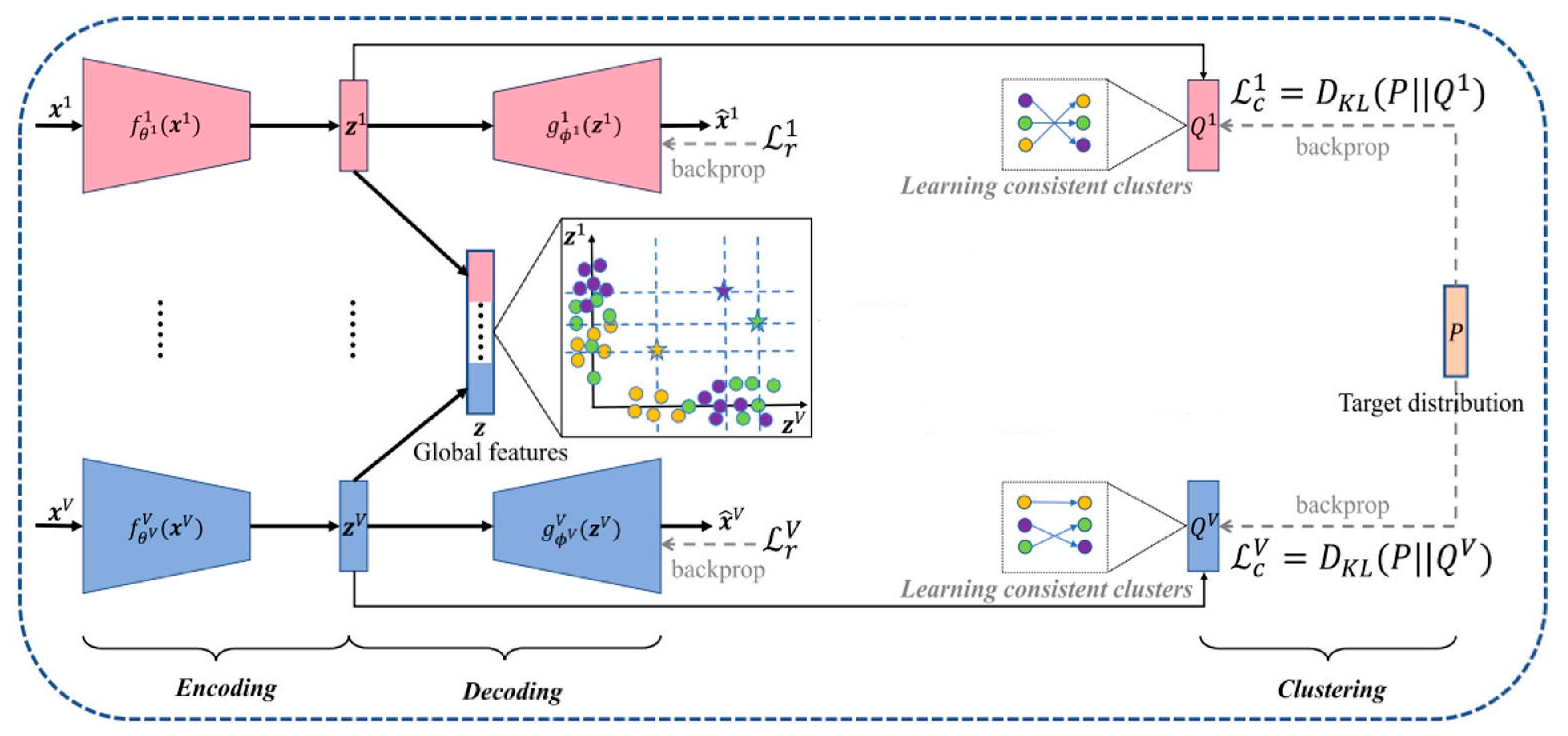
Kullback–Leibler (KL) divergence is a commonly used measure to quantify the difference between two probability distributions [23]. It is particularly useful in clustering tasks to evaluate how much the predicted cluster assignments deviate from the true distribution. The formula for KL divergence between two distributions $P$ and $Q$ is:

$$D_{KL}\left(P\parallel Q\right)=\sum _{i}P\left(i\right)\log \left(P\left(i\right)/Q\left(i\right)\right)$$

(12)

where $P$ represents the true distribution and $Q$ represents the predicted distribution. KL divergence is always non-negative and equals zero only when $P=Q$ for all $i$. In clustering, minimizing KL divergence helps align the predicted and true distributions, thus improving clustering accuracy.

In our approach, KL divergence is utilized to optimize the fusion of multi-view data. The model first performs view fusion to obtain a shared feature representation, denoted $Z$, which integrates the information from all views. This shared feature is then passed through an autoencoder framework, where KL divergence is used to minimize the difference between the predicted cluster distribution and the target distribution. The target probability distribution $P$, which serves as the “ground truth” distribution for training, is typically used in clustering tasks and functions similarly to soft labels. By minimizing KL divergence, we ensure that the learned representation $Z$ aligns closely with the true cluster structure, thereby improving the clustering performance.

3.2. Model Overview

DMVC-LSTM is an optimized framework specifically designed for multi-view data clustering problems. It aims to integrate information from different views, extract shared feature representations, and improve clustering performance through LSTM networks. The overall architecture of this model consists of the following key modules.

• Multi-View Feature Extraction

Each view’s data are processed independently using multi-layer neural networks to extract view-specific feature representations. The feature extractor structure for each view is identical, ensuring the comparability of the extracted features.

2.

Feature Fusion and Shared Representation

Feature fusion can be accomplished through three common mechanisms: concatenation, averaging, and attention-based methods. In this paper, we adopt concatenation for feature fusion. Firstly, concatenation is a simple and efficient method that merges features from multiple views. Secondly, concatenation enables the model to capture the consistency between different views, which helps the LSTM network better utilize its memory units to process and learn from the fused features. This approach ensures that each view’s unique contribution is preserved, facilitating the learning of more accurate and comprehensive representations.

3.

LSTM Autoencoder

The fused shared feature representation is fed into an LSTM autoencoder. The autoencoder leverages LSTM’s powerful sequential modeling capabilities to capture complex inter-feature relationships. Simultaneously, it optimizes the reconstruction loss, ensuring that the extracted features are more suitable for clustering tasks.

4.

Dynamic Clustering Optimization

The features output by the LSTM are passed to the clustering module. By dynamically adjusting the target distribution, the clustering results are iteratively optimized. During the clustering process, the model dynamically updates the cluster centers and sample assignments based on the data characteristics.

This model employs an end-to-end training framework that tightly integrates feature extraction, feature fusion, feature optimization, and clustering steps, thereby significantly enhancing clustering performance. The overall architecture is clear, with tightly coordinated modules ensuring seamless interaction. The overall architecture of the DMVC-LSTM model is shown in Figure 1.

3.3. Model Details

The architecture of the DMVC-LSTM model consists of two main components: the LSTM-based clustering model and the pretraining autoencoder. Below is a concise description of each part.

• LSTM-Based Clustering Model

The LSTM-based clustering model processes multi-view data and learns complex feature relationships across views. Its structure is as follows.

• Input Layer: Takes in multi-dimensional feature data, where each data point is represented as a sequence of feature vectors, preserving sequential dependencies.
• LSTM Hidden Layer: The LSTM layer captures temporal dependencies between features. It outputs a condensed feature representation used for clustering. The number of units in the LSTM layer is chosen based on the complexity of the data.
• Output Layer: A fully connected layer using softmax activation assigns data points to one of the n clusters. The model is trained with KL divergence as the loss function, minimizing the difference between the predicted cluster probabilities and the target distribution.
• Optimization: The model is optimized using the Adam optimizer to adapt the learning rate during training, and accuracy is tracked to monitor performance.

2.

Pretraining with Autoencoder

The pretraining phase uses an autoencoder to learn useful feature representations before fine-tuning for clustering. Its components are as follows.

• Input Layer: The same multi-dimensional data as in the clustering model are input to the autoencoder.
• LSTM Layer: Similarly to the clustering model, the autoencoder uses an LSTM layer. In this case, the LSTM outputs a sequence of feature representations, preserving temporal dependencies.
• Time-Distributed Reconstruction Layer: The LSTM output is passed through a time-distributed fully connected layer, which reconstructs the original input data at each time step.
• Loss Function: During pretraining, the model uses mean squared error (MSE) to minimize the reconstruction error.
• Training and Weight Transfer: After pretraining, the LSTM layer weights from the autoencoder are transferred to the clustering model, enabling it to start with well-learned features for better clustering.

3.

Fine-Tuning for Clustering

After pretraining, the model is fine-tuned using clustering data. The fine-tuning process minimizes KL divergence to optimize cluster assignments, with target distributions updated periodically. Training continues until convergence, ensuring the model assigns data points to the correct clusters.

3.4. Objective Function

In multi-view clustering, the optimization objective of LSTM is to maximize clustering accuracy while minimizing redundancy between views. Let the dataset for each view be:

$$X_v=x_1^v,x_2^v,\dots ,x_n^v$$

(13)

where $x_i^v\in R^{d_v}$ represents the $i$-th data point in the $v$-th view and $d_v$ is the feature dimension of the view. LSTM dynamically adjusts and optimizes these feature representations through its internal memory cells. For each view $v$, LSTM processes the input sequence step by step, outputting optimized the feature representation $h_t^v$.

These output features are used as inputs for the clustering algorithm to improve the final clustering results. The overall optimization goal is to minimize the weighted clustering loss function across all views. The loss function considers the importance of each view and fuses information from different views using weighted fusion. The objective function for the optimization process can be expressed as:

$$L_{\mathrm{total}}=\sum _{v=1}^V{w}_v\cdot L_v\left(h_v,C\right)$$

(14)

where $L_v\left(h_v,C\right)$ is the loss computed based on the LSTM output features $h_v$ and the cluster center $C$. The loss is typically measured using the Euclidean distance between data points and cluster centers:

$$L_v\left(h_v,C\right)=\sum _{i=1}^n{\left|h_i^v-C_{y_i}\right|}^2$$

(15)

Here, $h_i^v$ represents the $i$-th data point’s features extracted by LSTM for the $v$-th view, $y_i$ denotes the cluster label of the $i$-th data point, and $C_{y_i}$ is the cluster center of cluster $y_i$.

3.5. Optimization

To improve the model’s generalization ability, LSTM training typically incorporates regularization terms to prevent overfitting. L2 regularization is often used to constrain the magnitude of weights, ensuring that the model does not rely excessively on input data. The L2-regularized objective function is as follows:

$$L_{\mathrm{total}\_\mathrm{reg}}=L_{\mathrm{total}}+\mathsf{\lambda }\sum _{v=1}^V{\left|W_v\right|}_2^2$$

(16)

Here, $\mathsf{\lambda }$ is the regularization coefficient and $W_v$ is the weight matrix of the LSTM network for the $v$-th view. This approach enables the LSTM-based multi-view clustering method to automatically adjust the contribution of each view, thereby enhancing clustering accuracy.

Efficient optimization algorithms, such as Adam and RMSprop, are required during the optimization process. These adaptive algorithms dynamically adjust the learning rate based on the momentum and variance of gradients, accelerating convergence and preventing gradient explosion or vanishing problems. The update equations for the Adam optimization algorithm are as follows:

$$m_t={\mathsf{\beta }}_1{m}_{t-1}+\left(1-{\mathsf{\beta }}_1\right)g_t$$

(17)

$$v_t={\mathsf{\beta }}_2{v}_{t-1}+\left(1-{\mathsf{\beta }}_2\right)g_t^2$$

(18)

$$\widehat{m_t}={\displaystyle \frac{m_t}{1-{\mathsf{\beta }}_1^t}}$$

(19)

$$\widehat{v_t}={\displaystyle \frac{v_t}{1-{\mathsf{\beta }}_2^t}}$$

(20)

$${\mathsf{\theta }}_{t+1}={\mathsf{\theta }}_t-\mathsf{\eta }{\displaystyle \frac{\widehat{m_t}}{\sqrt{\widehat{v_t}}+\mathsf{ϵ}}}$$

(21)

Here, $m_t$ and $v_t$ are the estimates of the momentum and the variance of the gradients, respectively. $g_t$ is the current gradient, $\mathsf{\eta }$ is the learning rate, and $\mathsf{ϵ}$ is a small value to prevent division by zero. The parameters ${\mathsf{\beta }}_1$ and ${\mathsf{\beta }}_2$ are the exponential decay rates for the moment estimates, typically set to values close to 1 (e.g., 0.9 and 0.999, respectively). $t$ represents the iteration number, which indicates the current step in the optimization process. By incorporating $t$ in the calculations of $m_t$ and $v_t$, the algorithm compensates for their bias toward zero during the initial iterations. ${\mathsf{\theta }}_t$ is the parameter vector (or weights) of the model at the $t$-th iteration. The update rule for ${\mathsf{\theta }}_t$ adjusts the model’s parameters based on the corrected estimates of momentum and variance of the gradients, helping to efficiently approach the optimal solution and improve convergence.

As training progresses, gradually reducing the learning rate allows LSTM to fine-tune its parameters, avoiding local optima in the later stages of training. The learning rate decay formula is as follows:

$${\mathsf{\eta }}_t={\displaystyle \frac{{\mathsf{\eta }}_0}{1+\mathsf{\alpha }t}}$$

(22)

Here, ${\mathsf{\eta }}_0$ is the initial learning rate, $\mathsf{\alpha }$ is the decay factor, and $t$ is the training step.

For clarity, the optimization process is summarized in Algorithm 1.

Algorithm 1: The Optimization of DMVC-LSTM

Input: Shared feature representation $Z$, hidden layer dimension $h$. Step 1: Initialize the regularization coefficient $\lambda$ and the weight matrix $W_v$ for the $v$-th view. Step 2: Optimize the reconstruction loss $L_{\mathrm{reconstruction}}=\mathrm{MSE}\left(Z,\widehat{Z}\right)$ via Equations (17)–(21). Step 3: Update the learning rate via Equation (22). Step 4: Initialize the cluster centers $C$, calculate the probability distribution $P$ of samples to centers, and dynamically optimize the target distribution $Q$ and clustering parameters until the model converges. Output: Clustering result $Y=\{y_1,y_2,\dots ,y_n\}$.

3.6. Computational Complexity Analysis

The computational complexity of the DMVC-LSTM model arises from several key components, including feature extraction, feature fusion, LSTM autoencoding, clustering, and optimization algorithms. Each of these steps has its own complexity, which together determines the model’s overall complexity.

• Feature Extraction: The feature extraction network involves two hidden layers with ReLU activation and a softmax classification layer. The complexity of the ReLU activation function is $O\left(d\right)$, where $d$ is the feature dimension, and the complexity of the softmax layer is $O\left(C\right)$, where $C$ is the number of categories. With $n$ samples, the total complexity is $O\left(nd+nC\right)$.
• Feature Fusion: For multi-view feature fusion, the complexity is determined by the fusion method. If concatenation or averaging is used, the complexity is $O\left(n{\sum }_{v=1}^V{d}_v\right)$, where $d_v$ represents the feature dimension of each view. The same complexity applies when using an attention mechanism, as it weights and sums features from multiple views.
• LSTM Forward and Backward Propagation: For each time step, the complexity of LSTM is $O\left(d_v^2\right)$, where $d_v$ is the feature dimension of the view. For sequence data of length $T$, the forward and backward propagation complexity for a single view is $O\left(T{d}_v^2\right)$. With $V$ views, the total complexity becomes $O\left(V\cdot T\cdot d_v^2\right)$.
• Clustering: Initializing each cluster has a complexity of $O\left(kd\right)$, where k is the number of clusters and d is the feature dimension. Calculating distances between samples and cluster centers has a complexity of $O\left(knd\right)$, and updating cluster centers also requires $O\left(knd\right)$.
• Optimizing: The Adam algorithm has a complexity of $O\left(V\cdot d_v^2\right)$ for each update, as it updates the weight matrix for each view. Regularization also has a complexity of $O\left(V\cdot d_v^2\right)$, as it involves traversing all view-specific weight matrices. The clustering loss function involves computing Euclidean distances, which requires $O\left(nd\right)$ complexity.

The total computational complexity of the DMVC-LSTM model is:

$$O\left(n\sum _{v=1}^V{d}_v+V\cdot T\cdot d^2+knd+V\cdot d_v^2\right)$$

(23)

This complexity depends on factors such as the data scale, number of views, number of clusters, and feature dimensions in the LSTM.

4. Experiments

The experiments were conducted on a system running Windows 11, with TensorFlow 2.18 as the deep learning framework, Python 3.10, and an Nvidia GeForce RTX 4090 GPU for accelerated computation. The development environment used was PyCharm 2024.3.

The following sections presents the experimental details.

4.1. Datasets

The experiments were conducted using six real-world datasets to evaluate the performance of different clustering algorithms. Detailed descriptions of these datasets are provided below:

• 100 Leaves [24] includes 1600 leaf images from 100 leaf categories, with 16 images per category. It provides three views, each with a feature dimension of 64, corresponding to texture, shape, and edge features of the leaves.
• BBC [25] consists of 4659 news articles from the BBC News corpus, covering multiple news topics. It provides four views, each with a feature dimension of 685, extracted using different text feature extraction methods, including bag of words and TF-IDF.
• 20 Newsgroups [26] contains 2000 articles from 20 newsgroups and exhibits high-dimensional sparse characteristics. It provides three views, each with a feature dimension of 500, based on term frequency features, TF-IDF features, and topic modeling features.
• HW2sources [27] consists of 2000 handwritten letter samples and provides two views. The first view has a feature dimension of 784, extracted based on pixel information. The second view has a feature dimension of 256, capturing the structural edge information of handwriting.
• movies617 [28] comprises 617 movies with features describing movie plots, actors, and metadata. It has two views: the first view has a feature dimension of 1878 based on textual features extracted from plot descriptions, and the second view has a feature dimension of 1398 based on structured metadata features.
• Wikipedia Articles [29] contains 693 Wikipedia articles covering multiple thematic domains. It provides two views: the first view has a feature dimension of 128, extracted using the bag-of-words model, and the second view has a feature dimension of 10, generated using topic modeling.

Table 2. Basic Information of Datasets.

Dataset	$\mathit{n}$	$\mathit{V}$	${\mathit{d}}_{\mathit{v}}$
100 Leaves	1600	3	64
BBC	4659	4	685
20 Newsgroups	2000	3	500
HW2sources	2000	2	784, 256
movies617	617	2	1878, 1398
Wikipedia Articles	693	2	128, 10

summarizes the basic information of the datasets, including the total number of samples, the number of views, and the feature dimensions of each view.

4.2. Algorithms for Comparison

To evaluate the performance of DMVC-LSTM, six representative algorithms were selected for comparison, as follows.

SC_best [6]: Performs spectral clustering on each view independently and selects the best clustering result from a single view as the final result. This method is commonly used as a baseline algorithm for multi-view clustering.

MVGL [30]: A graph-based multi-view clustering algorithm. It constructs graph structures corresponding to each view and uses graph learning to jointly model multi-view information, enhancing the characterization of data structures.

SwMC [2]: A multi-view clustering algorithm with self-weighted multi-graph learning. It uses an adaptive weighting mechanism to dynamically assign weights based on the contribution of each view, achieving efficient multi-view data fusion and reducing the influence of noisy views.

SwMPC [31]: A non-parametric weighted multi-view projection clustering algorithm based on structured graph learning. It combines structural graph learning with a non-parametric weighting mechanism and improves feature representation through projection learning, leading to better clustering performance.

MSC_IAS [32]: A multi-view subspace projection clustering algorithm based on completeness-aware similarity. It addresses the incompleteness issue in multi-view data by using completeness-aware similarity to achieve joint subspace representation across views.

GFSC [33]: A global spectral clustering algorithm based on self-expressive multi-view fusion. It learns inter-view relationships using a self-expressive model and achieves multi-view clustering through global graph fusion, making it suitable for jointly modeling linearly correlated views.

4.3. Evaluation Metrics

In multi-view clustering tasks, it is common to use evaluation metrics such as accuracy (ACC), normalized mutual information (NMI), adjusted Rand index (ARI), F score, precision, recall, and purity. Among these, it is popular to select three to five metrics for evaluation. In this work, we have chosen ACC, NMI, ARI, and purity as our evaluation metrics. Below is a brief description of each selected metric.

• Accuracy (ACC) measures the proportion of correctly clustered samples compared to the total number of samples. It provides a straightforward assessment of how well the clustering algorithm performs in assigning samples to the correct clusters.
• Normalized Mutual Information (NMI) measures the amount of shared information between the predicted cluster assignments and the true labels, normalized to account for differences in dataset size. A higher NMI indicates better clustering performance, with values ranging from 0 (no mutual information) to 1 (perfect alignment).
• Adjusted Rand Index (ARI) compares the similarity between the predicted cluster assignments and the true labels, adjusting for the possibility of random clustering. Its value ranges from −1 (completely dissimilar) to 1 (perfectly identical), with 0 indicating random clustering assignments.
• Purity (PUR) evaluates how well each cluster corresponds to a single true class by calculating the fraction of correctly assigned samples in each cluster. Higher purity indicates better clustering results where each cluster predominantly contains samples from a single class.

These metrics are widely used in multi-view clustering research and provide a comprehensive evaluation of clustering performance from different perspectives.

4.4. Main Parameter Settings

In this experiment, several key hyperparameters were set for training our model. The main settings are as follows.

• LSTM Hidden Layer Dimension: The number of hidden units in the LSTM layer is set to 256, enabling the model to capture complex temporal relationships and inter-feature dependencies in multi-view data.
• Maximum Iterations: The maximum number of iterations is set to 5000, providing sufficient time for the model to converge.
• Tolerance: The convergence tolerance is set to 0.001, meaning training stops when the change in the target distribution is smaller than this threshold.

These parameter settings were chosen based on preliminary experiments and literature guidelines to ensure efficient training and high-quality clustering performance.

4.5. Comparative Results Analysis

Table 3. Algorithm comparative results (mean value in %). The best-performing metrics are highlighted in bold.

Dataset	Method	ACC	NMI	ARI	PUR
	SC_best	51.91	33.04	51.76	87.82
	MVGL	44.90	42.72	84.56	66.68
	SwMC	63.23	92.29	71.50	98.19
100 Leaves	SwMPC	61.66	76.79	48.51	69.99
	MSC_IAS	73.87	90.16	84.85	69.80
	GFSC	50.91	77.75	52.54	90.35
	Ours	74.07	92.53	84.35	98.39
	SC_best	70.40	90.41	67.56	80.42
	MVGL	63.02	86.18	77.94	78.87
	SwMC	65.28	90.20	78.90	90.54
BBC	SwMPC	61.48	88.43	60.29	96.73
	MSC_IAS	75.31	87.51	80.37	91.20
	GFSC	70.52	87.23	69.13	87.23
	Ours	76.33	90.54	94.42	95.99
	SC_best	57.37	69.69	56.51	73.62
	MVGL	42.82	42.16	64.72	67.55
	SwMC	62.15	84.66	73.46	92.71
20 Newsgroups	SwMPC	64.75	70.09	57.71	76.28
	MSC_IAS	59.00	94.22	72.61	77.96
	GFSC	75.16	96.00	67.14	68.55
	Ours	75.38	96.29	84.49	92.96
	SC_best	64.73	97.82	53.54	59.00
	MVGL	58.02	57.70	52.01	60.34
	SwMC	69.60	98.69	80.46	92.74
HW2sources	SwMPC	49.95	84.40	48.07	77.59
	MSC_IAS	63.07	79.73	67.53	81.18
	GFSC	58.04	85.23	56.46	92.82
	Ours	69.86	98.94	80.68	93.11
	SC_best	66.22	97.03	73.76	75.24
	MVGL	66.29	63.41	60.57	79.75
	SwMC	46.97	98.10	65.97	84.55
movies617	SwMPC	49.97	84.11	68.48	87.25
	MSC_IAS	76.60	89.26	69.57	96.04
	GFSC	74.22	95.83	71.14	67.51
	Ours	76.83	97.86	73.97	96.34
	SC_best	61.91	88.58	73.55	84.99
	MVGL	51.59	60.72	59.83	75.43
	SwMC	54.84	66.94	67.12	79.25
Wikipedia Articles	SwMPC	60.75	74.15	77.74	87.91
	MSC_IAS	77.72	81.45	76.01	92.56
	GFSC	71.45	96.47	72.43	64.89
	Ours	79.14	98.53	80.79	95.54

presents the comparative results of DMVC-LSTM and the six other algorithms across six datasets. The evaluation metrics comprise ACC, NMI, ARI, and PUR. Due to the generally small variation in standard deviations, which does not significantly reflect clustering performance, we report only the mean values for convenience. For deep learning-based methods, we present the results on the test set to avoid overfitting.

From an overall perspective, DMVC-LSTM demonstrates outstanding clustering performance across all datasets, showcasing significant advantages in multi-view data feature extraction, view fusion, and dynamic optimization. It exhibits excellent stability and generalization capability. Below is a detailed analysis.

4.5.1. Overall Performance of Different Algorithms

Single-View Algorithm (SC_best)

SC_best performs poorly on most datasets, especially those with more views or higher feature dimensions (e.g., 20 Newsgroups, movies617). It is limited by its inability to leverage complementary information across views. For example, on the 100 Leaves dataset, SC_best achieves only 51.91% ACC, significantly lower than DMVC-LSTM’s 74.07%.

Graph-Based Multi-View Algorithms (MVGL, GFSC)

MVGL and GFSC use graph structures for multi-view integration, but struggle with noisy or high-dimensional data. MVGL, for instance, achieves only 42.82% ACC on the 20 Newsgroups dataset, far below DMVC-LSTM’s 75.38%. While GFSC performs better on certain datasets, it still lags behind DMVC-LSTM in complex scenarios like Wikipedia Articles.

Weighted Multi-View Algorithms (SwMC, SwMPC)

SwMC and SwMPC outperform single-view algorithms, achieving competitive results on many datasets. For example, SwMC reaches 90.20% NMI on the BBC dataset, near DMVC-LSTM’s 90.54%. However, SwMPC struggles with heterogeneous data, achieving only 48.51% ARI on 100 Leaves, much lower than DMVC-LSTM’s 84.35%.

Subspace Projection Algorithm (MSC_IAS)

MSC_IAS performs well on datasets like movies617 and Wikipedia Articles, but its overall performance is lower compared to DMVC-LSTM. For example, on Wikipedia Articles, MSC_IAS achieves 77.72% ACC, while DMVC-LSTM achieves 79.14%. Its performance suffers on complex datasets like 20 Newsgroups due to difficulties in handling high-dimensional features.

Our Method (DMVC-LSTM)

DMVC-LSTM achieves the best or near-best clustering performance across all datasets, fully demonstrating its superiority in multi-view clustering tasks. For instance, on the 20 Nnewsgroups dataset, DMVC-LSTM achieves 75.38% ACC and 96.29% NMI, significantly outperforming GFSC and SwMPC. The key advantage of DMVC-LSTM is its LSTM-based framework, which effectively models the complex interdependencies between views and optimizes clustering structures.

4.5.2. Cross-Dataset Performance Trends

From Table 3, it is evident that the performance of different algorithms varies significantly across datasets, reflecting the influence of data distribution and characteristics on clustering algorithm suitability.

• On low-dimensional datasets with minimal redundancy, such as 100 Leaves and BBC, DMVC-LSTM quickly uncovers clustering structures with ACC scores of 74.07% and 76.33%. Other methods like SwMC and MSC_IAS show competitive performance, but struggle with complex feature relationships.
• On high-dimensional and heterogeneous datasets like 20 Newsgroups and movies617, DMVC-LSTM consistently achieves high NMI and ARI scores, demonstrating its robustness to complex relationships. In contrast, SwMPC and MVGL struggle on these datasets.
• On datasets with intricate inter-view interactions, such as Wikipedia Articles, DMVC-LSTM achieves an ACC of 79.14%, outperforming all other methods.

4.5.3. Performance Summary

DMVC-LSTM consistently delivers superior clustering performance across all datasets, primarily due to LSTM’s ability to efficiently capture complex feature dependencies and its use of an efficient Adam optimization algorithm. Compared to traditional single-view methods and other multi-view approaches, DMVC-LSTM excels at handling diverse data structures, providing robust performance and strong generalization capabilities in multi-view clustering tasks.

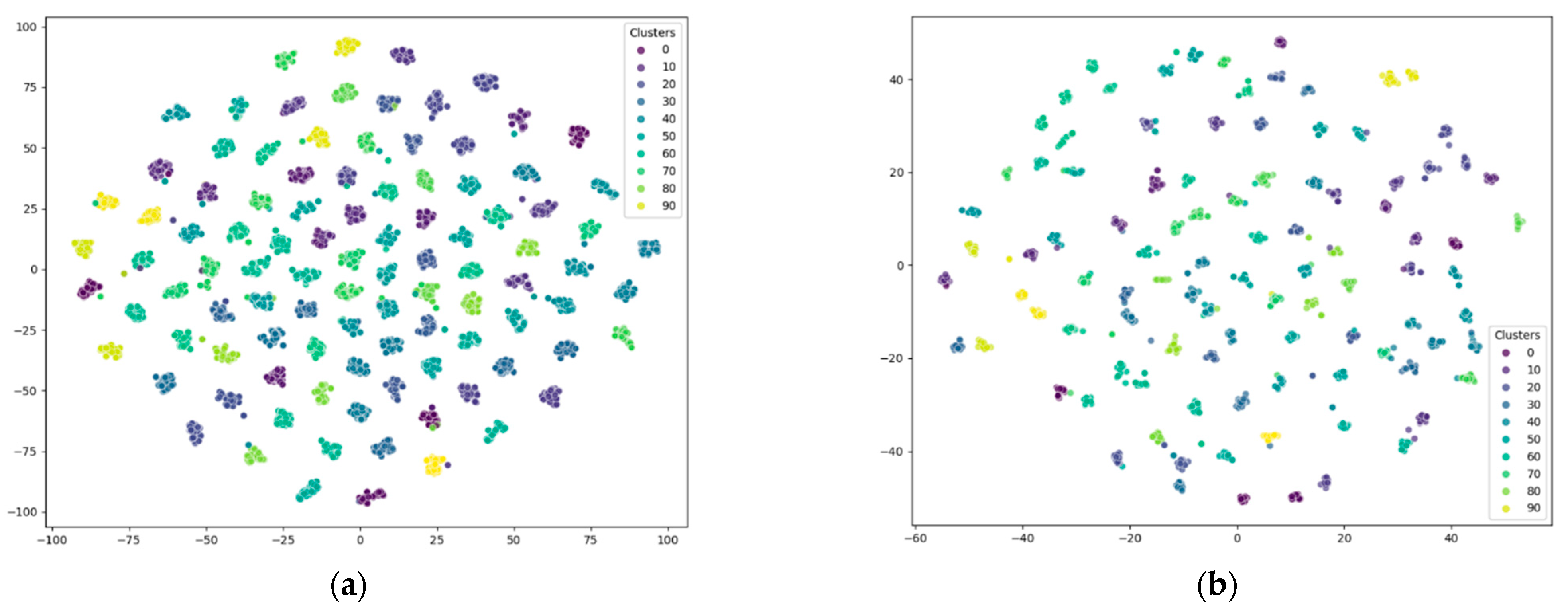
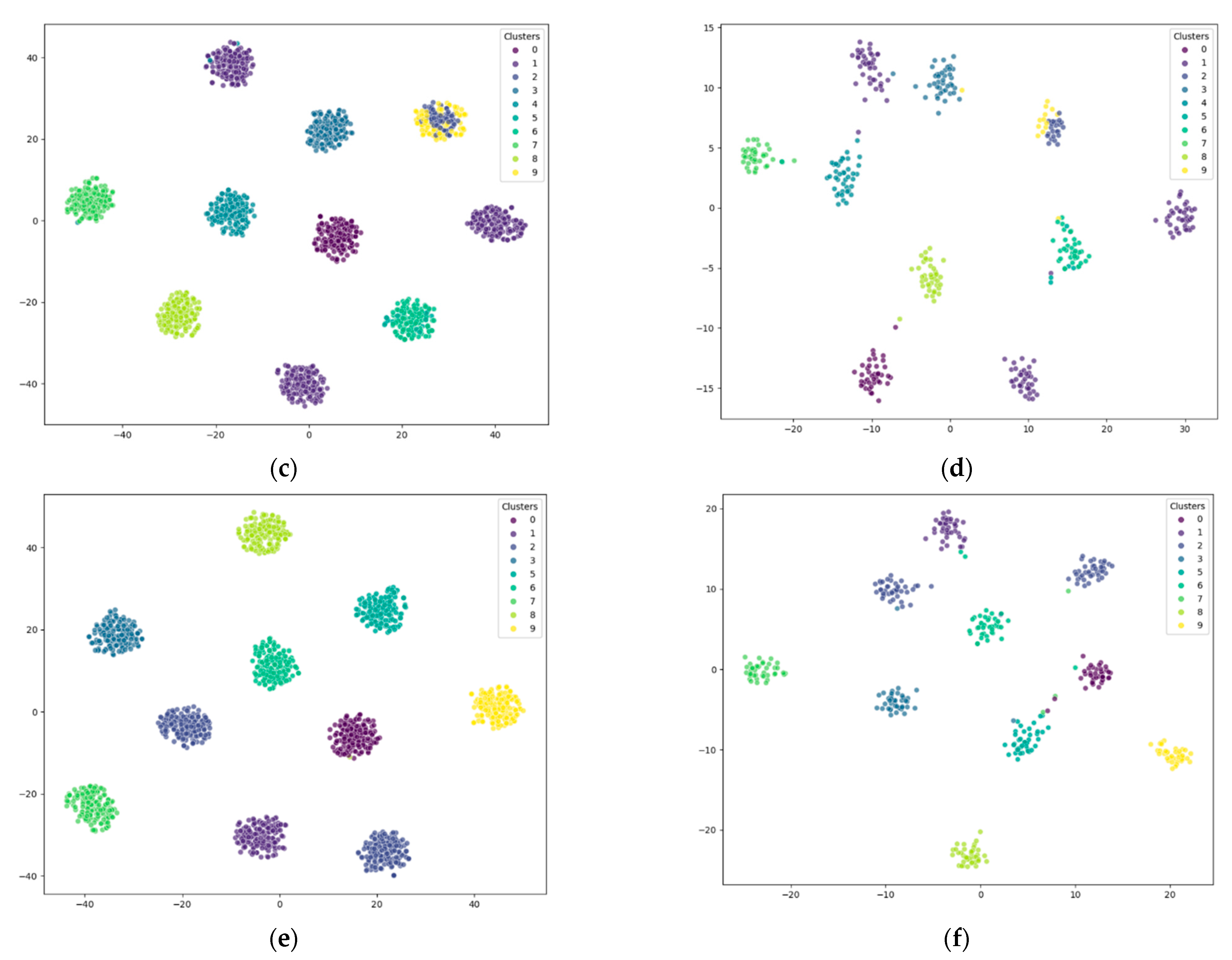
4.6. Visualization of Clustering

We conducted clustering experiments on six datasets: 100_Leaves, BBC, 20_Newsgroups, HW2sources, movies617, and Wikipedia_Articles, with the number of clusters set to 10. Figure 2 presents the clustering results for these datasets, where each cluster is distinguished by a unique color. Overall, our proposed DMVC-LSTM method successfully differentiates between various clusters, producing clear cluster boundaries.

In most cases, the clustering results demonstrate distinct separation between clusters, which indicates the robustness and effectiveness of our method. However, on the 20_Newsgroups dataset, there is some confusion between clusters 2 and 9, as their boundaries slightly overlap. Despite this, the clustering boundaries on the remaining datasets are well-defined, further validating the capability of DMVC-LSTM in handling high-dimensional and complex datasets.

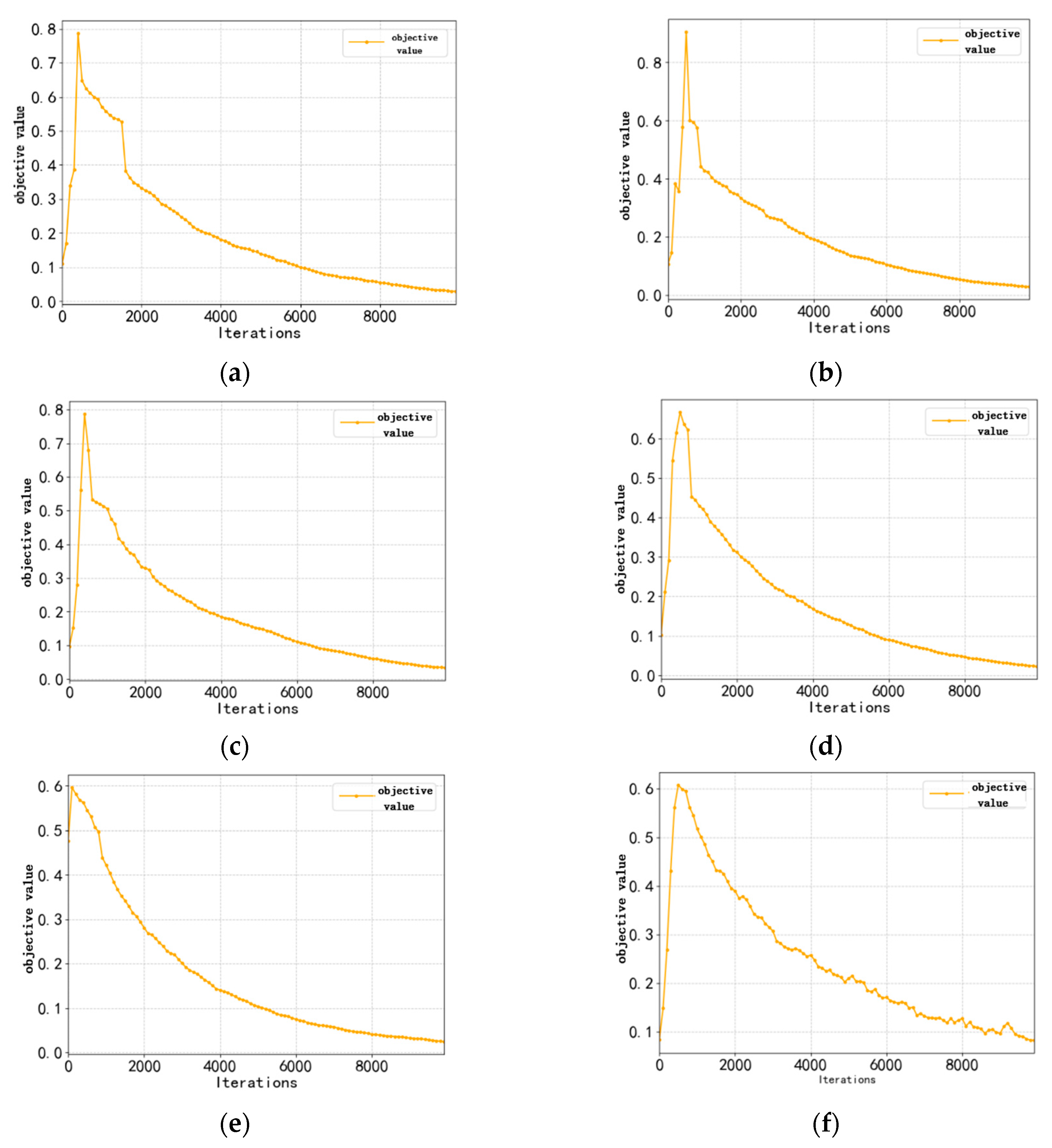
4.7. Convergence Analysis

To demonstrate the convergence of DMVC-LSTM, Figure 3 shows the changes in the objective function values over iterations across six datasets. As observed, the objective function values increase rapidly during the initial phase, followed by a gradual decline and eventual stabilization.

In all datasets, the rapid increase in objective function values during the early optimization stage is primarily attributed to the initial adjustments in weight allocation and feature modeling across multi-view data. As training progresses, the objective function values steadily decline and approach the optimal solution, demonstrating the model’s capability to dynamically adjust view weights and optimize clustering structures while effectively reducing redundancy. On most datasets, such as 20 Newsgroups and BBC, the decline process is smooth and efficient, reflecting DMVC-LSTM’s strong adaptability to the distributions of multi-view data.

Although slight fluctuations are observed in the convergence curve on the 100 Leaves dataset, likely due to higher redundancy among views, the overall trend remains stable. In contrast, the convergence curves on datasets like movies617 and Wikipedia Articles are smoother, indicating DMVC-LSTM’s robust performance in handling high-dimensional and complex data.

Overall, DMVC-LSTM demonstrates excellent convergence in optimizing the objective function. Minor fluctuations on specific datasets do not affect the model’s overall performance, as its dynamic fusion mechanism and deep feature modeling capabilities enable efficient optimization of multi-view data relationships, ultimately yielding stable and high-quality clustering results.

4.8. Parameter Sensitivity Analysis

To investigate the impact of hidden layer dimensions on the performance of the DMVC-LSTM model, we conducted experiments on the 100 Leaves dataset with hidden layer dimensions set to 32, 64, 128, 256, and 512. The results, including ACC and NMI metrics, are summarized in

Table 4. Impact of hidden layer dimensions on model performance (mean value in %).

Hidden Layer Dimension	ACC	NMI
32	62.13	86.42
64	68.07	89.27
128	72.49	91.04
256	74.07	92.53
512	71.43	90.98

.

As shown in Table 4, the hidden layer dimension significantly impacts the model’s clustering performance. When the dimension is small (e.g., 32 or 64), the performance is relatively poor, with ACC and NMI scores of 62.13% and 86.42% (dimension = 32) and 68.07% and 89.27% (dimension = 64). This indicates that smaller dimensions limit the model’s ability to capture complex interactions across views.

Increasing the hidden layer dimension leads to improved performance, peaking at 256 with an ACC of 74.07% and NMI of 92.53%. This demonstrates that a larger hidden layer enhances the model’s capacity to capture cross-view relationships and refine clustering boundaries. However, at 512, performance slightly declines (ACC = 71.43%, NMI = 90.98%), likely due to overfitting and feature redundancy.

Overfitting occurs when a large dimension makes the model prone to memorizing training data, reducing its generalization ability. Higher dimensions can also introduce redundant features that weaken the model’s overall performance.

These results highlight the importance of selecting an appropriate hidden layer dimension for DMVC-LSTM. For the 100 Leaves dataset, the optimal performance is achieved with a hidden layer dimension of 256, balancing accuracy and stability. Repeated experiments show minimal fluctuations in ACC and NMI (within ±0.5% and ±0.3%, respectively) at this dimension, suggesting enhanced robustness.

In summary, the hidden layer dimension is crucial for DMVC-LSTM’s performance. A dimension of 256 strikes the right balance between representational capacity and complexity, achieving optimal performance. Future work will explore automated parameter tuning, such as grid search or gradient-based optimization, to further streamline model configuration.

5. Conclusions

This paper introduces DMVC-LSTM, a novel approach that utilizes long short-term memory (LSTM) networks for multi-view clustering. While LSTM networks have been widely used in sequential data analysis, their potential in multi-view clustering has remained underexplored. DMVC-LSTM leverages LSTM’s ability to capture complex interdependencies and nonlinear relationships between different views, thereby enhancing clustering accuracy and robustness. The method employs three feature fusion strategies—concatenation, averaging, and attention-based fusion—with concatenation being the primary method due to its effectiveness in preserving view consistency. Additionally, DMVC-LSTM is especially effective for datasets with symmetrical relationships between views, maintaining underlying structures.

Experiments show that DMVC-LSTM outperforms existing algorithms, especially on high-dimensional and complex datasets, such as 20 Newsgroups and Wikipedia Articles. This work represents the first application of LSTM in multi-view clustering, marking a significant advancement in both clustering performance and the use of LSTM in multi-view data analysis.

Extending the DMVC-LSTM method to structural health monitoring and time-series data mining is a promising direction. In structural health monitoring, the challenges include handling data from multiple sensors, which may have varying levels of noise and temporal dependencies. DMVC-LSTM’s ability to model complex relationships between different sensor data views could provide a robust solution for these challenges. Similarly, in time-series data mining, where long-term dependencies and nonlinear relationships between time steps are critical, the proposed method could significantly improve prediction accuracy and robustness by capturing intricate temporal dependencies across views. By addressing these domain-specific challenges, DMVC-LSTM could lead to valuable advancements in real-world applications, offering a clearer roadmap for future research in these areas.

References

1. Chao, G.; Sun, S.; Bi, J. A survey on multi-view clustering. arXiv 2017, arXiv:1712.06246. [Google Scholar]
2. Nie, F.; Li, J.; Li, X. Self-weighted multiview clustering with multiple graphs. In Proceedings of the Twenty-Sixth International Joint Conference on Artificial Intelligence (IJCAI-17), Melbourne, Australia, 19–25 August 2017; pp. 2564–2570. [Google Scholar]
3. Xu, Y.M.; Wang, C.D.; Lai, J.H. Weighted multi-view clustering with feature selection. Pattern Recognit. 2016, 53, 25–35. [Google Scholar] [CrossRef]
4. Xu, C.; Tao, D.; Xu, C. A survey on multi-view learning. arXiv 2013, arXiv:1304.5634. [Google Scholar]
5. Likas, A.; Vlassis, N.; Verbeek, J.J. The global k-means clustering algorithm. Pattern Recognit. 2003, 36, 451–461. [Google Scholar] [CrossRef]
6. Ng, A.; Jordan, M.; Weiss, Y. On spectral clustering: Analysis and an algorithm. Adv. Neural Inf. Process. Syst. 2001, 14. [Google Scholar]
7. Bickel, S.; Scheffer, T. Multi-view clustering. In Proceedings of the Fourth IEEE International Conference on Data Mining (ICDM’04), Brighton, UK, 1–4 November 2004; Volume 4, pp. 19–26. [Google Scholar]
8. Fu, L.; Lin, P.; Vasilakos, A.V.; Wang, S. An overview of recent multi-view clustering. Neurocomputing 2020, 402, 148–161. [Google Scholar] [CrossRef]
9. Yang, Y.; Wang, H. Multi-view clustering: A survey. Big Data Min. Anal. 2018, 1, 83–107. [Google Scholar] [CrossRef]
10. Gönen, M.; Margolin, A.A. Localized data fusion for kernel k-means clustering with application to cancer biology. Adv. Neural Inf. Process. Syst. 2014, 27. [Google Scholar]
11. Du, L.; Zhou, P.; Shi, L.; Fan, M. Robust multiple kernel k-means using l21-norm. In Proceedings of the Twenty-Fourth International Joint Conference on Artificial Intelligence, Buenos Aires, Argentina, 25–31 July 2015. [Google Scholar]
12. Zheng, Q.; Zhu, J.; Ma, Y.; Li, Z.; Tian, Z. Multi-view subspace clustering networks with local and global graph information. Neurocomputing 2021, 449, 15–23. [Google Scholar] [CrossRef]
13. Du, G.; Zhou, L.; Yang, Y.; Lü, K.; Wang, L. Deep multiple auto-encoder-based multi-view clustering. Data Sci. Eng. 2021, 6, 323–338. [Google Scholar] [CrossRef]
14. Xu, J.; Ren, Y.; Tang, H.; Pu, X.; Zhu, X.; Zeng, M.; He, L. Multi-VAE: Learning disentangled view-common and view-peculiar visual representations for multi-view clustering. In Proceedings of the IEEE/CVF International Conference on Computer Vision, Montreal, QC, Canada, 10–17 October 2021; pp. 9234–9243. [Google Scholar]
15. Hochreiter, S. Long Short-term Memory. Neural Comput. 1997, 9, 1735–1780. [Google Scholar] [CrossRef] [PubMed]
16. Lange, S.; Riedmiller, M. Deep auto-encoder neural networks in reinforcement learning. In Proceedings of the 2010 International Joint Conference on Neural Networks (IJCNN), Barcelona, Spain, 18–23 July 2010; IEEE: Piscataway, NJ, USA, 2010; pp. 1–8. [Google Scholar]
17. Huang, P.; Huang, Y.; Wang, W.; Wang, L. Deep embedding network for clustering. In Proceedings of the 2014 22nd International Conference on Pattern Recognition, Stockholm, Sweden, 24–28 August 2014; IEEE: Piscataway, NJ, USA, 2014; pp. 1532–1537. [Google Scholar]
18. Opochinsky, Y.; Chazan, S.E.; Gannot, S.; Goldberger, J. K-autoencoders deep clustering. In Proceedings of the ICASSP 2020-2020 IEEE International Conference on Acoustics, Speech and Signal Processing (ICASSP), Barcelona, Spain, 4–8 May 2020; IEEE: Piscataway, NJ, USA, 2020; pp. 4037–4041. [Google Scholar]
19. Dong, S.; Xu, H.; Zhu, X.; Guo, X.; Liu, X.; Wang, X. Multi-view deep clustering based on autoencoder. J. Phys. Conf. Ser. 2020, 1684, 012059. [Google Scholar] [CrossRef]
20. Ghasedi Dizaji, K.; Herandi, A.; Deng, C.; Cai, W.; Huang, H. Deep clustering via joint convolutional autoencoder embedding and relative entropy minimization. In Proceedings of the IEEE International Conference on Computer Vision, Venice, Italy, 22–29 October 2017; pp. 5736–5745. [Google Scholar]
21. Lim, K.L.; Jiang, X.; Yi, C. Deep clustering with variational autoencoder. IEEE Signal Process. Lett. 2020, 27, 231–235. [Google Scholar] [CrossRef]
22. Medsker, L.R.; Jain, L. Recurrent neural networks. Des. Appl. 2001, 5, 2. [Google Scholar]
23. Kullback, S.; Leibler, R.A. On information and sufficiency. Ann. Math. Stat. 1951, 22, 79–86. [Google Scholar] [CrossRef]
24. Beghin, T.; Cope, J.S.; Remagnino, P.; Barman, S. Shape and texture based plant leaf classification. In Advanced Concepts for Intelligent Vision Systems, Proceedings of the 12th International Conference, ACIVS 2010, Sydney, Australia, 13–16 December 2010; Proceedings, Part II 12; Springer: Berlin/Heidelberg, Germany, 2010; pp. 345–353. [Google Scholar]
25. Greene, D.; Cunningham, P. Practical solutions to the problem of diagonal dominance in kernel document clustering. In Proceedings of the 23rd International Conference on Machine Learning, Pittsburgh, PA, USA, 25–29 June 2006; pp. 377–384. [Google Scholar]
26. Lang, K. Newsweeder: Learning to filter netnews. In Proceedings of the Machine Learning Proceedings 1995, Tahoe City, CA, CA, 9–12 July 1995; Morgan Kaufmann: Burlington, MA, USA, 1995; pp. 331–339. [Google Scholar]
27. Wang, H.; Yang, Y.; Liu, B.; Fujita, H. A study of graph-based system for multi-view clustering. Knowl. Based Syst. 2019, 163, 1009–1019. [Google Scholar] [CrossRef]
28. Available online: https://lig-membres.imag.fr/grimal/data.html (accessed on 4 December 2024).
29. Available online: http://www.svcl.ucsd.edu/projects/crossmodal/ (accessed on 4 December 2024).
30. Zhan, K.; Zhang, C.; Guan, J.; Wang, J. Graph learning for multiview clustering. IEEE Trans. Cybern. 2017, 48, 2887–2895. [Google Scholar] [CrossRef]
31. Wang, R.; Nie, F.; Wang, Z.; Hu, H.; Li, X. Parameter-free weighted multi-view projected clustering with structured graph learning. IEEE Trans. Knowl. Data Eng. 2019, 32, 2014–2025. [Google Scholar] [CrossRef]
32. Wang, X.; Lei, Z.; Guo, X.; Zhang, C.; Shi, H.; Li, S.Z. Multi-view subspace clustering with intactness-aware similarity. Pattern Recognit. 2019, 88, 50–63. [Google Scholar] [CrossRef]
33. Kang, Z.; Shi, G.; Huang, S.; Chen, W.; Pu, X.; Zhou, J.T.; Xu, Z. Multi-graph fusion for multi-view spectral clustering. Knowl. -Based Syst. 2020, 189, 105102. [Google Scholar] [CrossRef]
Figure 1. The overall architecture of DMVC-LSTM.
Symmetry 17 00161 g001
Figure 2. Clustering results on different datasets. (a) 100_Leaves. (b) BBC. (c) 20_Newsgroups. (d) HW2sources. (e) movies617. (f) Wikipedia_Articles.
Symmetry 17 00161 g002aSymmetry 17 00161 g002b
Figure 3. Convergence curves of DMVC-LSTM. (a) movies617. (b) Wikipedia Articles. (c) 20 Newsgroups. (d) BBC. (e) HW2sources. (f) 100 Leaves.
Symmetry 17 00161 g003