Article

ASGT-Net: A Multi-Modal Semantic Segmentation Network with Symmetric Feature Fusion and Adaptive Sparse Gating

1
School of Information and Control Engineering, Qingdao University of Technology, Qingdao 266520, China
2
State Key Laboratory of Ecological Safety and Sustainable Development in Arid Lands, Xinjiang Institute of Ecology and Geography, Chinese Academy of Sciences, Urumqi 830011, China
3
Xinjiang Key Laboratory of Biodiversity Conservation and Application in Arid Lands, Xinjiang Institute of Ecology and Geography, Chinese Academy of Sciences, Urumqi 830011, China
*
Author to whom correspondence should be addressed.
Symmetry 2025, 17(12), 2070; https://doi.org/10.3390/sym17122070
Submission received: 27 October 2025 / Revised: 28 November 2025 / Accepted: 1 December 2025 / Published: 3 December 2025
(This article belongs to the Section Computer)

Abstract

In the field of remote sensing, accurate semantic segmentation is crucial for applications such as environmental monitoring and urban planning. Effective fusion of multi-modal data is a key factor in improving land cover classification accuracy. To address the limitations of existing methods, such as inadequate feature fusion, noise interference, and insufficient modeling of long-range dependencies, this paper proposes ASGT-Net, an enhanced multi-modal fusion network. The network adopts an encoder-decoder architecture, with the encoder featuring a symmetric dual-branch structure based on a ResNet50 backbone and a hierarchical feature extraction framework. At each layer, Adaptive Weighted Fusion (AWF) modules are introduced to dynamically adjust the feature contributions from different modalities. Additionally, this paper innovatively introduces an alternating mechanism of Learnable Sparse Attention (LSA) and Adaptive Gating Fusion (AGF): LSA selectively activates salient features to capture critical spatial contextual information, while AGF adaptively gates multi-modal data flows to suppress common conflicting noise. These mechanisms work synergistically to significantly enhance feature integration, improve multi-scale representation, and reduce computational redundancy. Experiments on the ISPRS benchmark datasets (Vaihingen and Potsdam) demonstrate that ASGT-Net outperforms current mainstream multi-modal fusion techniques in both accuracy and efficiency.

1. Introduction

Remote sensing technology, as a key means of obtaining information about the Earth’s surface, has important applications in urban planning, disaster monitoring, agricultural management, ecological protection and other fields [1,2]. With technological advances, the resolution of remote sensing images is constantly improving, which can present the shape, texture and spatial distribution of features in more detail. The intricate nature of remote sensing images imposes greater demands on image processing methods. Especially in semantic segmentation tasks, the accurate identification and categorization of features have come into sharp focus [3,4,5].
For semantic segmentation tasks involving remote sensing imagery, classical approaches frequently utilize features that are handcrafted, alongside low-level visual indicators, for the purpose of classification. However, this approach struggles to capture intricate details and semantic relationships, particularly in complex scenes with fine features and hyperspectral targets. Additionally, these methods typically require extensive prior knowledge, involve cumbersome preprocessing steps, and exhibit limited generalization abilities [6,7]. In comparison, advanced deep learning methodologies, particularly the convolutional neural network (CNN) architecture, exhibit exceptional proficiency in extracting robust features from remote sensing images for segmentation tasks, thereby leading to a substantial improvement in the precision of feature recognition [8,9,10]. The visual transformer (ViT), by effectively utilizing its self-attention mechanism, demonstrates remarkable proficiency in capturing global dependencies within data. Consequently, it offers significant advantages when applied to high-resolution imagery, where the ability to grasp long-range correlations is crucial [11,12].
Although the above deep learning methods have certain advantages in semantic segmentation of remote sensing images, most of them are used in a single modality, while the current semantic segmentation using multi-modal data is the inevitable trend, and multi-modal fusion can effectively improve the performance. The limitations of using single-modal data in managing intricate scenes are progressively emerging as the clarity of remote sensing imagery increases, thereby posing significant hurdles in obtaining satisfactory segmentation outcomes. As a result, the integration of multi-modal data has risen to prominence as a pivotal strategy for augmenting the precision of semantic segmentation in remote sensing imagery. By integrating diverse modal data sources, including RGB imagery and Digital Surface Models (DSM), one can harness the complementary information inherent between these modalities to bolster the feature representation prowess of the model. However, remote sensing multi-modal fusion extends beyond just RGB and DSM data and encompasses other types, such as LiDAR and hyperspectral data. LiDAR provides precise terrain and elevation information, while hyperspectral data offers rich spectral features that can significantly enhance target recognition and classification accuracy. Yet, the fusion of these data types presents multiple challenges, such as differences in scale, noise interference, and computational complexity, all of which require innovative fusion techniques to address effectively [13,14]. This, in turn, enhances the classification precision and enhances the robustness of the model against various perturbations [15,16].
However, while multi-modal data fusion offers significant benefits, it also presents numerous challenges [17,18]. Current multi-modal data fusion faces the following main problems: Firstly, most existing multi-modal data fusion methods, especially CNN and ViT based models, usually rely on basic fusion methods such as simple splicing or addition. Although these methods achieve basic feature fusion, they lack effective feature selection and weighting mechanisms, resulting in poor feature fusion between different modalities. A recent study by Zhang et al. proposed the S2DBFT model, which utilizes a dual-branch design to handle hyperspectral data by fusing spectral and spatial features [19]. This approach highlights the importance of capturing the interaction between spectral and spatial features, a challenge that our hybrid CNN-Transformer architecture addresses through innovative fusion strategies. Secondly, as remote sensing image resolution increases, the computational demands of ViT models rise sharply. Processing high-resolution images significantly increases inference time and computational costs, posing substantial obstacles to practical applications. Finally, although ViT excels at capturing global features, it tends to overlook local details, particularly when addressing small-scale targets or complex scenes, leading to reduced segmentation accuracy. Therefore, achieving a balance between global feature modeling and the preservation of local details remains a critical issue that requires further exploration [20,21,22,23].
To address the aforementioned challenges, this paper introduces an enhanced multi-modal fusion network, ASGT-Net. This network effectively resolves issues such as insufficient feature fusion, high computational complexity, and the loss of local details found in existing methods. By utilizing a phased approach for feature extraction and fusion, ASGT-Net seamlessly integrates the extensive global modeling capabilities of ViT with the robust local feature extraction prowess of CNN, thereby enhancing its overall performance. It proficiently manages diverse multi-modal datasets, extracts exhaustive and multi-faceted features, and minimizes computational overhead, it is highly adaptable for the intricate process of segmenting high-resolution remote sensing imagery into meaningful semantic categories. Below is an overview of the key achievements of this research project:
(1)
This paper proposes an innovative multi-modal fusion network architecture that integrates ViT and CNN. In this fusion architecture, the ViT component incorporates a Learnable Sparse Attention (LSA) module, replacing the traditional self-attention mechanism, which significantly reduces computational complexity. This design allows ASGT-Net to effectively lower the computational burden while retaining the powerful feature extraction capabilities of Transformers.
(2)
During feature fusion, the CNN part employs an Adaptive Weighted Fusion (AWF) module, which dynamically adjusts feature weights based on different modalities to emphasize key information and enhance fusion effectiveness. Simultaneously, the ViT module integrates an Adaptive Gating Fusion (AGF) mechanism that alternates with the LSA module, optimizing inter-modal information exchange and facilitating effective integration of global and local features.
(3)
Through rigorous comparative experiments on the ISPRS Vaihingen and Potsdam datasets, results demonstrate that ASGT-Net significantly improves segmentation performance while maintaining low computational complexity, outperforming other state-of-the-art multi-modal fusion methods. These experiments validate ASGT-Net’s superiority in efficiently fusing multi-modal data, enhancing accuracy, and improving computational efficiency.
In light of the above discussion, we next provide an overview of the related work that underpins our framework.

2. Related Works

2.1. Semantic Segmentation of Remote Sensing Imagery

Semantic segmentation aims to assign a semantic label to each pixel in remote sensing images. High-resolution imagery is particularly challenging due to complex backgrounds, multi-scale objects, large intra-class variations and severe foreground–background imbalance, which limit the performance of early CNN-based methods. Fully convolutional networks (FCNs) introduced skip connections to fuse low- and high-level features and significantly improved segmentation accuracy. The DeepLab family [24] further strengthened multi-scale context modeling by combining dilated convolutions with spatial pyramid pooling. Encoder–decoder architectures such as U-Net [25], SegNet [26], and DeconvNet [27] are effective at recovering spatial resolution and object boundaries, and remain strong baselines for remote-sensing semantic segmentation.

2.2. Semantic Segmentation with CNN–Transformer Architectures

To overcome the locality of conventional CNNs, Transformer-based architectures have recently been introduced into remote-sensing segmentation. Originating from NLP, Transformers are powerful in modeling long-range dependencies through global self-attention, and ViT variants have achieved strong performance on image classification and semantic segmentation tasks [28,29,30]. However, naïve global attention is computationally expensive for large, high-resolution images [31,32,33,34,35,36].
To improve efficiency, many studies adopt sparse or localized attention [37]. Swin Transformer [35] restricts self-attention to shifted windows, reducing complexity while still capturing global context. Sparse Transformer [37], Longformer [38] and BigBird [39] propose different sparse attention patterns that combine local and global tokens, enabling scalable processing of long sequences and large images. In parallel, hybrid CNN–Transformer architectures exploit the complementary strengths of local convolution and global attention [40,41].For example, PVT [34] and DPT [42] integrate CNN backbones with Transformer blocks and have shown clear gains on remote-sensing segmentation benchmarks.

2.3. Multi-Source Data Fusion for Semantic Segmentation

Multi-modal fusion is an effective way to improve segmentation accuracy and robustness by combining complementary geospatial data such as RGB/VIS imagery, Digital Surface Models (DSM), Digital Elevation Models (DEM) and LiDAR point clouds [43,44,45,46,47,48]. Recent work by Wang et al. [49], for example, fuses multi-temporal optical images with DEM data and demonstrates clear benefits in complex terrain, which is consistent with our motivation for VIS–DSM fusion.
Early fusion strategies mainly rely on simple concatenation or fixed weighted summation, which often introduce redundancy and fail to fully exploit modality-specific information. To address this, feature-level attention modules such as SE and CBAM [50] are used to re-weight channel responses and improve fusion quality. More recently, cross-modal attention within Transformer frameworks has been adopted to dynamically integrate multi-modal features and enhance segmentation performance [51,52,53]. Hu et al. [54] proposed the TMFF framework for sewer defect classification, further highlighting the importance of flexible fusion mechanisms for complex multi-source data.
Despite these advances, many fusion approaches still suffer from either over-redundant representations or insufficient use of inter-modal complementarity. Gated fusion has therefore emerged as a more flexible solution [55,56,57,58]. By learning data-dependent gating weights, it adaptively controls the contribution of each modality and suppresses redundant information, leading to more discriminative fused features. Representative methods such as SA-GATE [59] show that gated fusion can effectively optimize information flow in complex scenes while keeping the computational cost manageable. This line of research directly motivates our design of an adaptive gated fusion module for VIS–DSM integration.

3. Math

In designing the ASGT-Net architecture, we draw inspiration from recent advances in multi-modal fusion and hybrid CNN–Transformer frameworks. YCANet [60] demonstrates that combining heterogeneous sensors (e.g., camera and LiDAR) can significantly enhance feature representation and robustness. This motivated our fusion of VIS and DSM modalities to leverage their complementary spatial and structural information.
In addition, the dual-branch design of ASGT-Net is inspired by DeepU-Net [61], which shows that parallel branches are effective for capturing multi-scale variations in high-resolution remote sensing imagery. These findings provide useful architectural precedents for our encoder design.
The overall ASGT-Net architecture is illustrated in Figure 1. It consists of three main components: (1) a CNN-based feature extraction and preliminary fusion module, (2) a Transformer-based deep processing and fusion module that alternates LSA and AGF blocks for local–global context modeling, and (3) a decoder that progressively restores spatial resolution. Shallow high-resolution features are combined with deep semantic features through skip connections to preserve fine-grained spatial details in the final segmentation.
ASGT-Net takes VIS images and DSM data as inputs. First, the feature representation and preliminary fusion module uses convolutional layers to map both modalities into a high-dimensional feature space and applies an adaptive weighted fusion mechanism, ensuring effective integration of complementary VIS–DSM information. The fused features are then passed to a Transformer-based deep processing and fusion module, where LSA and AGF blocks are alternately stacked to further enhance multi-modal feature interaction and global context modeling. In the decoding stage, a cascaded upsampling structure is adopted: early layers use bilinear interpolation to restore spatial resolution, while later layers employ transposed convolutions to refine structural details. Skip connections are used to combine shallow high-resolution features with deep semantic representations, enabling the final segmentation results to be both accurate and detail-preserving.

3.1. Feature Representation and Preliminary Fusion Coding Module

This module aims to extract basic features from different modalities and perform an initial fusion, providing a compact and informative representation for the subsequent encoder–decoder stages. By integrating complementary VIS and DSM information at an early stage, it enhances feature robustness while reducing redundancy.
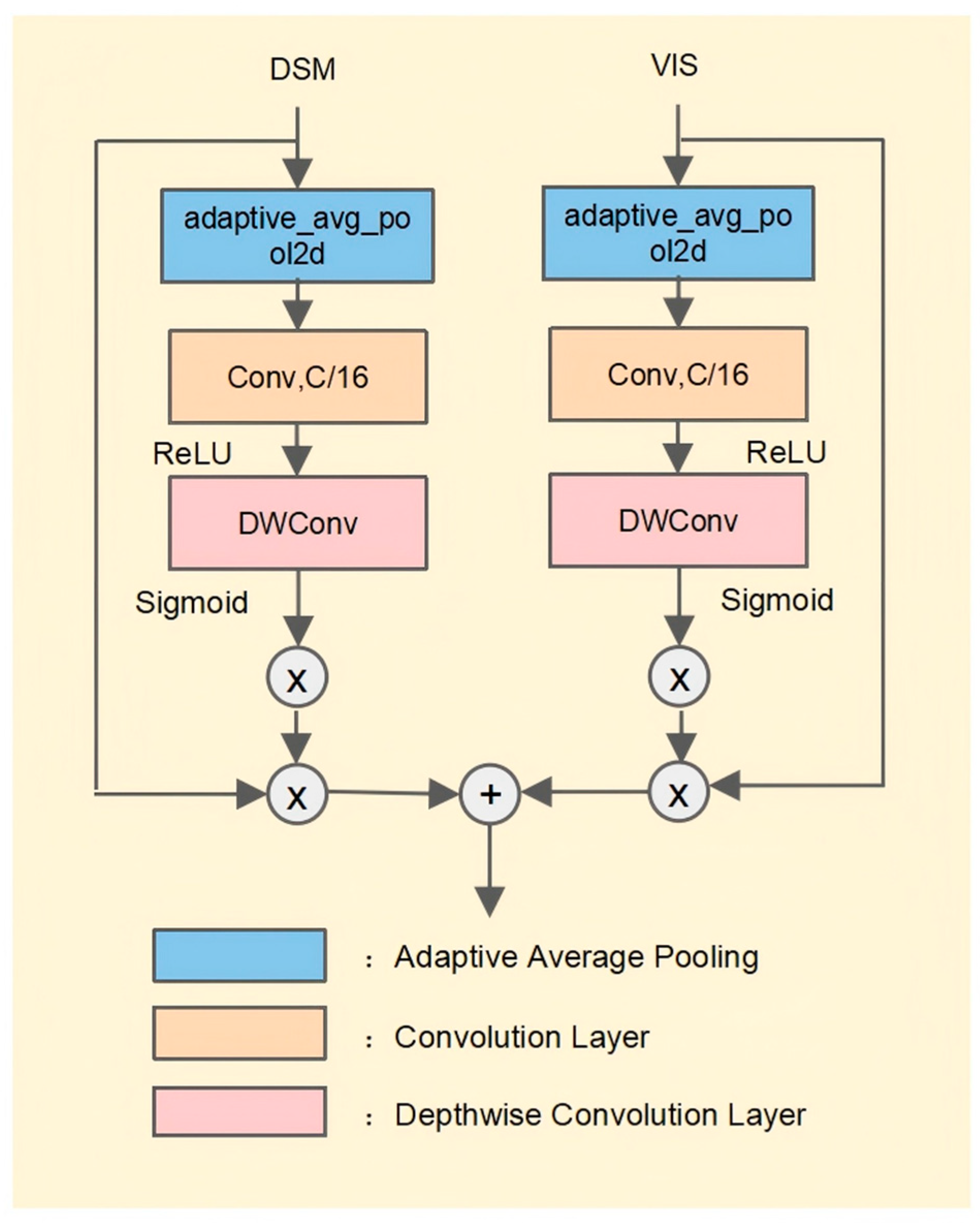
As shown in Figure 2, the AWF module adopts a dual-branch architecture built on an enhanced ResNet-50 backbone to process VIS images and DSM data in parallel. In each branch, features with C channels are first passed through global average pooling to capture global context. The pooled descriptor is then fed into a 1 × 1 convolution followed by a ReLU activation, and a depthwise 1 × 1 convolution is further applied to refine the representation with low computational cost. Finally, a sigmoid activation produces adaptive scalar weights ω y and ω x for the DSM and VIS features, respectively.
These weights are used to adaptively fuse the two modalities as:
o u t p u t = ω y · D S M _ f e a t u r e s + ω x · V I S _ f e a t u r e s .
Here, ω y and ω x are scalar weights per feature map, obtained from global context. The number of trainable parameters in each AWF layer depends on the input channel size; in our network, the four AWF layers have approximate parameter counts of 768, 9216, 34,816, and 135,168, respectively. This design allows the network to adaptively fuse multimodal features while keeping the computational cost manageable.

3.2. Deep Feature Processing and Fusion Coding Module

After feature representation and initial fusion, the deep processing and fusion module further integrates multi-modal features using a 12-layer Transformer-based encoder. VIS and DSM features are first mapped to a shared embedding space and then fed into this encoder, which interleaves LSA blocks with AGF blocks to achieve progressive enhancement and fusion.
Specifically, the encoder is composed of four stages, each containing three layers. LSA blocks focus on selectively activating the most informative spatial positions, while AGF blocks perform modality-aware fusion of VIS and DSM features. By alternating LSA and AGF (three LSA layers followed by three AGF layers, repeated twice), the encoder gradually refines global context and cross-modal interactions.
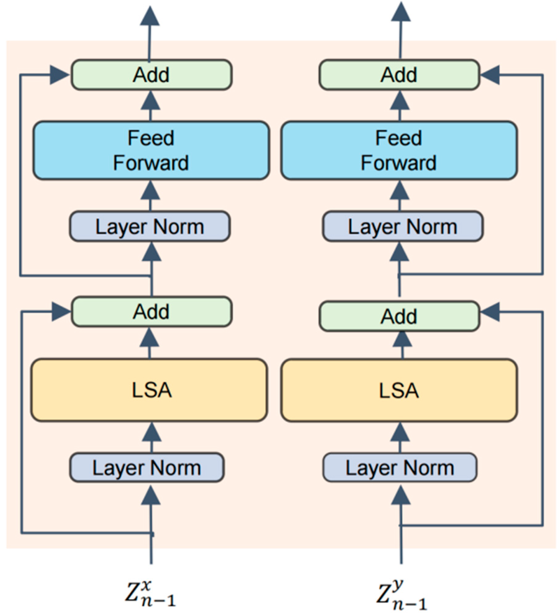
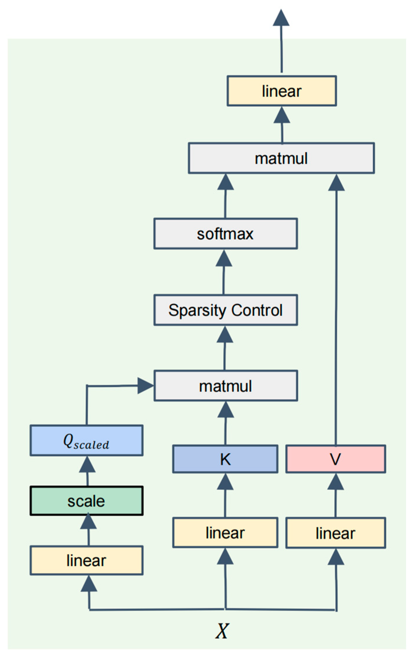
The LSA block extends the standard Transformer self-attention layer by introducing a learnable sparsity mechanism, which reduces redundant attention computations and improves efficiency. Its overall structure is illustrated in Figure 3, and the internal computation flow (Q/K/V projection, sparse attention, and output projection) is summarized in Figure 4.
Given the input feature sequence X , we first obtain the query ( Q ), key ( K ) and value ( V ) matrices through linear projections.
Q = X W q , K = X W k , V = X W v .
Following the standard multi-head self-attention formulation, the attention scores are computed as:
A = Q K T d k
where d k is the key dimension.
After computing the attention matrix, we introduce a sparsity control mechanism to improve computational efficiency and suppress uninformative responses. We use a learnable scalar s and map it to a sparsity ratio α ∈ (0,1) via a sigmoid function:
α = σ s , σ x = 1 1 + e x
The ratio α then controls the degree of sparsification in the subsequent Top-K operation.
We then apply the sparsity ratio α to the attention matrix by Top-K sparsification. For each batch b, head h and query position i, we keep only the top-k attention scores and discard the rest. Let N be the number of keys; the number of retained elements is:
k = α N
and the threshold τ b , h , i for each query position i is the k-th largest value among the attention scores of each key position:
τ b , h , i = T o p K _ t h { A b , h , i , 1 , , A b , h , i , N } , k
A binary mask M is then obtained by comparing each score with τ b , h , i :
M b , h , i , j = 1 ,   i f   A b , h , i , j τ b , h , i , 0 , otherwise .  
The sparsified attention matrix A s p is defined as:
A b , h , i , j s p = A b , h , i , j ,   i f   M b , h , i , j = 1 , , i f   M b , h , i , j = 0  
and is followed by a standard softmax. The sparsity parameter α is initialized to 0.5 and learned jointly with the network parameters, so that the model adaptively focuses on important attention entries while suppressing less relevant ones.
The specific implementation steps are shown in Algorithm 1.
Algorithm 1: LSA Module with Top-K Sparsification
Input: feature sequence X R B × N × C , number of attention heads H , learnable sparsity parameter s
Output: output features X R B × N × C
 1.
  Compute linear projections: Q , K , V Linear X
 2.
  Reshape Q , K , V to B , H , N , C / H
 3.
  Scale queries: Q Q / C / H
 5.
  Compute attention scores: A Q K
 5.
  Compute sparsity ratio: α σ s
 6.
  For each batch b , head h , and query i :
6.1
k α N
6.1
τ b , h , i TopK _ th A b , h , i , : , k
6.3
Generate mask
  • M b , h , i , j 1 if A b , h , i , j τ b , h , i else 0
 7.
  End for
 8.
  Sparsify attention:
  • A b , h , i , j sp A b , h , i , j if M b , h , i , j = 1 ,
  • A b , h , i , j sp if M b , h , i , j = 0
 9.
  Apply softmax: A sp softmax A sp
 10.
Apply dropout: A sp Dropout A sp
 11.
Weighted sum of values: X A sp V
 12.
Output projection and dropout: X Dropout Proj X
In our experiments, setting k = 20% yields a good trade-off between accuracy and efficiency; the learned α typically converges to values between 0.4 and 0.7 across layers, indicating effective sparsity control.
Given the sparsified attention matrix A s p , we apply a standard softmax along the key dimension and use the resulting weights to aggregate the value matrix V :
O = S o f t m a x A s p V .
The aggregated features are then projected by a linear layer to produce the final output of the LSA block:
X ^ = O W o u t .
where W o u t signifies the parameter matrix for the output linear transformation layer, whereas X ^ indicates the resultant feature vector that serves as the final output.
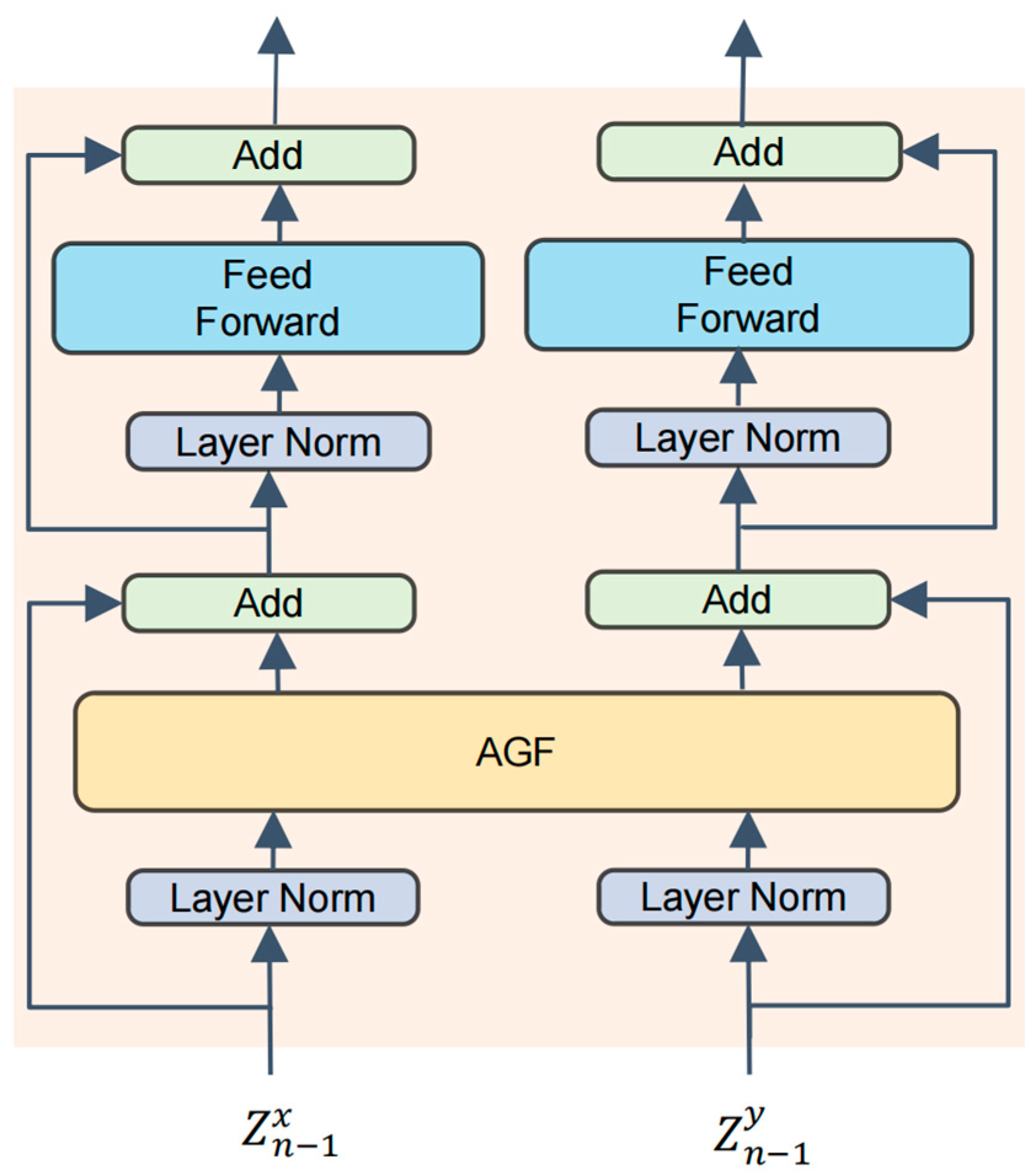
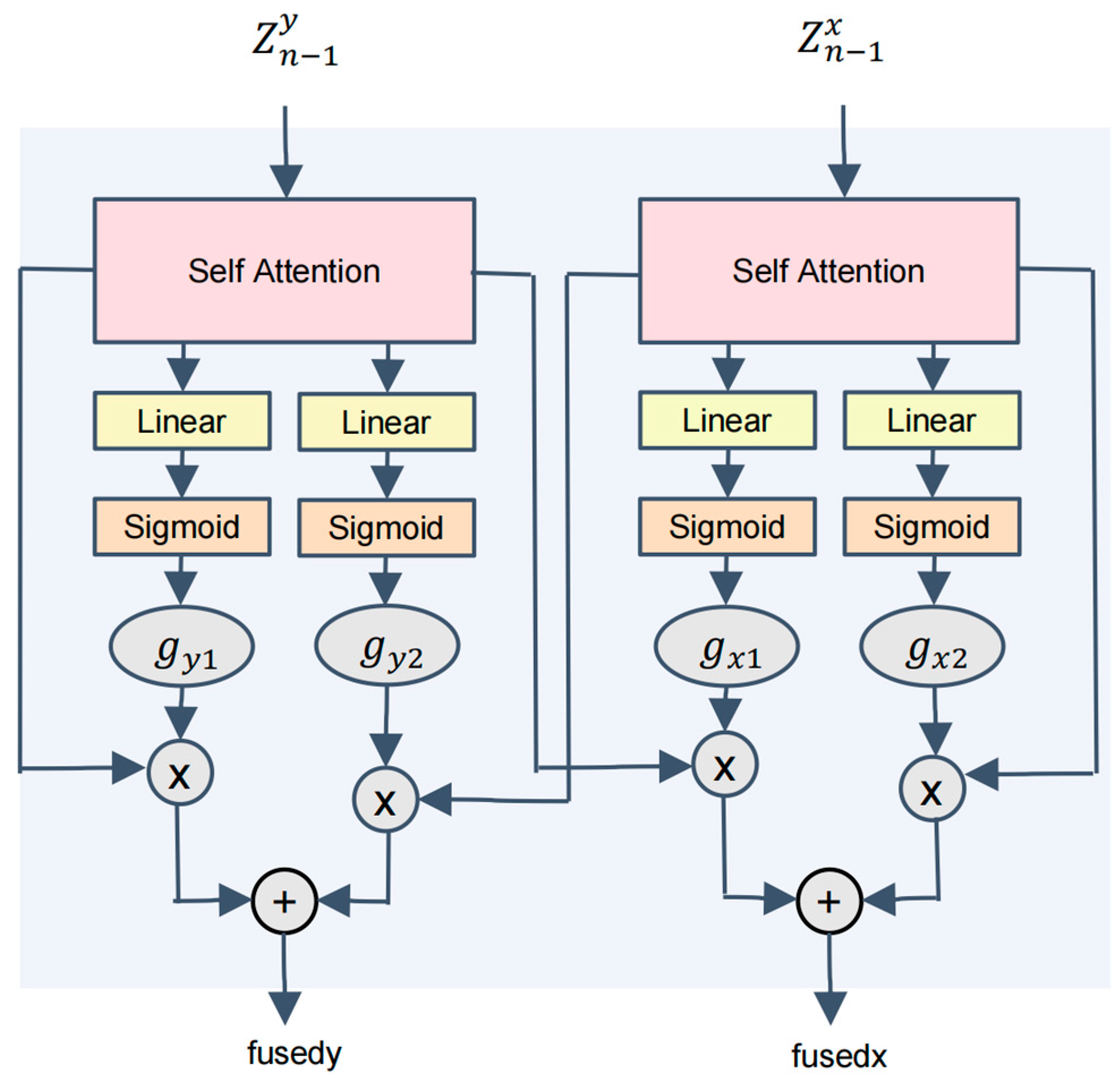
The AGF block shares a similar topology with the LSA block, but is designed for deep fusion of VIS and DSM features rather than sparse attention. Its overall structure is illustrated in Figure 5, and the internal computation flow is shown in Figure 6.
Given the input features Z n 1 x and Z n 1 y from the two modalities, we first apply self-attention independently to obtain enhanced representations:
a t t e n t i o n s x = s e l f a t t e n t i o n Z n 1 x
a t t e n t i o n s y = s e l f a t t e n t i o n Z n 1 y .
Next, four spatial gating maps g y 1 , g y 2 , g x 1 , g x 2 are generated by lightweight gating networks with a linear transformation followed by a sigmoid activation:
g x 1 = σ W x 1 a t t e n t i o n s x
g x 2 = σ W x 2 a t t e n t i o n s x
g y 1 = σ W y 1 a t t e n t i o n s y ,
g y 2 = σ W y 2 a t t e n t i o n s y
where W x 1 , W x 2 , W y 1 , W y 2 are learnable weight matrices and σ(·) denotes the sigmoid function. The gating maps g x 1 , g x 2 , g y 1 , g y 2 have the same shape [C, H, W] as the input features, enabling pixel-wise and channel-wise control of the fusion ratios in the range [0, 1].
Finally, the two modality features are fused in a bidirectional manner as:
f u s e d x = g x 1 a t t e n t i o n s x + g x 2 a t t e n t i o n s y ,
f u s e d y = g y 1 a t t e n t i o n s y + g y 2 a t t e n t i o n s x .
where ⊙ denotes element-wise multiplication. This design allows AGF to adaptively balance self-information and cross-modal information for each spatial location.

3.3. Decoding and Feature Reconstruction Module

Within the decoding and feature restoration component, the model first re-establishes the spatial configuration of the feature representation, and then rebuilds the features through a well-organized sequence of decoding units. Initially, decoding blocks use bilinear interpolation for up-sampling, while the final layer employs inverse convolution to achieve precise feature recovery. Each decoding module integrates feature information from the corresponding level of the encoder with the current feature map using skip connection technology, achieving efficient consolidation of multi-scale features. The resultant fused feature maps undergo a sequence of two 3 × 3 convolutional operations, Subsequently, the application of Batch Normalization and the ReLU activation function is employed to further enhance and refine the feature representation. Throughout this entire procedure, the initial convolutional layer serves to adjust the quantity of feature map channels in accordance with subsequent processing steps, whereas the subsequent layer primarily focuses on extracting intricate spatial and semantic nuances.
The Segmentation Head performs the ultimate refinement of the up-sampled and reconstructed feature maps, ultimately yielding high-resolution semantic segmentation outcomes. It transforms the final feature map into pixel-wise classification outputs, enabling the complete reconstruction of detailed and semantic information from the input image.

4. Experiments and Discussions

4.1. Datasets and Initial Preparation

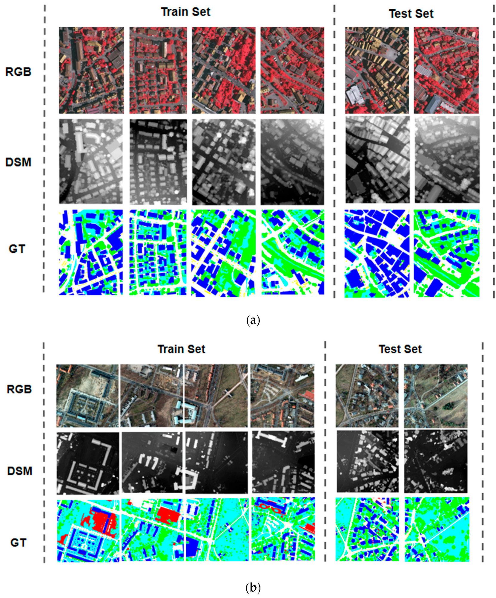
The datasets from Vaihingen and Potsdam were the basis for the experimental data in this study. Illustrative samples from these datasets, encompassing orthophotos, DSM images, and corresponding labeled maps, are depicted in Figure 7.
The Vaihingen dataset encompasses high-resolution remote sensing imagery captured in Vaihingen, Germany, featuring a pixel spacing of 0.09 m. It encompasses six distinct categories: impervious surfaces, structures, low vegetation, trees, vehicles, and a miscellaneous group. The dataset includes multispectral images as well as Digital Surface Model (DSM) data. In the experimental setup, a total of twelve image segments (specifically, with IDs: 1, 3, 23, 26, 7, 11, 13, 28, 17, 32, 34, and 37) were utilized for the training phase, whereas four image segments (specifically, with IDs: 5, 21, 15, and 30) were designated for the testing phase. Each of these segments was accompanied by corresponding ground truth labels for evaluation purposes.
The Potsdam dataset includes high-resolution RS imagery of Potsdam, Germany, with 0.05 m/px res, covering urban elements like buildings, roads, veg, trees, cars, & other features. It also provides multi-spectral imagery (NIR, R, G, B) & DSM data. 22 image segments are used for training (ID: 2_10, 2_11, 2_12, 3_10, 3_11, 3_12, 4_10, 4_11, 4_12, 5_10, 5_11, 5_12, 6_7, 6_8, 6_9, 6_10, 6_11, 6_12, 7_7, 7_8, 7_11, 7_12) and 14 image clips were used for testing (ID: 2_13, 2_14, 3_13, 3_14, 4_13, 4_14, 4_15, 5_13, 5_14, 5_15, 6_13, 6_14, 6_15, 7_13), and all image clips were accompanied by ground truth labels.
To ensure effective model training, we performed detailed preprocessing on the dataset. All image pixel values were normalized to the [0, 1] range to reduce illumination differences and accelerate model convergence. DSM values were normalized per image using min-max normalization, i.e., for each DSM image, the minimum value was subtracted and divided by the range (maximum–minimum). Large images were first preprocessed and resized to 1024 × 1024 pixels. These preprocessed images were then divided into 256 × 256 patches using a sliding window with a stride of 32 pixels. Each preprocessed image produces 25 patches along each dimension, resulting in a total of 625 patches per image. Ground truth labels were converted from RGB color coding to numerical labels, with boundary regions refined for accuracy. To enhance model generalization, data augmentation including random horizontal and vertical flips and arbitrary rotations was applied. Importantly, DSM patches were extracted using the same sliding window coordinates as RGB patches, ensuring that each DSM patch is spatially aligned with its corresponding RGB patch.

4.2. Assessment of Indicators

To objectively evaluate segmentation performance, we utilize OA, mF1, and mIoU. Derived from the confusion matrix, these metrics measure overall correctness, average class-wise F1-Score, and average IoU.
O A = T P + T N T P + F N + F P + T N
P r e c i s i o n = T P T P + F P
R e c a l l = T P T P + F N
F 1 = 2 P r e c i s i o n × R e c a l l P r e c i s i o n + R e c a l l
I o U = T P T P + F P + F N
During the assessment of classification tasks, the terms TP, TN, FP, and FN are employed to signify correctly classified positives, negatives, misclassified positives, and misclassified negatives, respectively, serving as metrics for assessing the accuracy of classifying positive and negative instances. Based on these metrics, the overall average F1 score and IoU for all classes, termed as mF1 and mIoU, were computed.

4.3. Implementation Details

In this experiment, we use the PyTorch 2.1.0 deep learning framework and perform all training on an NVIDIA RTX 3090 GPU with 24 GB of memory under a CUDA 11.8 environment. In our setup, training with a batch size of 10 takes about 1.2 s per iteration, with a peak memory usage of approximately 14 GB, which demonstrates that the proposed LSA module significantly reduces the cost of full self-attention while maintaining accuracy.
The model is initialized from the pre-trained R50 + ViT-B_16 backbone to enhance feature extraction capability; each branch starts from its corresponding ImageNet-pretrained weights. The model is trained for 50 epochs with a batch size of 10. Early stopping is applied with a patience of 7 epochs and a minimum delta of 0.001 to prevent overfitting. All input data are standardized prior to feature extraction and fusion. To mitigate class imbalance in remote sensing datasets, we employ a weighted cross-entropy loss function and incorporate a dynamic sparsity control mechanism. The sparsity learning rate (sparsity_lr) is initialized to 0.001 and updated after each iteration using the same MultiStepLR schedule as the base learning rate, ensuring synchronized sparsity adjustment throughout training. An L1 regularization term with coefficient λ = 1 × 10⁻⁴ is added to strengthen sparsity constraints and improve model generalization. Gradient clipping is not applied.
For optimization, we use Stochastic Gradient Descent (SGD) with an initial learning rate of 0.01, momentum of 0.9, and weight decay of 0.0005. The MultiStepLR scheduler decays the learning rate at epochs 25, 35, and 45 with a decay factor γ = 0.1. To assess the influence of randomness and ensure reproducibility, each experiment is repeated three times with different random seeds (42, 3407, 2025) for PyTorch, NumPy, and Python’s random module. All reported performance metrics are computed as the average over these three runs to provide stable and reliable estimates.
A summary of the training hyperparameters is provided in Table 1.

4.4. Comparative Experiments

We conducted a detailed evaluation of our model on the Vaihingen and Potsdam datasets, comparing it with a range of advanced methods that encompass attention mechanisms, hybrid convolution–Transformer designs, and multi-scale feature fusion strategies. To ensure fair comparison, all baseline models were re-trained using the same input modalities (VIS + DSM) and consistent training settings, including batch size, optimizer, learning rate schedule, and data preprocessing. The evaluation focused on key performance metrics such as OA, mF1, and mIoU.
All baseline models were retrained under identical experimental settings to ensure fair comparison. Official implementations were used whenever available; for methods lacking complete official code, missing components (e.g., data preprocessing or training procedures) were faithfully re-implemented based on the original papers. Unless otherwise specified, the CNN and Transformer backbones of both our method and all baseline models are initialized with ImageNet-pretrained weights. The baselines included in our study are either originally designed to support multi-modal inputs or can be adapted to VIS + DSM by adding a lightweight DSM branch without modifying their backbone architectures. For methods that already provide DSM-specific branches or fusion modules, we strictly follow their official designs. For RGB-only architectures, VIS and DSM are treated as two separate input modalities and fed into modality-specific branches, and multi-modal feature fusion is carried out inside the network, while keeping the original backbone structures unchanged. These design choices ensure a fair and consistent comparison across all methods. In contrast, some recently proposed Transformer-based approaches are not included because adapting them to multi-modal inputs (VIS + DSM) would require substantial architectural changes, which could significantly affect the comparability and fairness of the experimental results.
Table 2 showcases the comparative results obtained on the Vaihingen dataset. The proposed method achieves an OA of 92.30%, surpassing the performance of all other benchmarked models. It demonstrates exceptional segmentation performance across various categories, including buildings, low vegetation, and cars, with an mF1 of 90.88% and a mIoU of 83.65%. Additionally, the model excels in multi-modal feature fusion and fine-grained segmentation tasks, with classification accuracy in several categories surpassing other methods. In the building segmentation task, the method achieves an accuracy of 97.76%, significantly outperforming other models, demonstrating its strong ability to handle building boundaries in complex scenes. For low vegetation segmentation, it also exhibits excellent classification performance, with an accuracy of 82.18%, surpassing other methods. This indicates that the model is able to effectively distinguish low vegetation from other similar categories (e.g., trees and clutter), especially in cases with complex backgrounds or similar textures. Notably, the method excels in small target segmentation tasks (e.g., cars), achieving an accuracy of 90.33%, far exceeding other methods. This result highlights the method’s advantage in handling very small-scale targets, particularly when the targets are extremely small or partially occluded, as it maintains high precision and robustness through multi-modal information fusion.
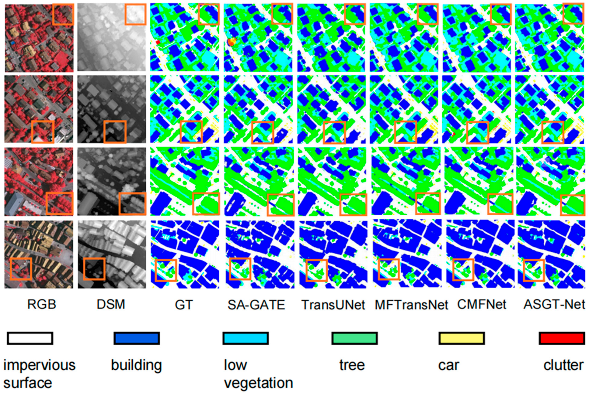
The visual representations of segmentation outcomes depicted in Figure 8 highlight notable discrepancies in the model performances for delineating building boundaries and identifying low vegetation categories within the Vaihingen dataset. In the first two rows of results, as unimodal models, SA-GATE and TransUNet perform relatively weakly when dealing with building boundaries, especially when the building is similar to the ground features or the edges are occluded. The segmentation results are often imprecise, with blurred boundaries and poor building integrity. In contrast, MFTransNet and CMFNet enhance boundary segmentation accuracy by incorporating DSM height information, allowing for clearer depiction of building outlines. However, ASGT-Net excels in these scenarios, not only producing more accurate boundaries but also preserving the overall shape of the building better, demonstrating excellent robustness in complex situations. In the third row, despite the similarity in color and texture between low vegetation and other categories (such as trees and clutter), ASGT-Net effectively integrates DSM height information to more efficiently distinguish low vegetation, surpassing other models in classification performance. Other methods tend to confuse low vegetation with trees, while the proposed approach enhances the ability to differentiate complex categories by efficiently fusing multi-modal information, particularly in detail processing and category distinction. In the fourth row, ASGT-Net performs exceptionally well in small target segmentation tasks (such as cars), effectively handling small targets that are occluded or similar to the background. By fusing multi-modal information, it accurately recognizes and segments targets, even in cases with low contrast or partial occlusion, outperforming other techniques. This demonstrates a significant advantage in small target segmentation, maintaining high precision and robustness in complex backgrounds and small-scale target scenarios.
The quantitative data derived from analyzing the Potsdam dataset is outlined in Table 3. Our model achieves a significant OA of 91.24%, showing particularly robust performance in the areas of buildings and trees. The model’s mF1 rating reaches 92.30% and the mIoU is as high as 86.10%, which shows the efficient segmentation capability in complex scenes. Compared with other methods, the model has obvious advantages in overall classification performance. On this dataset, the model also demonstrated excellent performance in building and tree segmentation, further validating its segmentation capability in detail processing and complex scenes.
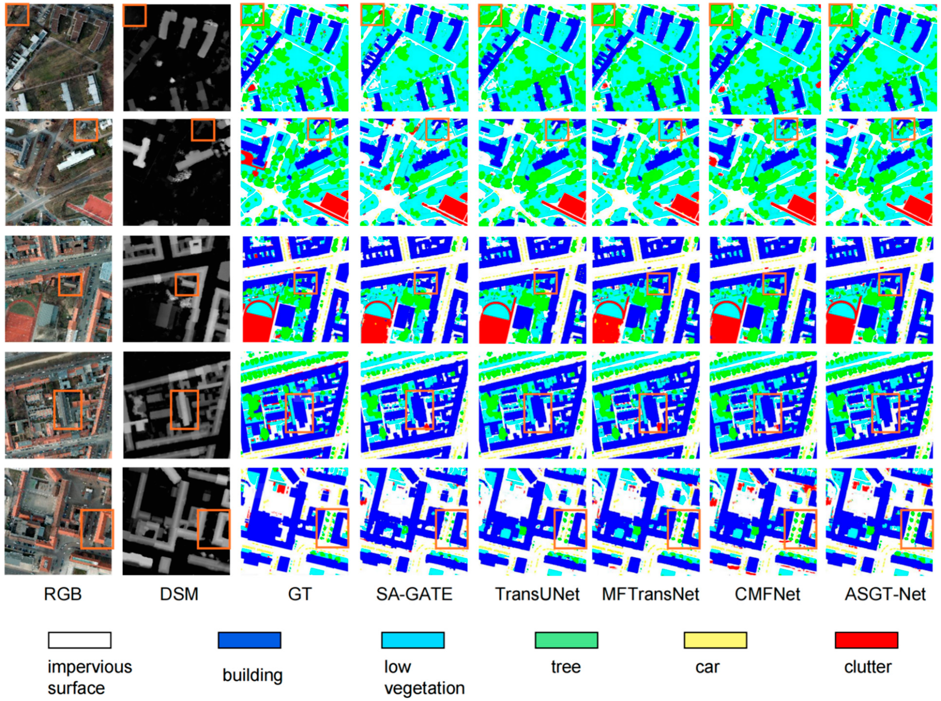
Figure 9 illustrates the visualization outcomes for the Potsdam dataset. Upon inspection, it is evident that the unimodal models, namely SA-GATE and TransUNet, exhibit slightly inferior performance in the segmentation tasks involving buildings and low vegetation., especially in the distinction between building and road boundaries with some ambiguity. The segmentation results of these models are not precise enough when dealing with complex scenes, particularly in cases of ambiguous building boundaries or occlusion. In contrast, MFTransNet and CMFNet significantly improve the processing of building boundaries by introducing DSM height information, leading to a noticeable improvement in the portrayal of building contours. In the first row, ASGT-Net excels in the segmentation task of low vegetation, effectively distinguishing it from other similar categories. The second, third, and fourth rows demonstrate its strong capability in building segmentation within complex scenes, particularly in handling building boundaries and intricate backgrounds, where it can clearly segment building contours, reduce noise, and enhance accuracy. The fifth row highlights the advantage of this approach in small target segmentation (e.g., cars), accurately identifying targets that are occluded or similar to the background, showcasing high precision and robustness.
Table 4 reports the per-seed results of ASGT-Net on the Vaihingen and Potsdam datasets, showing that performance fluctuations across different random seeds are minimal, confirming the stability and reproducibility of our method.

4.5. Ablation Experiment

The ablation study involved two experimental configurations, assessing the impact of the newly introduced fusion modules (AWF and AGF) and varying stacking strategies and quantities of LSA and AGF layers on model performance, using the Vaihingen dataset to provide robust quantitative validation.
Both AWF and AGF emerge as critical components in the cross-modal data integration framework, significantly contributing to the fusion of heterogeneous information streams. To validate their effectiveness, we compared these innovative mechanisms with traditional fusion methods (simple concatenation and attention mechanisms). Table 5 systematically reports the comparative evaluation outcomes across multiple methodological frameworks. As shown in the table, the baseline method (using traditional fusion methods like concatenation or simple attention mechanisms) achieves an OA of 90.96%. After introducing the AWF module, the model performance improves to 92.16%. Through dynamic modulation of hierarchical feature significance, the AWF mechanism enables contextual prioritization of modality-specific information streams during cross-modal integration. When AGF is used alone, performance also improves, with the OA reaching 91.46%, indicating that AGF mechanism enables dynamic regulation of information pathways through input-sensitive feature analysis, thereby improving the system’s capacity to process structurally intricate scenarios.
When both AWF and AGF are combined, the model’s performance is further enhanced, achieving an OA of 92.30%, with mF1 and mIoU reaching 90.88% and 83.65%, respectively, surpassing all traditional methods. By combining both mechanisms, the model not only performs better in multi-modal feature fusion but also shows significant improvements in segmentation accuracy for details and complex scenes.
Figure 10 presents the ablation experiment outcomes for remote sensing image segmentation, highlighting the contrasts between the baseline model and the AWF, AGF modules, alongside the fully integrated ASGT-Net model. The findings reveal that incrementally incorporating the AWF and AGF modules substantially boosts segmentation precision and detail refinement. The baseline model struggles with boundaries and small objects, especially in complex scenes, producing rough segmentation results. The AWF module improves multi-modal feature processing through adaptive weighted fusion, enhancing segmentation accuracy, building boundaries, and classification of trees and vegetation. Adding the AGF module further improves small object segmentation, refines building boundaries, and reduces segmentation noise. The complete ASGT-Net model, combining AWF and AGF modules, achieves the best performance, excelling at segmenting both large targets (e.g., buildings) and fine details (e.g., trees and vegetation), while effectively capturing details in complex scenes and efficiently utilizing multi-modal fusion. The first row presents the segmentation results of small target objects. The baseline model struggles to accurately segment these small targets, but after introducing the AWF and AGF modules, the model’s performance improves significantly, enabling it to effectively recognize small objects that are occluded or have complex backgrounds. The second and third rows show the segmentation of low vegetation, where the baseline model struggles to distinguish low vegetation from other similar categories. The introduction of the AWF and AGF modules helps the model better handle the details, especially in distinguishing low vegetation from trees, clutter, and other categories. The fourth row demonstrates building segmentation, where ASGT-Net excels in precisely delineating building boundaries, especially in complex backgrounds. The combination of AWF and AGF makes building contours clearer, reduces noise, and results in more accurate segmentation.
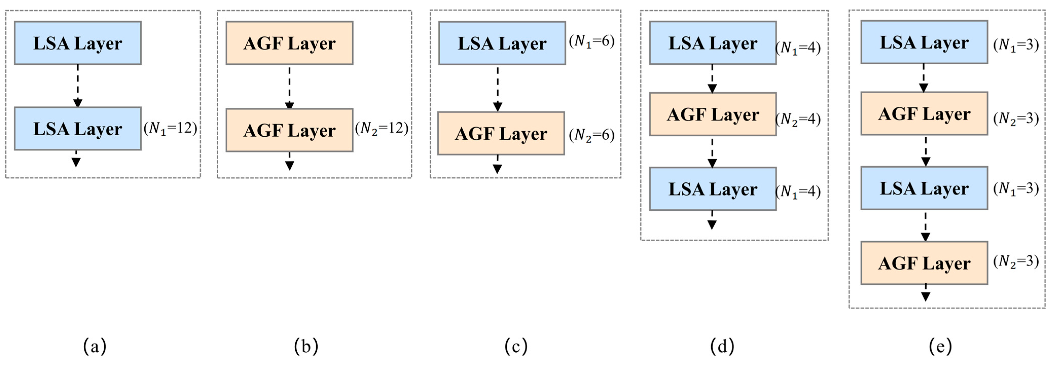
Following the initial ablation study on the AWF and AGF modules, we further investigated the architectural design of the model by exploring different stacking strategies and quantities of the LSA and AGF layers. As shown in Figure 11, six configurations (a)–(e) were evaluated, each representing a distinct way of organizing the LSA and AGF layers in the encoder. To ensure a fair comparison, all other components of the architecture were kept unchanged.
Table 6 analysis reveals that varying LSA layer architectures produce measurable differences in system performance metrics. (a) and (b), which stack only LSA layers or only AGF layers, respectively, exhibit relatively lower overall performance. This indicates that relying solely on a single type of module is insufficient for effectively extracting and fusing multi-modal feature information. (c) adopts a sequential stacking approach, where LSA and AGF layers are arranged one after another. Its performance improves significantly compared to the previous two, demonstrating that the combination of the two mechanisms enhances feature representation capabilities. (d) further interleaves LSA and AGF layers, allowing for tighter integration between attention-based modeling and modality fusion, resulting in another performance boost. (e), which employs a more compact interleaved stacking strategy with an equal number of LSA and AGF layers ( N 1 = N 2 = 3), achieves the best results across all three metrics: OA, mF1, and mIoU. This configuration not only maintains computational efficiency but also significantly enhances feature extraction and fusion accuracy, achieving an ideal balance between global modeling and local detail refinement.
In addition to the quantitative comparison, we also conducted a brief qualitative examination of the segmentation outcomes under different stacking configurations. We observed that configurations (a)–(d) tend to produce varying degrees of boundary discontinuity or small-object omission, especially in regions with fine-grained structures. In contrast, configuration (e) yields more coherent boundaries and better preserves small targets, indicating a more balanced integration of local detail modeling and global semantic fusion. These qualitative observations are consistent with the quantitative improvements reported in Table 6.
To further evaluate the robustness of the LSA module, we conducted a sensitivity analysis on the Top-K sparsity ratio k. As shown in Table 7, we tested three sparsity levels (10%, 20%, 30%) on the Vaihingen dataset while keeping all other model settings fixed. The results indicate that k = 20% yields the highest segmentation accuracy. A smaller sparsity (10%) excessively prunes useful attention responses, whereas a larger sparsity (30%) weakens the selective sparsification effect. Therefore, selecting k = 20% achieves the best trade-off between sparse attention modeling and segmentation performance.

4.6. Computational Complexity Analysis

To further evaluate the efficiency and effectiveness of the proposed model, we compare its computational complexity and segmentation performance against several representative methods. Specifically, we report three key metrics: the number of floating-point operations (FLOPs), the total number of trainable parameters, and mIoU.
In the calculation of GFLOPs, we used a 256 × 256 input patch size, which is consistent during both the training and inference stages. The GFLOPs calculation is based on the number of floating-point operations performed during each inference.
Table 8 presents the complexity analysis results for several typical methods. It can be observed that, despite having more parameters, the proposed ASGT-Net model has significantly lower FLOPs compared to most other models, while also achieving excellent segmentation accuracy. This indicates that ASGT-Net effectively improves model performance while maintaining low computational overhead.
Additionally, we evaluated the inference throughput (FPS) of ASGT-Net, which is approximately 65 frames per second during inference, demonstrating high real-time processing capability. The maximum GPU memory usage during inference is approximately 14 GB, which may present some memory challenges in resource-constrained environments. During training, the average time per epoch is about 12 s, indicating high training efficiency.
The reduced FLOPs can lead to faster inference times, making ASGT-Net more suitable for real-time applications, where processing speed is crucial, such as in operational remote sensing systems. However, the high parameter count could present memory challenges, especially in environments with limited hardware resources. Therefore, the trade-off between inference speed and memory usage should be considered when deploying the model in different contexts.

5. Conclusions

In conclusion, this study proposes ASGT-Net, a multi-modal fusion network that achieves high-performance semantic segmentation through a strategically designed symmetric dual-branch encoder. At the shallow layers, AWF balances the contributions from different modalities, while at the deeper layers, the synergy between LSA and AGF establishes a balance between global contextual understanding and local detail focus. Experimental results demonstrate that this symmetric dual-branch framework excels in segmenting complex scenes, with the synergistic symmetry of its components being critical for achieving robust performance and an optimal trade-off between accuracy and efficiency.
A series of experiments have demonstrated the superior qualities of our custom-built network for segmenting remote sensing images semantically. Compared to traditional multi-modal fusion methods, the proposed approach achieves superior segmentation accuracy in complex scenes such as buildings, low vegetation, trees, and small targets. Ablation experiments reveal that removing either the adaptive weighted fusion or Learnable Sparse Attention mechanisms significantly reduces the model’s segmentation accuracy, highlighting the critical role of these components in enhancing performance. Additionally, based on the analysis of computational complexity, the proposed network achieves a good balance between accuracy and computational efficiency.
Although ASGT-Net has made significant progress in multi-modal fusion and remote sensing image semantic segmentation tasks, future research should focus on improving the model’s performance in handling small-scale targets, particularly in complex backgrounds or when targets are partially occluded. As the resolution of remote sensing images increases, the demand for processing ultra-high-resolution images also grows, which could lead to memory and computational resource bottlenecks, especially in environments with limited hardware resources. Therefore, future work should optimize memory management and computational efficiency or develop more efficient hardware acceleration techniques to address the demands of processing large-scale remote sensing data. Current experiments have primarily focused on urban scenes (Vaihingen and Potsdam datasets), but future research should extend to rural, forest, and water body environments to validate ASGT-Net’s adaptability in various remote sensing tasks. Additionally, future work will further refine the Learnable Sparse Attention (LSA) mechanism to enhance its efficiency in large-scale datasets, particularly in balancing the capture of local details and long-range dependencies, while also improving the adaptability and flexibility of the AGF module to handle data fusion in dynamic scenes. With the increasing richness of remote sensing data, hyperspectral imagery holds great potential for applications such as agricultural land cover mapping. Future research will explore the application of ASGT-Net in such tasks, analyzing how multi-modal data can collaborate to improve the model’s robustness and generalization ability.

Author Contributions

Conceptualization, W.Y. and W.C.; methodology, W.Y. and K.C.; software, X.L.; validation, W.Y., K.C. and X.L.; formal analysis, W.Y.; investigation, W.Y.; resources, K.T.; data curation, W.Y.; writing—original draft preparation, W.Y.; writing—review and editing, W.C.; visualization, K.C.; supervision, W.C.; project administration, W.C.; funding acquisition, W.C. All authors have read and agreed to the published version of the manuscript.

Funding

This work was supported by the autonomous deployment project of the Xinjiang Institute of Ecology and Geography, Chinese Academy of Sciences (E5508502, B2-2023-0239), grants from the Xinjiang Uyghur Autonomous Region’s Science and Technology Assistance Program (2024E02028), and the Shandong Natural Science Youth Foundation (ZR2023QD070).

Data Availability Statement

All data used in this study are publicly available from the ISPRS Vaihingen and Potsdam datasets.

Acknowledgments

We deeply appreciate the constructive feedback provided by the editors and anonymous peer reviewers.

Conflicts of Interest

The authors declare no conflicts of interest. The funders had no role in the design of the study; in the collection, analyses, or interpretation of data; in the writing of the manuscript; or in the decision to publish the results.

References

  1. Richards, J.A.; Richards, J.A. Remote Sensing Digital Image Analysis; Springer: Cham, Switzerland, 2022; Volume 5. [Google Scholar]
  2. Teixeira, A.C.; Bakon, M.; Lopes, D.; Cunha, A.; Sousa, J.J. A systematic review on soil moisture estimation using remote sensing data for agricultural applications. Sci. Remote Sens. 2025, 12, 100328. [Google Scholar] [CrossRef]
  3. Du, P.; Xia, J.S.; Xue, Z.H.; Tan, K.; Su, H.; Bao, R. Review of hyperspectral remote sensing image classification. J. Remote Sens. 2016, 20, 236–256. [Google Scholar] [CrossRef]
  4. Cheng, J.; Deng, C.; Su, Y.; An, Z.; Wang, Q. Methods and datasets on semantic segmentation for Unmanned Aerial Vehicle remote sensing images: A review. ISPRS J. Photogramm. Remote Sens. 2024, 211, 1–34. [Google Scholar] [CrossRef]
  5. Adam, J.M.; Liu, W.; Zang, Y.; Afzal, M.K.; Bello, S.A.; Muhammad, A.U.; Wang, C.; Li, J. Deep learning-based semantic segmentation of urban-scale 3D meshes in remote sensing: A survey. Int. J. Appl. Earth Obs. Geoinf. 2023, 121, 103365. [Google Scholar] [CrossRef]
  6. Jia, P.; Chen, C.; Zhang, D.; Sang, Y.; Zhang, L. Semantic segmentation of deep learning remote sensing images based on band combination principle: Application in urban planning and land use. Comput. Commun. 2024, 217, 97–106. [Google Scholar] [CrossRef]
  7. Jin, C.; Zhou, L.; Zhao, Y.; Qi, H.; Wu, X.; Zhang, C. Classification of rice varieties using hyperspectral imaging with multi-dimensional fusion convolutional neural networks. J. Food Compos. Anal. 2025, 148, 108389. [Google Scholar] [CrossRef]
  8. Ma, L.; Liu, Y.; Zhang, X.; Ye, Y.; Yin, G.; Johnson, B.A. Deep learning in remote sensing applications: A meta-analysis and review. ISPRS J. Photogramm. Remote Sens. 2019, 152, 166–177. [Google Scholar] [CrossRef]
  9. Bhatti, M.A.; Syam, M.S.; Chen, H.; Hu, Y.; Keung, L.W.; Zeeshan, Z.; Ali, Y.A.; Sarhan, N. Utilizing convolutional neural networks (CNN) and U-Net architecture for precise crop and weed segmentation in agricultural imagery: A deep learning approach. Big Data Res. 2024, 36, 100465. [Google Scholar] [CrossRef]
  10. Lee, G.; Shin, J.; Kim, H. VFF-Net: Evolving forward–forward algorithms into convolutional neural networks for enhanced computational insights. Neural Netw. 2025, 190, 107697. [Google Scholar] [CrossRef]
  11. Abdulgalil, H.D.; Basir, O.A. Next-generation image captioning: A survey of methodologies and emerging challenges from transformers to Multimodal Large Language Models. Nat. Lang. Process. J. 2025, 12, 100159. [Google Scholar] [CrossRef]
  12. Thirunavukarasu, R.; Kotei, E. A comprehensive review on transformer network for natural and medical image analysis. Comput. Sci. Rev. 2024, 53, 100648. [Google Scholar] [CrossRef]
  13. Wang, Z.; Li, J.; Xu, N.; You, Z. Combining feature compensation and GCN-based reconstruction for multimodal remote sensing image semantic segmentation. Inf. Fusion 2025, 122, 103207. [Google Scholar] [CrossRef]
  14. Fan, Y.; Qian, Y.; Gong, W.; Chu, Z.; Qin, Y.; Muhetaer, P. Multi-level interactive fusion network based on adversarial learning for fusion classification of hyperspectral and LiDAR data. Expert Syst. Appl. 2024, 257, 125132. [Google Scholar] [CrossRef]
  15. Geng, Z.; Liu, H.; Duan, P.; Wei, X.; Li, S. Feature-based multimodal remote sensing image matching: Benchmark and state-of-the-art. ISPRS J. Photogramm. Remote Sens. 2025, 229, 285–302. [Google Scholar] [CrossRef]
  16. Li, J.; Hong, D.; Gao, L.; Yao, J.; Zheng, K.; Zhang, B.; Chanussot, J. Deep learning in multimodal remote sensing data fusion: A comprehensive review. Int. J. Appl. Earth Obs. Geoinf. 2022, 112, 102926. [Google Scholar] [CrossRef]
  17. Dalla Mura, M.; Prasad, S.; Pacifici, F.; Gamba, P.; Chanussot, J.; Benediktsson, J.A. Challenges and opportunities of multimodality and data fusion in remote sensing. Proc. IEEE 2015, 103, 1585–1601. [Google Scholar] [CrossRef]
  18. Zubair, M.; Hussain, M.; Albashrawi, M.A.; Bendechache, M.; Owais, M. A comprehensive review of techniques, algorithms, advancements, challenges, and clinical applications of multi-modal medical image fusion for improved diagnosis. Comput. Methods Programs Biomed. 2025, 272, 109014. [Google Scholar] [CrossRef]
  19. Zhang, Y.; Wang, Z.; Huang, M.; Li, M.; Zhang, J.; Wang, S.; Zhang, J.; Zhang, H. S2DBFT: Spectral-Spatial Dual-Branch Fusion Transformer for Hyperspectral Image Classification. IEEE Trans. Geosci. Remote Sens. 2025, 63, 5525517. [Google Scholar] [CrossRef]
  20. Aleissaee, A.A.; Kumar, A.; Anwer, R.M.; Khan, S.; Cholakkal, H.; Xia, G.-S.; Khan, F.S. Transformers in remote sensing: A survey. Remote Sens. 2023, 15, 1860. [Google Scholar] [CrossRef]
  21. Wang, R.; Ma, L.; He, G.; Johnson, B.A.; Yan, Z.; Chang, M.; Liang, Y. Transformers for Remote Sensing: A Systematic Review and Analysis. Sensors 2024, 24, 3495. [Google Scholar] [CrossRef]
  22. Wu, S.; Wu, T.; Lin, F.; Tian, S.; Guo, G. Fully transformer networks for semantic image segmentation. arXiv 2021, arXiv:2106.04108. [Google Scholar] [CrossRef]
  23. Ajibola, S.; Cabral, P. A Systematic Literature Review and Bibliometric Analysis of Semantic Segmentation Models in Land Cover Mapping. Remote Sens. 2024, 16, 2222. [Google Scholar] [CrossRef]
  24. Chen, L.-C.; Zhu, Y.; Papandreou, G.; Schroff, F.; Adam, H. Encoder-decoder with atrous separable convolution for semantic image segmentation. In Proceedings of the European Conference on Computer Vision (ECCV), Munich, Germany, 8–14 September 2018; pp. 801–818. [Google Scholar]
  25. Ronneberger, O.; Fischer, P.; Brox, T. U-net: Convolutional networks for biomedical image segmentation. In Proceedings of the Medical Image Computing and Computer-Assisted Intervention—MICCAI 2015: 18th International Conference, Munich, Germany, 5–9 October 2015; Proceedings, Part III 18. pp. 234–241. [Google Scholar]
  26. Badrinarayanan, V.; Kendall, A.; Cipolla, R. Segnet: A deep convolutional encoder-decoder architecture for image segmentation. IEEE Trans. Pattern Anal. Mach. Intell. 2017, 39, 2481–2495. [Google Scholar] [CrossRef]
  27. Noh, H.; Hong, S.; Han, B. Learning deconvolution network for semantic segmentation. In Proceedings of the IEEE International Conference on Computer Vision, Santiago, Chile, 7–13 December 2015; pp. 1520–1528. [Google Scholar]
  28. Dosovitskiy, A. An image is worth 16x16 words: Transformers for image recognition at scale. arXiv 2020, arXiv:2010.11929. [Google Scholar]
  29. Zheng, S.; Lu, J.; Zhao, H.; Zhu, X.; Luo, Z.; Wang, Y.; Fu, Y.; Feng, J.; Xiang, T.; Torr, P.H. Rethinking semantic segmentation from a sequence-to-sequence perspective with transformers. In Proceedings of the IEEE/CVF Conference on Computer Vision and Pattern Recognition, Virtual, 19–25 June 2021; pp. 6881–6890. [Google Scholar]
  30. Strudel, R.; Garcia, R.; Laptev, I.; Schmid, C. Segmenter: Transformer for semantic segmentation. In Proceedings of the IEEE/CVF International Conference on Computer Vision, Virtual, 11–17 October 2021; pp. 7262–7272. [Google Scholar]
  31. Tang, H.; Zeng, K. Remote Sensing Image Information Granulation Transformer for Semantic Segmentation. Comput. Mater. Contin. 2025, 84, 1485–1506. [Google Scholar] [CrossRef]
  32. Ni, Y.; Xue, D.; Chi, W.; Luan, J.; Liu, J. CSFAFormer: Category-selective feature aggregation transformer for multimodal remote sensing image semantic segmentation. Inf. Fusion 2025, 127, 103786. [Google Scholar] [CrossRef]
  33. Liu, Y.; Gao, K.; Wang, H.; Yang, Z.; Wang, P.; Ji, S.; Huang, Y.; Zhu, Z.; Zhao, X. A Transformer-based multi-modal fusion network for semantic segmentation of high-resolution remote sensing imagery. Int. J. Appl. Earth Obs. Geoinf. 2024, 133, 104083. [Google Scholar] [CrossRef]
  34. Wang, W.; Xie, E.; Li, X.; Fan, D.-P.; Song, K.; Liang, D.; Lu, T.; Luo, P.; Shao, L. Pyramid vision transformer: A versatile backbone for dense prediction without convolutions. In Proceedings of the IEEE/CVF International Conference on Computer Vision, Virtual, 11–17 October 2021; pp. 568–578. [Google Scholar]
  35. Liu, Z.; Lin, Y.; Cao, Y.; Hu, H.; Wei, Y.; Zhang, Z.; Lin, S.; Guo, B. Swin transformer: Hierarchical vision transformer using shifted windows. In Proceedings of the IEEE/CVF International Conference on Computer Vision, Virtual, 11–17 October 2021; pp. 10012–10022. [Google Scholar]
  36. Xie, E.; Wang, W.; Yu, Z.; Anandkumar, A.; Alvarez, J.M.; Luo, P. SegFormer: Simple and efficient design for semantic segmentation with transformers. In Proceedings of the 35th International Conference on Neural Information Processing Systems, Online, 6–14 December 2021; Article 924. [Google Scholar]
  37. Child, R.; Gray, S.; Radford, A.; Sutskever, I. Generating Long Sequences with Sparse Transformers. arXiv 2019, arXiv:1904.10509. [Google Scholar] [CrossRef]
  38. Beltagy, I.; Peters, M.E.; Cohan, A. Longformer: The long-document transformer. arXiv 2020, arXiv:2004.05150. [Google Scholar] [CrossRef]
  39. Zaheer, M.; Guruganesh, G.; Dubey, K.A.; Ainslie, J.; Alberti, C.; Ontanon, S.; Pham, P.; Ravula, A.; Wang, Q.; Yang, L. Big bird: Transformers for longer sequences. Adv. Neural Inf. Process. Syst. 2020, 33, 17283–17297. [Google Scholar]
  40. Yuan, Y.; Fu, R.; Huang, L.; Lin, W.; Zhang, C.; Chen, X.; Wang, J. Hrformer: High-resolution transformer for dense prediction. arXiv 2021, arXiv:2110.09408. [Google Scholar] [CrossRef]
  41. Zhou, Z.; Siddiquee, M.M.R.; Tajbakhsh, N.; Liang, J. Unet++: Redesigning skip connections to exploit multiscale features in image segmentation. IEEE Trans. Med. Imaging 2019, 39, 1856–1867. [Google Scholar] [CrossRef]
  42. Ranftl, R.; Bochkovskiy, A.; Koltun, V. Vision transformers for dense prediction. In Proceedings of the IEEE/CVF International Conference on Computer Vision, Virtual, 11–17 October 2021; pp. 12179–12188. [Google Scholar]
  43. Valada, A.; Oliveira, G.L.; Brox, T.; Burgard, W. Deep multispectral semantic scene understanding of forested environments using multimodal fusion. In Proceedings of the 2016 International Symposium on Experimental Robotics, Tokyo, Japan, 3–6 October 2016; pp. 465–477. [Google Scholar]
  44. Qi, C.R.; Yi, L.; Su, H.; Guibas, L.J. Pointnet++: Deep hierarchical feature learning on point sets in a metric space. In Advances in Neural Information Processing Systems; MIT Press: Cambridge, MA, USA, 2017; Volume 30. [Google Scholar]
  45. Hazirbas, C.; Ma, L.; Domokos, C.; Cremers, D. Fusenet: Incorporating depth into semantic segmentation via fusion-based cnn architecture. In Proceedings of the Computer Vision—ACCV 2016: 13th Asian Conference on Computer Vision, Taipei, Taiwan, 20–24 November 2016; Revised Selected Papers, Part I 13. pp. 213–228. [Google Scholar]
  46. Roy, S.K.; Deria, A.; Hong, D.; Rasti, B.; Plaza, A.; Chanussot, J. Multimodal fusion transformer for remote sensing image classification. IEEE Trans. Geosci. Remote Sens. 2023, 61, 5515620. [Google Scholar] [CrossRef]
  47. Baltrušaitis, T.; Ahuja, C.; Morency, L.-P. Multimodal machine learning: A survey and taxonomy. IEEE Trans. Pattern Anal. Mach. Intell. 2018, 41, 423–443. [Google Scholar] [CrossRef]
  48. Valada, A.; Mohan, R.; Burgard, W. Self-supervised model adaptation for multimodal semantic segmentation. Int. J. Comput. Vis. 2020, 128, 1239–1285. [Google Scholar] [CrossRef]
  49. Wang, N.; Wu, Q.; Gui, Y.; Hu, Q.; Li, W. Cross-Modal Segmentation Network for Winter Wheat Mapping in Complex Terrain Using Remote-Sensing Multi-Temporal Images and DEM Data. Remote Sens. 2024, 16, 1775. [Google Scholar] [CrossRef]
  50. Woo, S.; Park, J.; Lee, J.-Y.; Kweon, I.S. Cbam: Convolutional block attention module. In Proceedings of the European Conference on Computer Vision (ECCV), Munich, Germany, 8–14 September 2018; pp. 3–19. [Google Scholar]
  51. Zhang, B.; Ming, Z.; Feng, W.; Liu, Y.; He, L.; Zhao, K. MMFormer: Multimodal Transformer Using Multiscale Self-Attention for Remote Sensing Image Classification. arXiv 2023, arXiv:2303.13101. [Google Scholar] [CrossRef]
  52. Ibtehaz, N.; Rahman, M.S. MultiResUNet: Rethinking the U-Net architecture for multimodal biomedical image segmentation. Neural Netw. 2020, 121, 74–87. [Google Scholar] [CrossRef]
  53. Schneider, L.; Jasch, M.; Fröhlich, B.; Weber, T.; Franke, U.; Pollefeys, M.; Rätsch, M. Multimodal neural networks: RGB-D for semantic segmentation and object detection. In Proceedings of the Image Analysis: 20th Scandinavian Conference, SCIA 2017, Tromsø, Norway, 12–14 June 2017; Proceedings, Part I 20. pp. 98–109. [Google Scholar]
  54. Hu, C.; Zhao, C.; Shao, H.; Deng, J.; Wang, Y. TMFF: Trustworthy multi-focus fusion framework for multi-label sewer defect classification in sewer inspection videos. IEEE Trans. Circuits Syst. Video Technol. 2024, 34, 12274–12287. [Google Scholar] [CrossRef]
  55. Du, Y.; Liu, Y.; Peng, Z.; Jin, X. Gated attention fusion network for multimodal sentiment classification. Knowl.-Based Syst. 2022, 240, 108107. [Google Scholar] [CrossRef]
  56. Arevalo, J.; Solorio, T.; Montes-y-Gomez, M.; González, F.A. Gated multimodal networks. Neural Comput. Appl. 2020, 32, 10209–10228. [Google Scholar] [CrossRef]
  57. Cao, B.; Sun, Y.; Zhu, P.; Hu, Q. Multi-modal gated mixture of local-to-global experts for dynamic image fusion. In Proceedings of the IEEE/CVF International Conference on Computer Vision, Paris, France, 1–6 October 2023; pp. 23555–23564. [Google Scholar]
  58. Kim, J.; Koh, J.; Kim, Y.; Choi, J.; Hwang, Y.; Choi, J.W. Robust deep multi-modal learning based on gated information fusion network. In Proceedings of the Asian Conference on Computer Vision, Perth, Australia, 2–6 December 2018; pp. 90–106. [Google Scholar]
  59. Chen, X.; Lin, K.-Y.; Wang, J.; Wu, W.; Qian, C.; Li, H.; Zeng, G. Bi-directional cross-modality feature propagation with separation-and-aggregation gate for RGB-D semantic segmentation. In Proceedings of the European Conference on Computer Vision, Glasgow, UK, 23–28 August 2020; pp. 561–577. [Google Scholar]
  60. Shen, Z.; He, Y.; Du, X.; Yu, J.; Wang, H.; Wang, Y. YCANet: Target detection for complex traffic scenes based on camera-LiDAR fusion. IEEE Sens. J. 2024, 24, 8379–8389. [Google Scholar] [CrossRef]
  61. Zhou, G.; Zhi, H.; Gao, E.; Lu, Y.; Chen, J.; Bai, Y.; Zhou, X. DeepU-Net: A Parallel Dual-Branch Model for Deeply Fusing Multi-Scale Features for Road Extraction from High-Resolution Remote Sensing Images. IEEE J. Sel. Top. Appl. Earth Obs. Remote Sens. 2025, 18, 9448–9463. [Google Scholar] [CrossRef]
  62. Li, R.; Zheng, S.; Zhang, C.; Duan, C.; Wang, L.; Atkinson, P.M. ABCNet: Attentive bilateral contextual network for efficient semantic segmentation of Fine-Resolution remotely sensed imagery. ISPRS J. Photogramm. Remote Sens. 2021, 181, 84–98. [Google Scholar] [CrossRef]
  63. Zhao, H.; Shi, J.; Qi, X.; Wang, X.; Jia, J. Pyramid scene parsing network. In Proceedings of the IEEE Conference on Computer Vision and Pattern Recognition, Honolulu, HI, USA, 21–26 July 2017; pp. 2881–2890. [Google Scholar]
  64. Audebert, N.; Le Saux, B.; Lefèvre, S. Beyond RGB: Very high resolution urban remote sensing with multimodal deep networks. ISPRS J. Photogramm. Remote Sens. 2018, 140, 20–32. [Google Scholar] [CrossRef]
  65. Seichter, D.; Köhler, M.; Lewandowski, B.; Wengefeld, T.; Gross, H.-M. Efficient rgb-d semantic segmentation for indoor scene analysis. In Proceedings of the 2021 IEEE International Conference on Robotics and Automation (ICRA), Xi’an, China, 30 May–5 June 2021; pp. 13525–13531. [Google Scholar]
  66. Hosseinpour, H.; Samadzadegan, F.; Javan, F.D. CMGFNet: A deep cross-modal gated fusion network for building extraction from very high-resolution remote sensing images. ISPRS J. Photogramm. Remote Sens. 2022, 184, 96–115. [Google Scholar] [CrossRef]
  67. Chen, J.; Lu, Y.; Yu, Q.; Luo, X.; Adeli, E.; Wang, Y.; Lu, L.; Yuille, A.L.; Zhou, Y. Transunet: Transformers make strong encoders for medical image segmentation. arXiv 2021, arXiv:2102.04306. [Google Scholar] [CrossRef]
  68. Wang, L.; Li, R.; Zhang, C.; Fang, S.; Duan, C.; Meng, X.; Atkinson, P.M. UNetFormer: A UNet-like transformer for efficient semantic segmentation of remote sensing urban scene imagery. ISPRS J. Photogramm. Remote Sens. 2022, 190, 196–214. [Google Scholar] [CrossRef]
  69. Ma, X.; Zhang, X.; Pun, M.-O. A crossmodal multiscale fusion network for semantic segmentation of remote sensing data. IEEE J. Sel. Top. Appl. Earth Obs. Remote Sens. 2022, 15, 3463–3474. [Google Scholar] [CrossRef]
  70. He, S.; Yang, H.; Zhang, X.; Li, X. MFTransNet: A multi-modal fusion with CNN-transformer network for semantic segmentation of HSR remote sensing images. Mathematics 2023, 11, 722. [Google Scholar] [CrossRef]
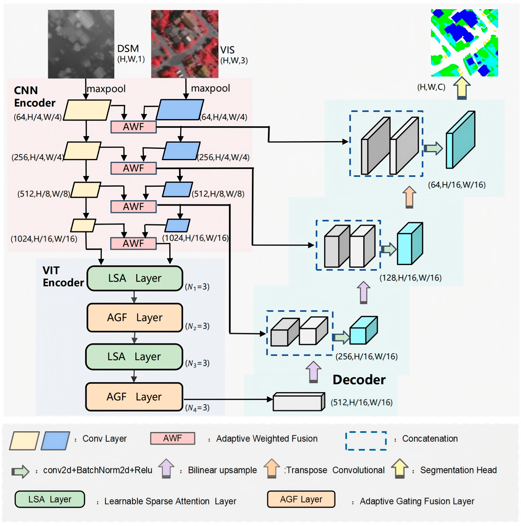
Figure 1. Overall architecture of ASGT-Net, which consists of three main components: a CNN encoder, a ViT encoder, and a decoder. The CNN encoder extracts and fuses multi-scale VIS and DSM features using convolutional layers and the AWF module. The ViT encoder models local sparse attention and global context by alternately stacking LSA and AGF blocks. The decoder progressively restores spatial resolution and combines multi-scale features to produce the final segmentation map.
Symmetry 17 02070 g001
Figure 2. The schematic representation of the AWF layer is depicted. This layer accomplishes adaptive fusion by computing attention weights for both DSM and VIS features, and then performing a weighted summation based on these weights.
Symmetry 17 02070 g002
Figure 3. Structure of the proposed LSA block, which inserts a local sparse attention module into a standard Transformer block with a feed-forward network, residual connections, and layer normalization.
Symmetry 17 02070 g003
Figure 4. Computation flow of LSA: the input X is projected into Q, K, and V, sparse attention is applied, followed by softmax normalization and a linear projection to obtain the output.
Symmetry 17 02070 g004
Figure 5. Illustration of the AGF layer. Its architecture resembles that of the LSA layer.
Symmetry 17 02070 g005
Figure 6. Details of the AGF module. The input features undergo self-attention, followed by linear transformations and Sigmoid activation to generate adaptive weights. These adaptive weights are then utilized in a process involving element-wise multiplication and summation to derive the final fused output.
Symmetry 17 02070 g006
Figure 7. The data samples comprised RGB, DSM, and Ground Truth (GT) are derived from the ISPRS Vaihingen and Potsdam datasets. Specifically, (a) presents samples from the Vaihingen dataset, whereas (b) showcases samples from the Potsdam dataset.
Symmetry 17 02070 g007
Figure 8. The performance comparison between SA-GATE, TransUNet, MFTransNet, CMFNet, and the proposed ASGT-Net on the Vaihingen dataset, with boxes indicating segmentation differences.
Symmetry 17 02070 g008
Figure 9. The performance comparison between SA-GATE, TransUNet, MFTransNet, CMFNet, and the proposed ASGT-Net on the Potsdam dataset, with boxes indicating segmentation differences.
Symmetry 17 02070 g009
Figure 10. Compares the baseline, AWF, SGF, and ASGT-Net on the Vaihingen dataset, with boxes highlighting segmentation differences.
Symmetry 17 02070 g010
Figure 11. Five different configurations (ae) were constructed, with each configuration representing a distinct way of organizing the LSA and AGF layers in the encoder. N 1 represents the number of LSA layers, N 2 denotes the number of AGF layers.
Symmetry 17 02070 g011
Table 1. Training hyperparameters used in all experiments.
HyperparameterValue
Batch size10
Epochs50
OptimizerSGD
Initial learning rate0.01
Momentum0.9
Weight decay0.0005
LR schedulerMultiStepLR
LR decay milestones[25, 35, 45]
LR decay factor γ0.1
Loss functionWeighted Cross-Entropy
Sparsity learning rate0.001
Sparsity LR schedulerMultiStepLR (same milestones)
L1 regularization λ1 × 10⁻⁴
Early stopping patience7
Early stopping min delta0.001
Random seed42
Table 2. Outcomes from Tests Using the Vaihingen Dataset.
MethodOA(%)mF1 (%)mIoU (%)
Impervious SurfacesBuildingLow
Vegetation
TreeCarTotal
ABCNet (2021) [62] (ABCNet—https://github.com/lironui/ABCNet (commit: 3067b46; accessed on 26 October 2025))94.1090.8178.5364.1289.7089.2585.3475.20
PSPNet (2017) [63] (PSPNet—https://github.com/hszhao/PSPNet (commit: 798bdc9; accessed on 26 October 2025)94.5290.1778.8479.2292.0389.9486.5576.96
FuseNet (2016) [45] (FuseNet—https://github.com/xmindflow/FuseNet (commit: e8ec1b4; accessed on 26 October 2025)96.2890.2878.9881.3791.6690.5187.7178.71
vFuseNet (2018) [64]95.9291.3677.6476.0691.8590.4987.8978.92
ESANet (2021) [65] (ESANet—https://github.com/TUI-NICR/ESANet (commit: 49d2201; accessed on 26 October 2025))95.6990.5077.1685.4691.3990.6188.1879.42
CMGFNet (2022) [66] (CMGFNet—https://github.com/hamidreza2015/CMGFNet-Building_Extraction (commit: e0ce252; accessed on 26 October 2025))97.7591.6080.0387.2892.3591.7290.0082.26
SA-GATE (2020) [59] (SA-GATE—https://github.com/charlesCXK/RGBD_Semantic_Segmentation_PyTorch (commit: 32b3f86; accessed on 26 October 2025))91.6994.8481.2992.5687.7991.1089.8181.27
TransUNet (2021) [67] (TransUNet—https://github.com/Beckschen/TransUNet (commit: 192e441; accessed on 26 October 2025))91.6696.4876.1492.7769.5690.9687.3478.26
UNetFormer (2022) [68] (UNetFormer—https://github.com/WangLibo1995/GeoSeg (commit: 9453fe4; accessed on 26 October 2025))97.6986.4787.9395.9192.2790.6589.8581.97
CMFNet (2022) [69] (CMFNet—https://github.com/FanChiMao/CMFNet (commit: 84a05e1; accessed on 26 October 2025))92.3697.1780.3790.8285.4791.4089.4881.44
MFTransNet (2023) [70]92.1196.41 80.0991.4886.5291.2289.6281.61
ASGT-Net92.4897.7682.1891.7390.3392.3090.8883.65
Table 3. Outcomes of Tests Conducted Using the Potsdam Dataset.
MethodOA(%)mF1 (%)mIoU (%)
Impervious SurfacesBuildingLow
Vegetation
TreeCarTotal
ABCNet (2021) [62]88.9096.2386.4078.9292.9287.5288.1479.26
PSPNet (2017) [63]90.9197.0385.6783.1388.8188.6788.9280.36
FuseNet (2016) [45]92.6497.4887.3185.1496.1090.5891.6084.86
vFuseNet (2018) [64]91.6291.3689.0384.2995.4990.2287.8978.92
ESANet (2021) [65]92.7697.1087.8185.3194.0890.6188.1879.42
CMGFNet (2022) [66]92.6097.4186.6886.8095.6889.7491.4084.53
SA-GATE (2020) [59]90.7796.5485.3581.1896.6387.9190.2682.53
TransUNet (2021) [67]91.9396.6389.9882.6593.1790.0190.9783.74
UNetFormer (2022) [68]92.2797.6987.9395.9195.9190.6591.7185.05
CMFNet (2022) [69]92.8497.6388.0086.4795.6891.1692.1085.63
MFTransNet (2023) [70]92.4597.3786.9285.7196.0589.9691.1184.04
ASGT-Net92.8998.2489.2091.3694.0291.2492.3086.10
Table 4. Per-seed performance of ASGT-Net on the Vaihingen and Potsdam datasets.
DatasetSeedOA(%)mF1 (%)mIoU (%)
Vaihingen4291.3492.5186.32
Vaihingen340791.2792.4886.10
Vaihingen202591.4192.4986.25
Vaihingen (Mean ± Std)91.34 ± 0.0792.49 ± 0.0286.22 ± 0.09
Potsdam4291.2892.3386.12
Potsdam340791.1992.2786.05
Potsdam202591.2592.3086.14
Potsdam (Mean ± Std)91.24 ± 0.0492.30 ± 0.0386.10 ± 0.04
Table 5. Comparison Of Different Methods Based On AWF And AGF Performance.
MethodAWFAGFOA(%)mF1 (%)mIoU (%)Impervious Surfaces
IoU (%)
Building
IoU (%)
Low Vegetation
IoU (%)
Tree
IoU (%)
Car
IoU (%)
Baseline 90.9687.3478.2682.085.577.276.374.5
Ours 92.1690.5483.1387.589.082.781.078.3
Ours 91.4690.2982.6386.388.281.979.577.8
Ours92.3090.8883.6588.089.383.281.578.8
Table 6. Performance Comparison Under Different Configurations of LSA And AGF Layer Stacking.
StructureOA(%)mF1 (%)mIoU (%)Impervious Surfaces
IoU (%)
Building
IoU (%)
Low Vegetation
IoU (%)
Tree
IoU (%)
Car
IoU (%)
(a)90.3788.8980.4681.885.076.575.873.5
(b)89.7588.8280.1986.588.282.080.577.0
(c)91.5489.8782.0285.887.581.278.876.5
(d)91.7790.0982.4387.588.782.880.577.8
(e)92.3090.8883.6588.089.583.581.578.5
Table 7. Sensitivity analysis of different Top-K sparsity ratios k in the LSA module.
Top-K Ratio (k)mIoU (%)
10%82.75
20%83.65
30%83.02
Table 8. Computational Complexity and Segmentation Performance Comparison.
MethodParameters (M)GFLOPs(G)mIoU (%)
PSPNet (2017) [63]46.7249.0376.96
FuseNet (2016) [45]42.0858.3778.71
vFuseNet (2018) [64]44.1760.3678.92
SA-GATE (2020) [59]110.8541.2881.27
CMFNet (2022) [69]123.6378.2581.44
MFTransNet (2023) [70]130.5055.6082.10
ASGT-Net150.3948.8783.65
Disclaimer/Publisher’s Note: The statements, opinions and data contained in all publications are solely those of the individual author(s) and contributor(s) and not of MDPI and/or the editor(s). MDPI and/or the editor(s) disclaim responsibility for any injury to people or property resulting from any ideas, methods, instructions or products referred to in the content.