Article

Prescribed Performance Adaptive Fault-Tolerant Control for Nonlinear System with Actuator Faults and Dead Zones

by
Zhenlin Wang
1,
Seiji Hashimoto
1,*,
Nobuyuki Kurita
2,
Pengqiang Nie
1,
Song Xu
3 and
Takahiro Kawaguchi
1
1
Division of Electronics and Informatics, Gunma University, Kiryu 376-8515, Japan
2
Department of Surgery, Baylor College of Medicine, 1 Baylor Plz, Houston, TX 77030, USA
3
College of Automation, Jiangsu University of Science and Technology, Zhenjiang 212000, China
*
Author to whom correspondence should be addressed.
Symmetry 2025, 17(11), 1915; https://doi.org/10.3390/sym17111915
Submission received: 28 August 2025 / Revised: 18 October 2025 / Accepted: 31 October 2025 / Published: 8 November 2025
(This article belongs to the Section Mathematics)

Abstract

This study proposes an adaptive fault-tolerant control strategy for parametric strict-feedback systems subject to actuator faults and unknown dead-zone nonlinearities, a combination that presents significant challenges for controller design. First, a novel prescribed-performance fault-tolerant control framework is developed by incorporating a funnel function, a barrier Lyapunov function, and a bounded estimation mechanism to address the issue of multiple constrained nonlinear disturbances. Second, the proposed strategy offers two key improvements: (1) adequate compensation for the coupled effects of actuator faults and dead-zone nonlinearities, and (2) guaranteed globally prescribed transient performance, making the settling time and tracking accuracy independent of initial conditions and design parameters. Lastly, simulation results verify the approach’s effectiveness, showing rapid convergence within 0.8 s and a tracking error bounded by ± 0.05 , thus surpassing traditional methods.

1. Introduction

In modern industrial automation, nonlinear systems are widely used as core components in multiple fields such as industrial robotics [1], CNC machine tools [2], DC motors [3,4], electric vehicles [5], etc. In practical applications, however, DC motors are subjected to compound interference caused by actuator faults and dead-zone nonlinearities, which severely degrade their transient and steady-state performance [6,7]. Such complex nonlinearities pose daunting challenges to maintaining stable and accurate control systems. Designing a novel control strategy that can simultaneously address actuator faults and dead-zone nonlinearities is necessary.
In practical systems, actuator faults are frequently encountered and may lead to severe performance degradation or even instability [8]. Therefore, fault-tolerant control (FTC) has been extensively investigated as a method to maintain reliable operation [9,10]. Various strategies have been proposed in this framework. For instance, in [11], a robust adaptive controller was developed for permanent magnet linear synchronous motors, where parameter uncertainties and modeling errors were effectively compensated by introducing a hyperbolic tangent-based disturbance estimation method. In [12], an adaptive fast terminal sliding mode FTC strategy was designed for electric vehicle systems subject to actuator faults, utilizing observers to guarantee rapid convergence. Similarly, ref. [13] presented a fixed-time sliding mode FTC scheme with adaptive fault compensation to achieve strong robustness under both normal and faulty conditions. Moreover, Model Predictive Control (MPC) has also been integrated with active FTC for vehicular motor systems in [14], providing improved fault-handling capability. In addition to these methods, intelligent control techniques have been increasingly incorporated into FTC frameworks. For example, event-triggered mechanisms [15], reinforcement learning [16], and neural-network-based adaptive output feedback [17] have been investigated to enhance fault compensation and improve adaptability. These works demonstrate the breadth of FTC strategies and their effectiveness in dealing with actuator faults. Nevertheless, it is important to note that most of the above studies treat actuator faults as a single source of uncertainty, while other nonlinear effects are seldom considered. In practice environments, actuator faults rarely occur in isolation, and they often coexist with additional nonlinearities such as dead zone nonlinearities, which further complicate control design. This observation highlights a gap in the existing literature and motivates the need for FTC schemes that can handle actuator faults in conjunction with other nonlinear dynamics.
Dead zones, a typical class of non-smooth nonlinearity in engineering systems, can seriously degrade the system performance [18,19]. Several investigations have been devoted to addressing this problem. In [20], a neural network-based method was proposed for dealing with dead zone effects in robotic arms. In [21], an adaptive neural optimal tracking control method was proposed for nonlinear systems with dead zones. In [22], a state feedback method based on fuzzy logic was designed to address the dead zone issue in motor systems. In practical DC motor systems, dead-zone nonlinearities mainly arise from two sources: (i) the static friction in the armature windings and mechanical structure and (ii) the dead-zone voltage of the power amplifier or driving circuits. These dead zones cause the DC motor to produce no response within a small range of input voltages. Furthermore, many studies [20,23] have modeled dead zones as symmetric, a common assumption in control literature since it simplifies the analysis and facilitates controller design. Following this widely adopted practice, a symmetric dead-zone is also considered in this paper. Nevertheless, most investigations independently focus on either actuator faults or dead-zone nonlinearities, which typically coexist in practical systems, with coupling effects severely affecting both transient and steady-state performance, which makes controller design more challenging.
Prescribed performance control (PPC) is a control strategy that ensures tracking error satisfies predefined transient and steady-state performance [24]. Funnel control (FC) [25,26] and prescribed performance bound (PPB) [27,28,29] control stand as the mainstream among various PPC approaches. As an extension of adaptive high-gain control, FC utilizes a time-varying, state-dependent gain to drive tracking errors within a funnel-shaped boundary, thereby enforcing the desired performance throughout the control process [30]. Recent years have witnessed the remarkably latent capacity of FC in addressing complex nonlinearities in control systems [31]. For instance, in [32], a model-independent fault-tolerant control framework was proposed by combining FC with input transformation techniques, which enables high-precision tracking performance in the event of actuator faults, without relying on accurate system models. Moreover, in [33], for systems with unknown control directions and input dead-zone nonlinearities, FC-based strategies have been developed to converge tracking errors within prescribed performance boundaries while satisfying transient and steady-state accuracy requirements. Furthermore, ref. [34] proposed a novel FC-based method for input-affine nonlinear systems to realize asymptotic tracking under prescribed performance constraints without assuming system structure, smoothness, or boundedness. These investigations highlight the effectiveness of FC in handling nonlinear characteristics such as actuator faults and dead zones, providing a feasible and robust solution for improving the performance and reliability of nonlinear control systems.
Despite significant advancements in sensor fault-tolerant control and state-constrained control methods in recent years, two pressing technical challenges remain. First, existing fault-tolerant control strategies are heavily dependent on complete state information. When sensors degrade or fail, state unobservability can severely compromise control performance, which current methods are often unable to effectively address. Second, existing state-constrained control strategies are typically subject to stringent feasibility conditions, restricting their applicability when dealing with time-varying asymmetric boundaries or complex constraint scenarios. Therefore, ensuring accurate state estimation and reliable control performance under sensor fault conditions, while simultaneously guaranteeing global prescribed performance under state constraints, remains an open and technically demanding problem in the current control field.
To address the aforementioned challenges, this paper proposes an output-feedback fault-tolerant control strategy that integrates a switching adaptive observer and a universal transformed function (UTF) and applies it to a permanent-magnet DC motor system with sensor faults and asymmetric state constraints. This approach enables accurate state estimation and effective constraint handling without relying on strict feasibility conditions. The main contributions are summarized as follows:
  • To circumvent the obstacle caused by unmeasured state variables, an adaptive state observer is further designed. This provides the foundation for adaptive output-feedback control and prescribed performance tracking control design of high-order nonlinear systems.
  • Different from [10,11,12,13,14,15] and [18,19,20] where only a single constraint problem is considered, and these methods cannot be applied to address the coupling effects of unknown actuator faults and dead zones. The bounded estimation method and adaptive technique are used to compensate for the coupling effects of unknown actuator faults and dead zones.
  • By integrating a barrier Lyapunov function with a special form of funnel function, a new prescribed performance control strategy is developed. Compared with traditional prescribed performance control methods, the proposed design overcomes the dependence on initial conditions and ensures global prescribed transient performance.
This investigation is structured as follows. Section 2 presents the problem formulation and the basic background knowledge. Section 3 introduces the control design that combines the funnel function with the barrier Lyapunov function and provides the stability analysis. Section 4 verifies the effectiveness of the proposed controller through MATLAB R2023a, and Section 5 concludes the research.

2. Problem Formulation and Preliminaries

2.1. Problem Formulation

Consider the following parametric strict-feedback system
x ˙ 1 = x 2 + θ T ϕ 1 ( x 1 ) + d 1 ( t ) , x ˙ i = x i + 1 + θ T ϕ i ( x ¯ i ) + d i ( t ) , i = 2 , 3 , . . . , n 1 x ˙ n = u + θ T ϕ n ( x ¯ n ) + d n ( t ) , y = x 1 ,
where x ¯ i = [ x 2 , . . . , x i ] , for i = 2 , . . . , n 1 , the state vector is defined as x = [ x 1 , x 2 , , x n ] T R n , with u R denoting the control input and y R representing the system output. The signal y d denotes the desired signal to be tracked. θ i R i for i = 1 , 2 , , n indicates a time-varying parameter vector with unknown but bounded values, and ϕ i ( x ) R i are known smooth functions of the state. d i ( t ) R represents an external disturbance satisfying | d i ( t ) | D i , where D i 0 is an unknown constant. It is assumed that θ i , d i ( t ) , and y d are all piecewise continuous function.
  • Prescribed Performance Adaptive FTC (PPAFTC) Control Objective: For a class of time-varying nonlinear systems affected by unknown actuator faults and dead-zone nonlinearities simultaneously, the control objective of this study is to design an adaptive fault-tolerant control strategy satisfying the following:
(1)
All the signals of the closed-loop system are globally and uniformly bounded.
(2)
For arbitrary but prescribed parameters T s > 0 (settling time) and ϵ > 0 (precision), the tracking error satisfies | e ( t ) | ϵ for any t T s .
(3)
The desired reference trajectory can be achieved.
Remark 1.
System (1) can be modeled within the strict-feedback framework, in which the relative degree matches the system order n under the controllability assumption. Several simplified exceptional cases have been extensively researched, such as when disturbances are absent or when unknown parameters are constant. The system is general enough to cover most standard nonlinear models. It applies to practical systems such as robots, electromechanical systems, and aerospace vehicles.
During operation, the system may be affected by unexpected actuator faults. These faults are represented as follows:
u ( t ) = B u f ( t ) + J ( t ) ,
where u f R is the input signal, 0 < B < 1 is the effectiveness factor, and J ( t ) denotes an unknown bounded actuator bias fault.
Remark 2.
It should be noted that if 0 < B < 1 , gain and bias faults exist in the system simultaneously. Conversely, when B = 1 , the system only exists with a bias fault. In that case, no effectiveness loss occurs in the actuator.
Considering the factors of dead zone nonlinearity in the nonlinear system, the effects can be expressed as follows:
u f ( t ) = H ( v ( t ) ) = ψ ( v ( t ) b l ) v ( t ) b l 0 b r < v ( t ) < b l ψ ( v ( t ) b r ) v ( t ) b r
where v ( t ) indicates the input of the dead zone. ψ > 0 , b l R , and b r R represent the unknown dead zone parameters.
To facilitate the following control design, the dead zone model in (3) can be reformulated as follows:
H ( v ( t ) ) = ψ v ( t ) + τ ( v ( t ) ) ,
with
τ ( v ( t ) ) = ψ b l if v ( t ) b l ψ v ( t ) if b r < v ( t ) < b l ψ b r if v ( t ) b r
Remark 3.
It is worth noting that dead-zone nonlinearities may exhibit either symmetric or asymmetric structures, depending on the parameters b l and b r . When b l = b r , the dead zone is symmetric with respect to the origin; otherwise, it represents an asymmetric dead zone. In this paper, we mainly consider the symmetric dead-zone case, which is representative for analysis, and the proposed control design is applicable to both symmetric and asymmetric cases without affecting tracking accuracy.
The dead-zone characteristic parameter ψ in practical systems is bounded, which indicates that | | τ ( v ( t ) ) | | is bounded. It can be described as
τ ( v ( t ) ) τ * ,
where τ * = max { ψ max b l , ψ max b r } . ψ max indicates the upper bound of parameter.

2.2. Prescribed-Time Performance Funnel Function

The funnel function [33] enables performance indices such as settling time and tracking accuracy to be independent of initial conditions and any design parameters, which can significantly enhance robustness and realize asymptotic output tracking.
Definition 1.
Given design parameters ϵ > 0 (prescribed accuracy) and T s > 0 (convergence time), a time-varying function μ ( ϵ , T s , t ) , represented as μ ( t ) , is defined as a Prescribed Performance Function (funnel function) if it satisfies the following conditions for all t R 0 .
(1) 
μ ( 0 ) = 0 and μ ( t ) remains positive for any t > 0 ;
(2) 
μ ( t ) W 1 , , i.e., it is bounded and has a bounded derivative;
(3) 
There exists some t ε T s for which the inequality μ ( t ) 1 ε is satisfied for all t t ε .
Based on μ ( t ) , the funnel function can be defined as:
F μ : = ( t , e ) R 0 × R | μ ( t ) | e | < 1 .
This funnel function characterizes a time-varying constraint that enforces the tracking error e ( t ) to evolve within a shrinking boundary, ensuring prescribed transient behavior within the time T s . The constraint μ ( t ) | e ( t ) | < 1 ensures that the tracking error e ( t ) always remains inside the prescribed performance funnel.
Remark 4.
Three critical characteristics of the funnel function, inspired by [33], should be emphasized.
(1) 
The funnel boundary is determined by μ, which allows the transient behavior of e ( t ) to be constrained without forcing the error to converge to zero. It is only required that e ( t ) eventually remains inside the funnel boundary.
(2) 
Since μ ( 0 ) = 0 , the condition μ ( 0 ) | e ( 0 ) | 1 is naturally satisfied, meaning no strict limitation is imposed on the initial error. This improves the controller’s robustness to uncertain initial states.
(3) 
The funnel is defined by parameters ε and T s , which are predefined and independent of system dynamics or initial conditions. This allows the controller to guarantee the desired performance within a given time interval, especially in time-sensitive scenarios.
The evolution of the tracking error constrained by the performance funnel is illustrated in Figure 1.
The funnel function μ ( t ) can take various forms. In this study, the following formulation is adopted:
μ ( t ) = 1 ϵ 1 T s t T s p , t [ 0 , T s ) , 1 ϵ , t [ T s , + ) ,
or
μ ( t ) = t ( 1 ϱ ) t + ϱ T s ϵ
where p is a positive integer satisfying p 2 and ϱ ( 0 , 1 ) is a small constant.
Remark 5.
The funnel function imposes a symmetric constraint on system performance, since it bounds the tracking error uniformly in both positive and negative directions. This symmetric property ensures reliable tracking accuracy, even in the presence of actuator faults and dead-zone nonlinearities.

2.3. Preliminaries

Assumption 1.
It is assumed that y d , y ˙ d , y d ( 2 ) , , y d ( n ) are bounded.
Lemma 1.
For t > 0 and γ 1 ( b 0 , t ) , γ 2 ( b 0 , t ) R , the following inequality can be derived:
κ 1 ( h , t ) κ 2 ( h , t ) ξ κ 1 2 ( h , t ) + 1 ξ κ 2 2 ( h , t ) , h [ 0 , R ]
where ξ is a positive constant.
Lemma 2.
For any z R and m > 0 , the following relation holds:
0 | z | z tanh z m 0.2785 m
Lemma 3.
For any constants η > 0 and e R , the following inequality can be obtained:
0 | z | z 2 z 2 + η 2 < η .

3. Control Design and Convergence Analysis

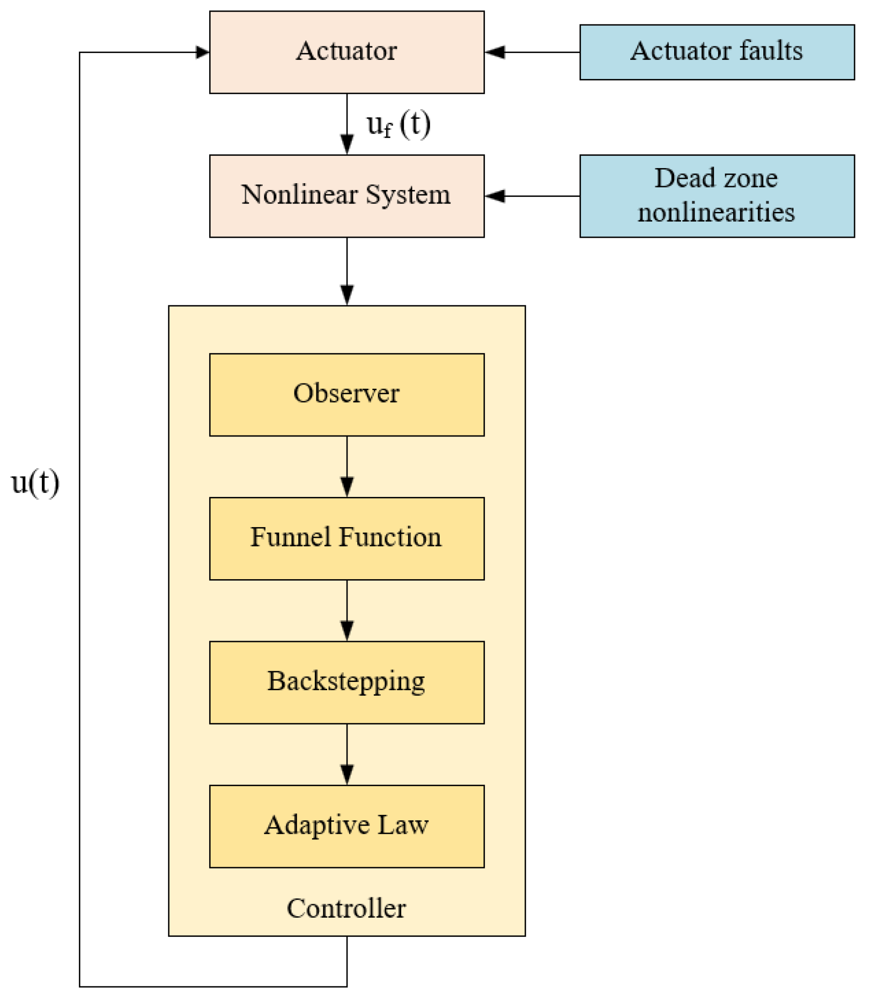
This section presents a novel fault-tolerant control strategy to overcome the challenges caused by actuator faults and unknown dead zones. The design procedure has three main stages: Construct a familiar state observer to estimate the unmeasurable states. Based on this, a prescribed-time funnel function is adopted to guarantee the specified transient performance requirements. Subsequently, an adaptive FTC scheme is formulated by combining a bound estimation approach with a backstepping procedure incorporating a Barrier Lyapunov function. The control strategy diagram is presented in Figure 2.

3.1. Adaptive State Observer Design

In system (1), the states x 1 , . . . , x n cannot be directly measured for feedback control. A state observer should be constructed to estimate the unmeasurable states to address this issue. Based on this observer, an adaptive output feedback strategy is proposed using the estimated states to compensate for system failures.
The observer model is designed as follows:
x ^ ˙ 1 = x ^ 2 + θ ^ T ϕ 1 ( x ^ 1 ) + L 1 ( y x ^ 1 ) , x ^ ˙ i = x ^ i + 1 + θ ^ T ϕ i ( x ^ i ) + L i ( y x ^ 1 ) , x ^ ˙ n = u + θ ^ T ϕ n ( x ^ n ) + L n ( y x ^ 1 ) ,
where i = 2 , , n 1 . The variables x ^ 1 , x ^ i , and x ^ n denote the estimates of x 1 , x i , and x n , respectively, while θ ^ 1 , θ ^ i , and θ ^ n denote the estimates of θ 1 , θ i , and θ n . The observer gains are denoted by L 1 , L i , and L n .
The observer error e 1 , e i , e n are constructed as follows:
e 1 = x 1 x ^ 1 , e i = x i x ^ i , e n = x n x ^ n ,
From (13) and (14), the following equation of observer error can be derived.
e ˙ = A e + F T ( x ^ i ) Θ ˜ + Δ F T Θ + d
where e = [ e 1 , . . . , e n ] T and F = d i a g { ϕ 1 ( x ^ 1 ) , . . . , ϕ n ( x ^ n ) } , Θ ˜ = Θ Θ ^ , G = d i a g { 1 , . . . , 1 } and Δ F = d i a g { ϕ 1 ( x 1 ) ϕ 1 ( x ^ 1 ) , . . . , ϕ n ( x n ) ϕ n ( x ^ n ) } and
A = L 1 L i G L n 0 , Θ ˜ = θ ˜ 1 θ ˜ i θ ˜ n , Θ = θ 1 θ i θ n , d = d 1 ( t ) d i ( t ) d n ( t )
There exists a common positive definite matrix P such that
A T P + P A < Q
where Q T = Q > 0 is given. The control gains L i are designed to guarantee the existence of a positive-definite solution P to the inequality
Choose a Lyapunov candidate function V 0 for (13) as:
V 0 = e T P e + 1 2 γ 0 Θ ˜ T Θ ˜
where γ 0 is a positive constant.
The time derivative of V 0 can be derived according to (15).
V ˙ 0 = e T Q e + 2 e T P [ F T ( x ^ 1 ) Θ ˜ + Δ F T Θ + d ] 1 γ 0 Θ ˜ T Θ ^ ˙
For the sake of employing the feedback information e 1 to construct the parameter adaptive laws, we partition the vector e as e = [ e 1 , 0 , , 0 ] + [ 0 , e 2 , , e n ] . By Young’s inequality and Assumptions 2–3, it follows that [see (10)–(13) given in Box 1], where e 10 = [ e 1 , 0 , , 0 ] T , I 1 = diag { 0 , 1 , , 1 } R n × n .
The following three inequalities can be derived based on Young’s inequality.
2 e T P F T ( x ^ i ) Θ ˜ 2 e 10 T P F T ( x ^ i ) Θ ˜ + e T I ¯ 1 P F T ( x ^ i ) F ( x ^ i ) P I ¯ 1 e + Θ ˜ T Θ ˜
2 e T P Δ F T Θ e T P P e + θ M 2 i = 1 n ( L i 2 e i 2 )
2 e T P d e T P P e + d M 2
Substituting ( 19 ) ( 21 ) into ( 15 ) yields that
V ˙ 0 e T Q ¯ e + Θ ˜ T Θ ˜ + d M 2 1 γ 0 Θ ˜ [ 2 γ 0 F ( x ^ i ) P e 10 Θ ^ ]
where Q ¯ is a additional auxiliary matrix.
Q ¯ = Q 2 P P m a x 1 i n ϕ i ( x ^ i ) I ¯ 1 P P I ¯ 1 θ M 2 i = 1 n ( L i 2 )
Design the adaptive updating law as follows
Θ ^ ˙ = 2 γ 0 F ( x ^ i ) P e 10 σ 0 Θ ^
where σ 0 is a positive constant.
By substituting ( 24 ) into ( 22 ) , the following time derivative of V 0 is obtained:
V ˙ 0 e T Q ¯ e ( σ 0 2 γ 0 1 ) Θ ˜ T Θ ˜ + d M 2 + σ 0 2 γ 0 Θ T Θ
From (25), we can obtain the stability of the observer error system in the sense of the Lyapunov function method by choosing the design parameter L = [ L 1 , , L n ] such that Q ˜ > 0 . However, Q is related to the variables x 1 , x ^ 2 , and it is seen that the existence of L cannot be ensured since the controlled system (10) may be unstable.

3.2. Adaptive Backstepping Controller Design

This subsection presents an adaptive control algorithm to guarantee that the tracking error e ( t ) is confined within a special funnel function while achieving asymptotic convergence. The algorithm’s control design employs the coordinate transformation.
z 1 = μ ( y y d )
z i = x ^ i α i 1 , ( i = 2 , 3 , . . . , n )
where the funnel function μ ( t ) is designed to satisfy Definition 1, y d is the desired output trajectory and α i 1 denotes the virtual control laws for iterative design.
  • Step 1: The dynamics of z 1 can be derived by combining (1) and the funnel function
z ˙ 1 = μ ˙ ( y y d ) + μ ( y ˙ y ˙ d ) = μ ˙ ( y y d ) + μ [ z 2 + α 1 + x ˜ 2 + θ 1 T ( t ) ϕ 1 ( x 1 ) + d 1 ( t ) y ˙ d ]
Construct the first valid candidate Lyapunov function V 1 as follows:
V 1 = 1 2 l o g 1 1 z 1 2 + 1 2 γ 11 ρ ˜ 1 T ρ ˜ 1 + 1 2 γ 12 D ˜ 1 2
where γ 11 > 0 , γ 12 > 0 , ρ ˜ 1 = θ 1 ρ ^ 1 is the parameter estimation error, and D ˜ 1 = D 1 D ^ 1 is the disturbance estimation error.
For | z 1 |   <   1 , the natural logarithm operator log(·) satisfies the condition that V 1 is positive definite and continuously differentiable. The time derivative of V 1 along ( 29 ) and Lemma 2 is obtained as follows:
V 1 ˙ = z 1 χ { μ ˙ ( y y d ) + μ [ z 2 + α 1 + x ˜ 2 + θ 1 T ( t ) ϕ 1 ( x 1 ) + d 1 ( t ) y ˙ d ] } 1 γ 11 ρ ˜ 1 ρ ^ ˙ 1 1 γ 12 D ˜ 1 D ^ ˙ 1 z 1 χ { μ ˙ ( y y d ) + μ [ z 2 + α 1 + x ˜ 2 + θ 1 T ( t ) ϕ 1 ( x 1 ) y ˙ d ] } + 0.2785 m D 1 + z 1 χ μ t a n h ( z 1 χ μ m ) D 1 1 γ 11 ρ ˜ 1 ρ ^ ˙ 1 1 γ 12 D ˜ 1 D ^ ˙ 1
where χ = 1 1 z 1 2 > 0 , which can be utilized in the controller design. Moreover, the second property of μ ( t ) guarantees the existence of a positive constant μ d M > 0 satisfying | μ ˙ ( t ) | μ d M .
The first virtual control input α 1 together with the update laws for ρ ^ 1 and D ^ 1 are defined as
α 1 = 1 μ χ ( c 1 z 1 ) μ ˙ μ ( y y d ) t a n h ( z 1 χ μ m ) D ^ 1 ρ ^ 1 T ϕ 1 ( x 1 ) + y ˙ d
ρ ^ ˙ 1 = γ 11 z 1 χ μ ϕ 1 ( x 1 ) σ 11 γ 11 ρ ^ 1
D ^ ˙ 1 = γ 12 z 1 χ μ t a n h ( z 1 χ μ m ) σ 12 γ 12 D ^ 1
where c 1 > 0 , σ 11 > 0 , σ 12 > 0 are positive constants.
The substitution of (31)–(33) into (30) yields, the time derivative of V 1 is obtained:
V 1 ˙ = c 1 z 1 2 + z 1 z 2 χ μ + z 1 χ μ x ˜ 2 + 0.2785 m D 1 + σ 11 ρ ˜ 1 ρ ^ 1 + σ 12 D ˜ 1 D ^ 1 ( c 1 1 2 ) z 1 2 + z 1 z 2 χ μ + 1 2 χ 2 μ 2 x ˜ 2 2 + 0.2785 m D 1 + ζ 11 σ 11 ρ 1 2 ( 1 1 ζ 11 ) σ 11 ρ ˜ 1 2 + ζ 12 σ 12 D 1 2 ( 1 1 ζ 12 ) σ 12 D ˜ 1 2
  • Step 2: The time derivative of z 2 can be derived by combining (13) and (27)
z ˙ 2 = x ^ ˙ 2 α ˙ 1 = z 3 + α 2 + L 2 x ˜ 1 + θ ^ 2 T ( t ) ϕ 2 ( x 2 ) α ˙ 1
Construct the second valid candidate Lyapunov function V 2 as follows:
V 2 = 1 2 z 2 2
From (31), the derivative of α 1 is obtained as:
α ˙ 1 = α 1 x 1 [ x ^ 2 + θ 1 T ( t ) ϕ 1 ( x 1 ) + x ˜ 2 + d 1 ( t ) ] + Δ 1
where Δ 1 = α 1 ρ ^ 1 ρ ^ ˙ 1 + k = 1 1 ( α 1 y d ( k ) ) y d ( k + 1 ) + k = 1 1 ( α 1 μ ( k ) ) μ ( k + 1 )
From (35)–(37), the derivative of V 2 is derived as
V ˙ 2 = z 2 [ z 3 + α 2 + L 2 x ˜ 1 + θ ^ 2 T ( t ) ϕ 2 ( x 2 ) α 1 x 1 x ˜ 2 α 1 x 1 θ 1 T ( t ) ϕ 1 ( x 1 ) α 1 x 1 d 1 ( t ) Δ 1 ]
By employing Young’s inequality, four terms in (38) can be bounded as follows:
z i L i x ˜ 1 1 2 L 2 2 z 2 2 + 1 2 x ˜ 1 2
z i α 1 x 1 x ˜ 2 1 2 z i 2 ( α 1 x 1 ) 2 + 1 2 x ˜ 2 2
z i α 1 x 1 θ 1 T ( t ) ϕ 1 ( x 1 ) 1 2 z i 2 ( α 1 x 1 ) 2 ϕ 1 T ( x 1 ) ϕ 1 ( x 1 ) + 1 2 θ M T θ M
z i α 1 x 1 d 1 ( t ) 1 2 z i 2 ( α 1 x 1 ) 2 + 1 2 D 1 2
Choose the second virtual control law α 2 as
α 2 = c 2 z 2 z 1 χ μ θ ^ 2 T ( t ) ϕ 2 ( x 2 ) + Δ 1 1 2 z 2 2 [ L 2 2 + 2 ( α 1 x 1 ) 2 + α 1 x 1 ϕ 1 T ( x 1 ) ϕ 1 ( x 1 ) ]
where c 2 is a positive constant.
By substituting of (39)–(43) into (38), we have
V ˙ 2 c 2 z 2 2 z 1 z 2 χ μ + z 2 z 3 + 1 2 x ˜ 1 2 + 1 2 x ˜ 2 2 + 1 2 θ M T θ M + D 1 2
  • Step i: The detailed derivation of step i is provided in Appendix A.
  • Step n: By combining (10) and (27), the derivative of z n can be obtained
z ˙ n = x ^ ˙ n α ˙ n 1 = u + L n x ˜ 1 + θ ^ n T ( t ) ϕ n ( x n ) α ˙ n 1
Because u ( t ) consists of gain faults and bias faults, according to (2)–(6), we obtain
u = B ψ v ( t ) + B τ + J = N v ( t ) + Ξ
where parameter N = B ψ and Ξ = B τ + J .
The derivative of α n 1 can be obtained
α ˙ n 1 = α n 1 x 1 [ x ^ 2 + θ 1 T ( t ) ϕ 1 ( x 1 ) + x ˜ 2 + d 1 ( t ) ] + Δ n 1
where Δ n 1 = α n 1 ρ ^ n 1 ρ ^ ˙ n 1 + k = 1 n 1 ( α n 1 y d ( k ) ) y d ( k + 1 ) + k = 1 n 1 ( α n 1 μ ( k ) ) μ ( k + 1 ) .
Construct the last valid candidate Lyapunov function V n as follows.
V n = 1 2 z n 2 + a 0 2 γ 2 ξ ˜ 2 + 1 2 γ 3 Ξ ˜ 2
where γ 2 > 0 , γ 3 > 0 . Since B is bounded such that 0 < B < 1 , the following definitions are introduced: a 0 = inf t 0 λ min ( N ) , and ξ = 1 a 0 .
By substituting (45)–(47) into the derivative of (48), V ˙ n can be obtained
V ˙ n = z n z ˙ n a 0 γ 2 ξ ˜ ξ ^ ˙ 1 γ 3 Ξ ˜ Ξ ^ ˙ = z n [ u + L n x ˜ 1 + θ ^ n T ( t ) ϕ n ( x n ) α ˙ n 1 ] a 0 γ 2 ξ ˜ ξ ^ ˙ 1 γ 3 Ξ ˜ Ξ ^ ˙ = z n [ N v ( t ) + Ξ + L n x ˜ 1 + θ ^ n T ( t ) ϕ n ( x n ) α n 1 x 1 x ˜ 2 α n 1 x 1 θ 1 T ( t ) ϕ 1 ( x 1 ) α n 1 x 1 d 1 ( t ) Δ n 1 ] a 0 γ 2 ξ ˜ ξ ^ ˙ 1 γ 3 Ξ ˜ Ξ ^ ˙ z n N v ( t ) + z n Ξ z n t a n h ( z n m ) Ξ + z n t a n h ( z n m ) Ξ + z n θ ^ n T ( t ) ϕ n ( x n ) z n Δ n 1 + 1 2 x ˜ 1 2 + 1 2 x ˜ 2 2 + 1 2 θ M T θ M + 1 2 z n 2 [ L 2 2 + 2 ( α n x 1 ) 2 + α n x 1 ϕ 1 T ( x 1 ) ϕ 1 ( x 1 ) + D 1 2 ] a 0 γ 2 ξ ˜ ξ ^ ˙ 1 γ 3 Ξ ˜ Ξ ^ ˙
Define an auxiliary variable β within as follows
β = c n z n + z n 1 Δ n 1 + θ ^ n T ( t ) ϕ n ( x n ) α n 1 x 1 θ ^ 1 T ( t ) ϕ 1 ( x 1 ) + t a n h ( z n m ) Ξ ^ 1 2 [ L n 2 + 2 ( α n x 1 ) 2 + α n x 1 ϕ 1 T ( x 1 ) ϕ 1 ( x 1 ) ]
where c n is a positive constant.
By incorporating the virtual variable β into (49), we derive
V ˙ n z n N v ( t ) + z n Ξ z n t a n h ( z n m ) Ξ + z n t a n h ( z n m ) Ξ z n t a n h ( z n m ) Ξ ^ c n z n 2 z n 1 z n + 1 2 x ˜ 1 2 + 1 2 x ˜ 2 2 + 1 2 θ M T θ M + 1 2 D 1 2 + z n β a 0 γ 2 ξ ˜ ξ ^ ˙ 1 γ 3 Ξ ˜ Ξ ^ ˙ z n N v ( t ) + 0.2785 m Ξ + z n t a n h ( z n m ) Ξ ˜ c n z n 2 z n 1 z n + 1 2 x ˜ 1 2 + 1 2 x ˜ 2 2 + 1 2 θ M T θ M + 1 2 D 1 2 + z n β a 0 γ 2 ξ ˜ ξ ^ ˙ 1 γ 3 Ξ ˜ Ξ ^ ˙
Invoking (47) and (51), we propose the following adaptive FTC strategy:
v ( t ) = z n ξ ^ 2 β 2 ξ ^ 2 z n 2 β 2 + η
where η > 0 .
According to Lemma 3 and (52), we obtain
z n N v ( t ) = N ξ ^ 2 z n 2 β 2 ξ ^ 2 z n 2 β 2 + η a 0 ξ ^ 2 z n 2 β 2 ξ ^ 2 z n 2 β 2 + η a 0 η a 0 ξ ^ z n β
And then the following time derivative of V n can be obtained:
V ˙ n a 0 η a 0 ξ ^ z n β + 0.2785 m Ξ + z n t a n h ( z n m ) Ξ ˜ c n z n 2 z n 1 z n + 1 2 x ˜ 1 2 + 1 2 x ˜ 2 2 + 1 2 θ M T θ M + z n β a 0 γ 2 ξ ˜ ξ ^ ˙ 1 γ 3 Ξ ˜ Ξ ^ ˙ a 0 η a 0 ξ z n β + z n β + 0.2785 m Ξ c n z n 2 z n 1 z n + 1 2 x ˜ 1 2 + 1 2 x ˜ 2 2 + 1 2 θ M T θ M + ξ ˜ [ a 0 z n β a 0 γ 2 ξ ^ ˙ ] + Ξ ˜ [ z n t a n h ( z n m ) 1 γ 3 Ξ ^ ˙ ]
Design the adaptive updating laws as follows
ξ ^ ˙ = γ 2 z n β γ 2 σ 2 ξ ^ Ξ ^ ˙ = γ 3 z n t a n h ( z n m ) γ 3 σ 3 Ξ ^
where σ 2 > 0 , σ 3 > 0 .
According to Lemma 1, two terms in (54) can be obtained.
a 0 σ 2 ξ ˜ ξ 1 ζ n 1 a 0 σ 2 ξ ˜ 2 + ζ n 1 a 0 σ 2 ξ 2
σ 3 Ξ ˜ Ξ 1 ζ n 2 σ 3 Ξ ˜ 2 + ζ n 2 σ 3 Ξ 2
where ζ n 1 > 0 and ζ n 2 > 0 are unknown constants. The substitution of (55)–(57) into ( 54 ) yields
V n ˙ a 0 η + 0.2785 m Ξ c n z n 2 z n 1 z n + 1 2 x ˜ 1 2 + 1 2 x ˜ 2 2 + 1 2 θ M T θ M + ζ n 1 a 0 σ 2 ξ 2 + ζ n 2 σ 3 Ξ 2 ( 1 1 ζ n 1 ) a 0 σ 2 ξ ˜ 2 ( 1 1 ζ n 2 ) σ 3 Ξ ˜ 2

3.3. Stability Analysis

The results of this study are summarized and formally given in Theorem 1.
Theorem 1.
Under Assumption 1, considering the parametric strict-feedback systems subject to actuator faults and symmetric dead-zone nonlinearities, together with the adaptive state observer (13), prescribed performance funnel (9), and adaptive virtual control (31), (43), (A4), adaptive updating laws (32)–(33) and (55), adaptive fault-tolerant controller (52), then there hold:
(1) 
It can be guaranteed that all closed-loop signals are globally bounded.
(2) 
The tracking error remains within the prescribed performance bounds imposed by the funnel function.
Proof. 
To analyze the stability of the proposed control strategy, a total Lyapunov function is constructed as follows:
V ˙ a l l = V 0 + V 1 + V 2 + . . . + V n e T ( Q ¯ n 1 2 I 1 n 1 2 I 2 ) e ( σ 0 2 γ 0 1 ) Θ ˜ T Θ ˜ + d M 2 + σ 0 2 γ 0 Θ T Θ + 1 2 χ 2 μ 2 x ˜ 2 2 + a 0 η + 0.2785 m D 1 + 0.2785 m Ξ ( c 1 1 2 ) z 1 2 i = 2 n c i z i 2 + n 1 2 θ M T θ M + ζ 11 σ 11 ρ 1 2 + ζ 12 σ 12 D 1 2 + ζ n 1 a 0 σ 2 ξ 2 + ζ n 2 σ 3 Ξ 2 ( 1 1 ζ 11 ) σ 11 ρ ˜ 1 2 ( 1 1 ζ 12 ) σ 12 D ˜ 1 2 ( 1 1 ζ n 1 ) a 0 σ 2 ξ ˜ 2 ( 1 1 ζ n 2 ) σ 3 Ξ ˜ 2 Λ V + ι
where I 1 = d i a g { 1 , 0 . . . 0 } , I 2 = d i a g { 0 , 1 . . . 0 } , Λ = m i n { λ m i n [ Q ¯ n 1 2 I 1 n 1 2 I 2 ] λ m i n , 2 γ 0 ( σ 0 2 γ 0 1 ) , 2 ( c 1 1 2 ) , 2 c 2 , . . . , 2 c n , 2 γ 11 σ 11 ( 1 1 ζ 11 ) , 2 γ 12 σ 12 ( 1 1 ζ 12 ) , 2 a 0 γ 2 σ 2 ( 1 1 ζ n 1 ) , 2 γ 3 σ 3 ( 1 1 ζ n 2 ) } , and ι = d M 2 + σ 0 2 γ 0 Θ T Θ + a 0 η + 0.2785 m D 1 + 0.2785 m Ξ + n 1 2 θ M T θ M + ζ 11 σ 11 ρ 1 2 + ζ 12 σ 12 D 1 2 + ζ n 1 a 0 σ 2 ξ 2 + ζ n 2 σ 3 Ξ 2 . □
To ensure the closed-loop stability, the parameters c 1 ,... c n , ζ 11 , ζ 12 , ζ n 1 , ζ n 2 should satisfy c 1 1 2 > 0 , c 2 > 0 c n > 0 , 1 1 ζ 11 > 0 , 1 1 ζ 12 > 0 , 1 1 ζ n 1 > 0 , 1 1 ζ n 2 > 0 , respectively.
To obtain the stability results, the observer design parameters L should be selected such that the LMI: A T P + P A 2 P P Ψ ( t ) I ¯ 1 P P I ¯ 1 + β 2 P B n B n T P θ M 2 i = 1 n ( L i 2 ) + n η 4 < 0 holds where m a x 1 i n ϕ i ( x ^ i ) .
Using Schur complement, the above inequality can be guaranteed by the following
( 1 , 1 ) * * * I ¯ 1 P Ψ 1 I * * P 0 I * β B n T P 0 0 I < 0
where ( 1 , 1 ) = A ¯ T P + P A ¯ + H T W + W H + ϕ I ¯ 1 , H = [ 1 0 0 0 ] , A ¯ = 0 G ^ 0 0 and G ^ G 1 , G 2 with G 1 = diag { 1 , 1 , , 1 } and G 2 = I n 1 . Moreover, L = P 1 W .
By integrating both sides of Equation (59), we obtain
e T P e e Λ t V ( 0 ) + ι Λ ( 1 e Λ t ) ,
which implies that
e ( t ) 1 λ m a x ( P ) ( e Λ t V ( 0 ) + ι Λ ( 1 e Λ t ) , t 0 ,
lim t e ( t ) 1 λ m a x ( P ) ι Λ .
It can be seen that the adverse effects caused by the actuator factor u f can be effectively compensated for. Additionally, the transient performance of the closed-loop system can be further improved by adjusting the design parameters γ 2 , σ 2 , γ 2 and σ 3 . The sensitivity selection of each parameter is summarized in Table 1.
Remark 6.
This study adopts a funnel function to prescribe the transient performance of the system, thereby achieving effective tracking. The distinctive feature of the proposed design lies in its ability to remove the initial-condition dependence commonly required in most PPB-based results, and to ensure a global prescribed transient performance regardless of initial states.
Remark 7.
In contrast to the methods in [12,13,14,15,16,17] and [20,21,22], which focus on systems with single types of constraints, this work addresses a more challenging multi-constraint problem involving actuator faults and unknown dead zones. By integrating output feedback, bound estimation, and adaptive techniques, the proposed control strategy achieves asymptotic tracking performance while significantly enhancing the robustness and adaptability of the system.
Remark 8.
From (59), it can be seen that the ultimate boundedness of the tracking error depends on the constants Λ and ι. To reduce the upper bound term 2 ι / Λ , either Λ can be increased or ι can be decreased. Based on the structure of (59), increasing Λ can be achieved by increasing c i , while decreasing ι can be achieved by increasing γ 1 , γ 2 , and γ 3 . However, it should be noted that Λ and ι are not independent; some design parameters (such as σ i ) affect both simultaneously, leading to a coupling relationship between them during the adjustment process. Therefore, relying solely on intuitive parameter adjustments is insufficient to effectively reduce 2 ι / Λ , which to some extent increases the complexity of performance optimization.
Remark 9.
From Equations (62) and (63), the observer error e i ( t ) converges exponentially with rate Λ / 2 in the disturbance-free case, and remains ultimately bounded in the presence of bounded disturbances, with the steady-state bound proportional to 2 ι / Λ . This demonstrates both the convergence rate and the robustness of the proposed observer.
Remark 10.
Table 2 shows that existing studies mainly focus on one of three issues—prescribed performance control, unknown dead zones, or actuator faults—while seldom addressing them in combination. A few works have considered two aspects simultaneously, but none of them tackle all three together. The proposed method fills this gap by integrating prescribed performance control, robustness against unknown dead zones, and fault-tolerant capability for actuator faults within a unified framework.

4. Simulation

To validate the effectiveness of the proposed control strategy, this paper conducts simulation studies on the dynamic response characteristics of a DC motor, systematically evaluating the control performance of this method under complex operating conditions. Therefore, it requires focused analysis. We consider the following DC motor model [35]
J y ¨ = k u D y ˙ F f + Δ ( t )
where the term J is the inertial load, the terms y, y ˙ , and y ¨ denote the motor’s angular displacement, angular velocity, and angular acceleration. Respectively. The parameter k represents the torque constant, the term u is the controller’s input, the term D is the viscous friction coefficient, the term F denotes the total friction torque, and the term Δ ( t ) represents other system disturbances.
To convert the motor inertial load dynamics (64) into state space equation form, we can express it as follows:
x ˙ 1 = x 2 x ˙ 2 = θ 1 u θ 2 x 2 θ 3 F f + Δ 1 ( t )
where θ 1 = k / J , θ 2 = D / J , θ 3 = 1 / J and Δ 1 ( t ) = Δ ( t ) / J . The term Δ 1 ( t ) denotes perturbations of the system, the term F f represents unmodeled errors which cause uncertainties. Assumption 1 is made because unmodeled dynamics in the system are always bounded.
Choose the following system parameters k = 0.3 , J = 1.0 , D = 2 . The external disturbance term F f adopts a nonlinear function form F f = tanh ( 700 x ( 0 ) ) to simulate complex disturbances in real-world conditions. To emulate actuator fault scenarios, a composite fault model is constructed: gain fault coefficient B = 0.8 + 0.1 s i n ( 0.5 t ) , bias fault as a spatiotemporal-varying function J ( t ) = 0.5 sin ( 1.5 t ) + 0.15 . The dead-zone parameters are set as b l = 0.2 , b r = 0.2 , and ψ = 1.2 . The desired trajectory is defined as y d = sin ( t ) . The funnel function μ ( t ) is defined by boundary parameter ρ = 0.2 , convergence precision ε = 0.05 , and adjustment time T s = 4 s .
Select the following initial conditions: x ^ 1 ( 0 ) = x ^ 2 ( 0 ) = 0.5 , θ ^ 1 ( 0 ) = [ 0.5 , 0.5 ] T , ζ ^ ( 0 ) = Ξ ^ ( 0 ) = 1 . The controller parameters are determined through multiple rounds of simulation tuning: c 1 = 25.50 , c 2 = 10 , γ 2 = 0.007 , γ 3 = 0.007 , σ 2 = 0.001 , σ 3 = 0.001 , η = 0.5 , and m = 0.5 . These parameters balance system response speed and control input smoothness. The observer gain L can be obtained as L = [ 15.84 80.57 ] T from (60). The evolutions of state observer are shown in Figure 3.
The dynamic responses of the considered motor are examined in seven cases as follows.
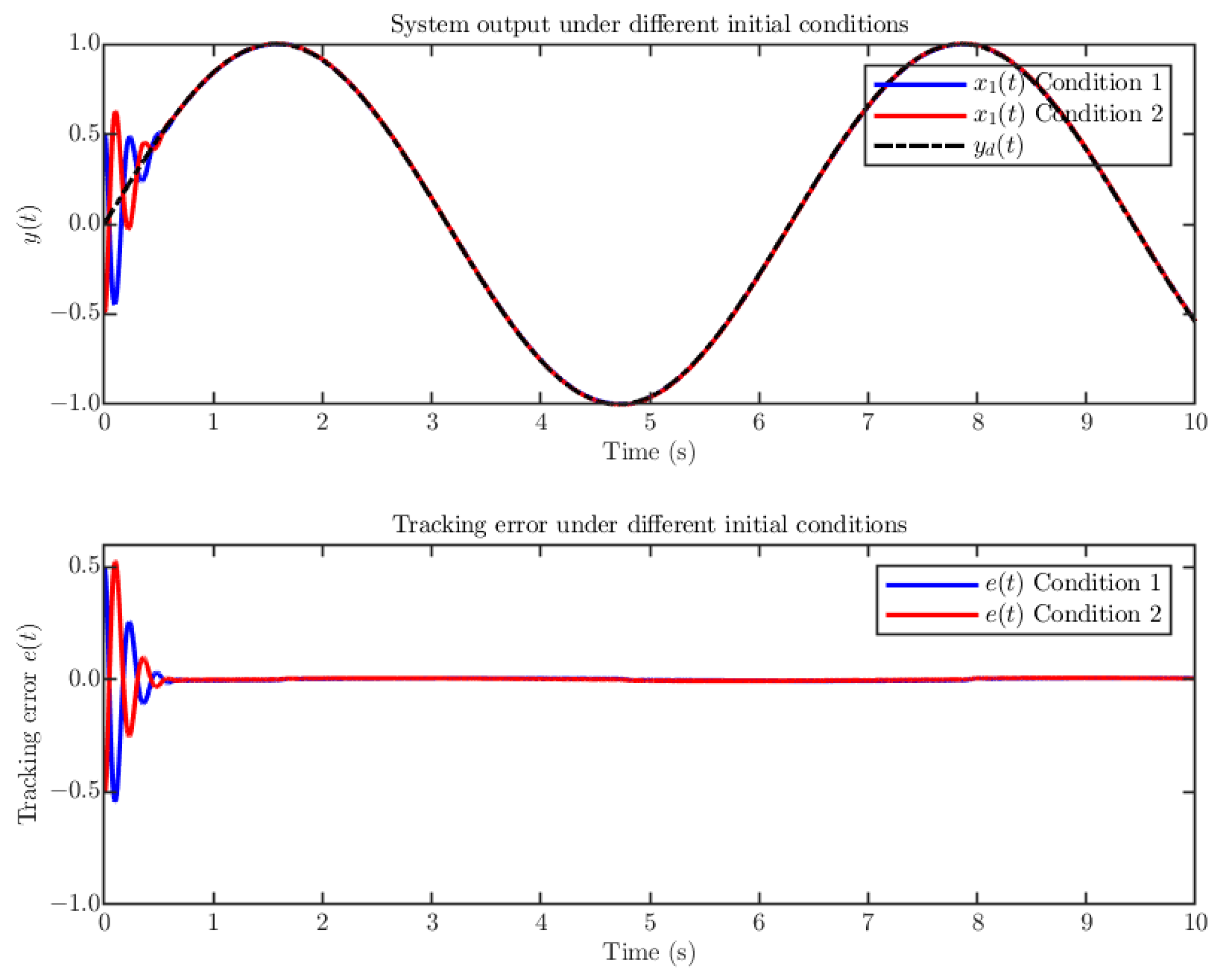
Case 1: Under two initial conditions: the considered motor is simulated under two initial conditions, i.e., ( x 1 ( 0 ) , x 2 ( 0 ) ) = ( 0.5 , 0.1 ) and ( 0.5 , 0.1 ) . The evolutions of y ( t ) and tracking error e ( t ) are displayed in Figure 4. It can be concluded from Figure 4 that, event under different initial conditions, tracking control can achieve convergence simultaneously.
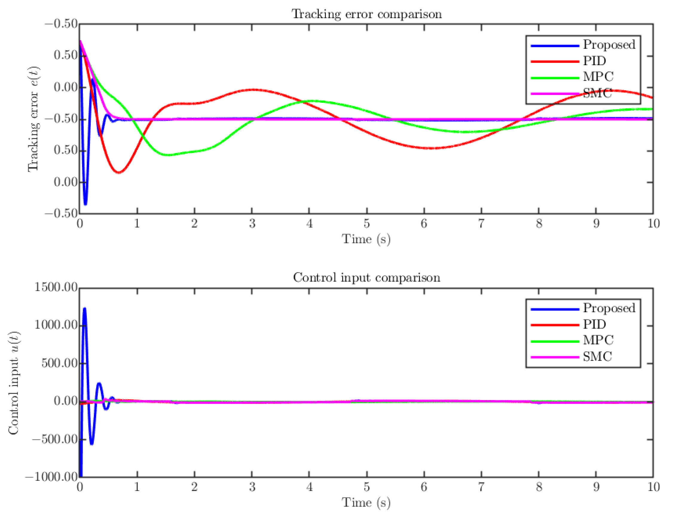
Case 2: To further illustrate the superiority of the proposed control method, the Nussbaum function method [36], PID control strategy, MPC method, and SMC method are adopted. The simulation results are shown in Figure 5. It can be concluded from Figure 5 that the tracking of the proposed control method converges faster and more stably, indicating that the proposed control method can achieve better convergence performance.
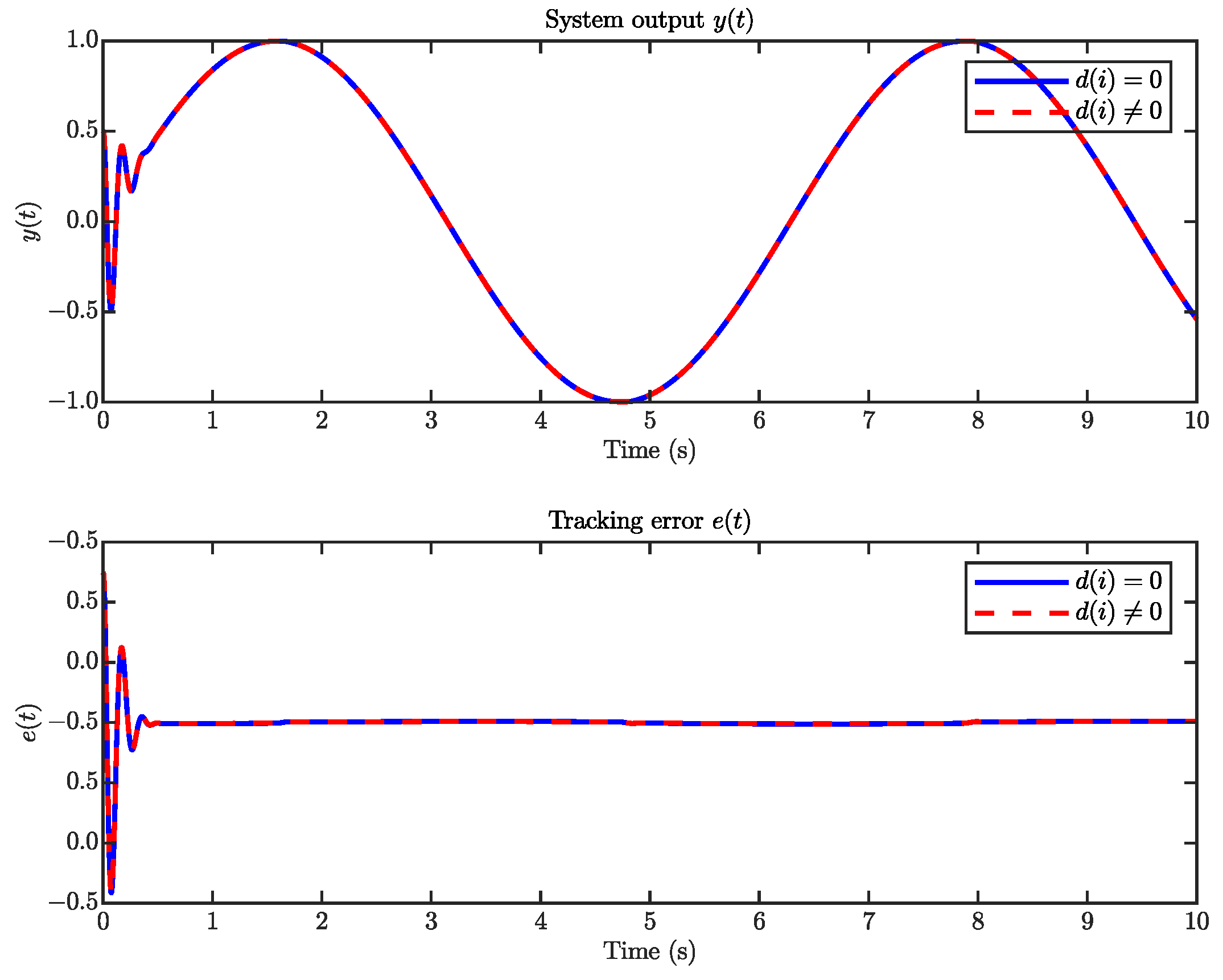
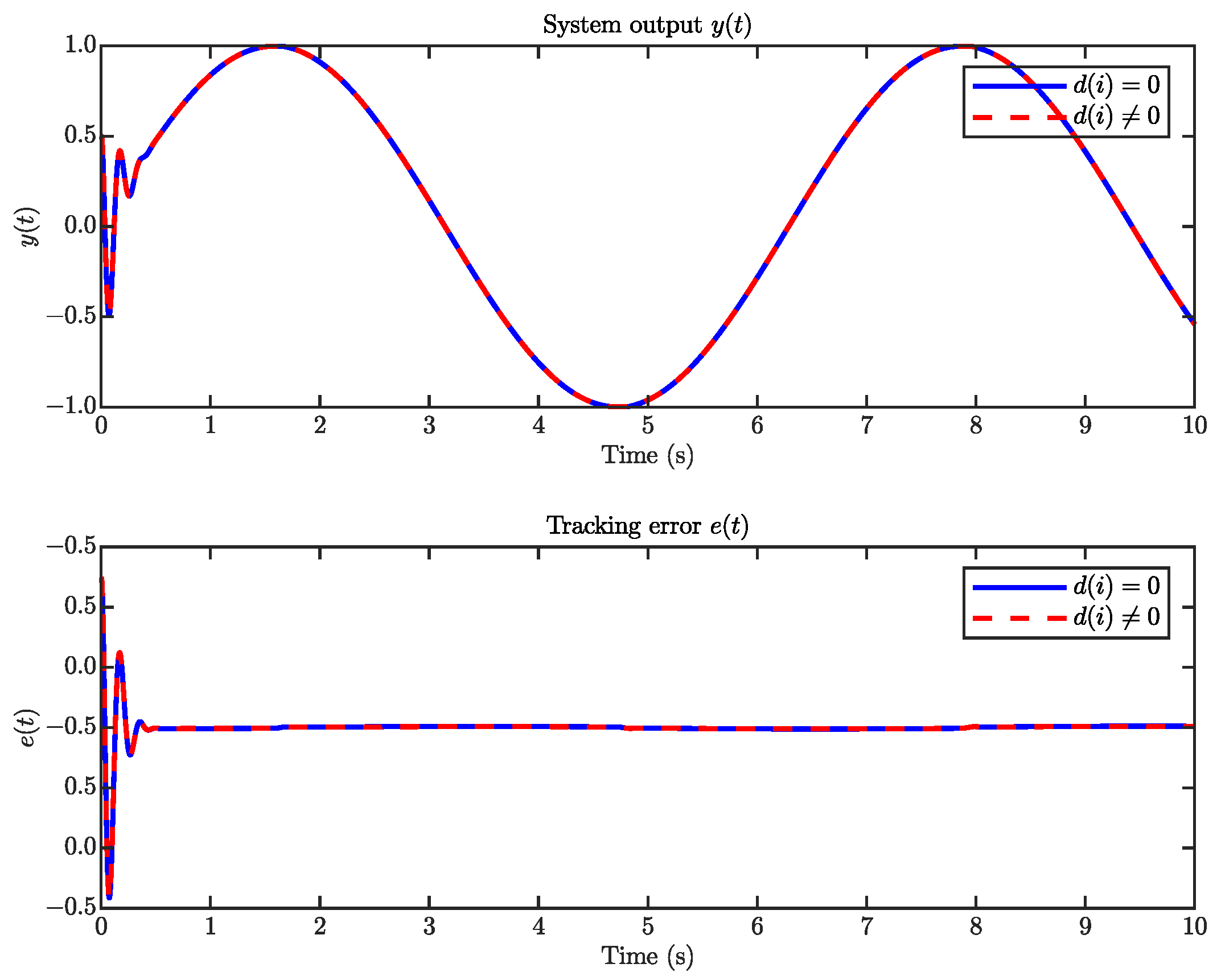
Case 3: Figure 6 illustrates the system output and tracking error under two conditions: without disturbance and with composite disturbance. The composite disturbance includes periodic pulses with an amplitude of 2 every 2 s, a sinusoidal disturbance 0.02 cos ( t ) , and zero-mean Gaussian white noise N ( 0 , 0 . 02 2 ) . A composite actuator fault occurs at t = 3 s in both scenarios. The results show that the system operates well under disturbances, with the tracking error exhibiting only slight fluctuations and remaining within 5 × 10 3 .
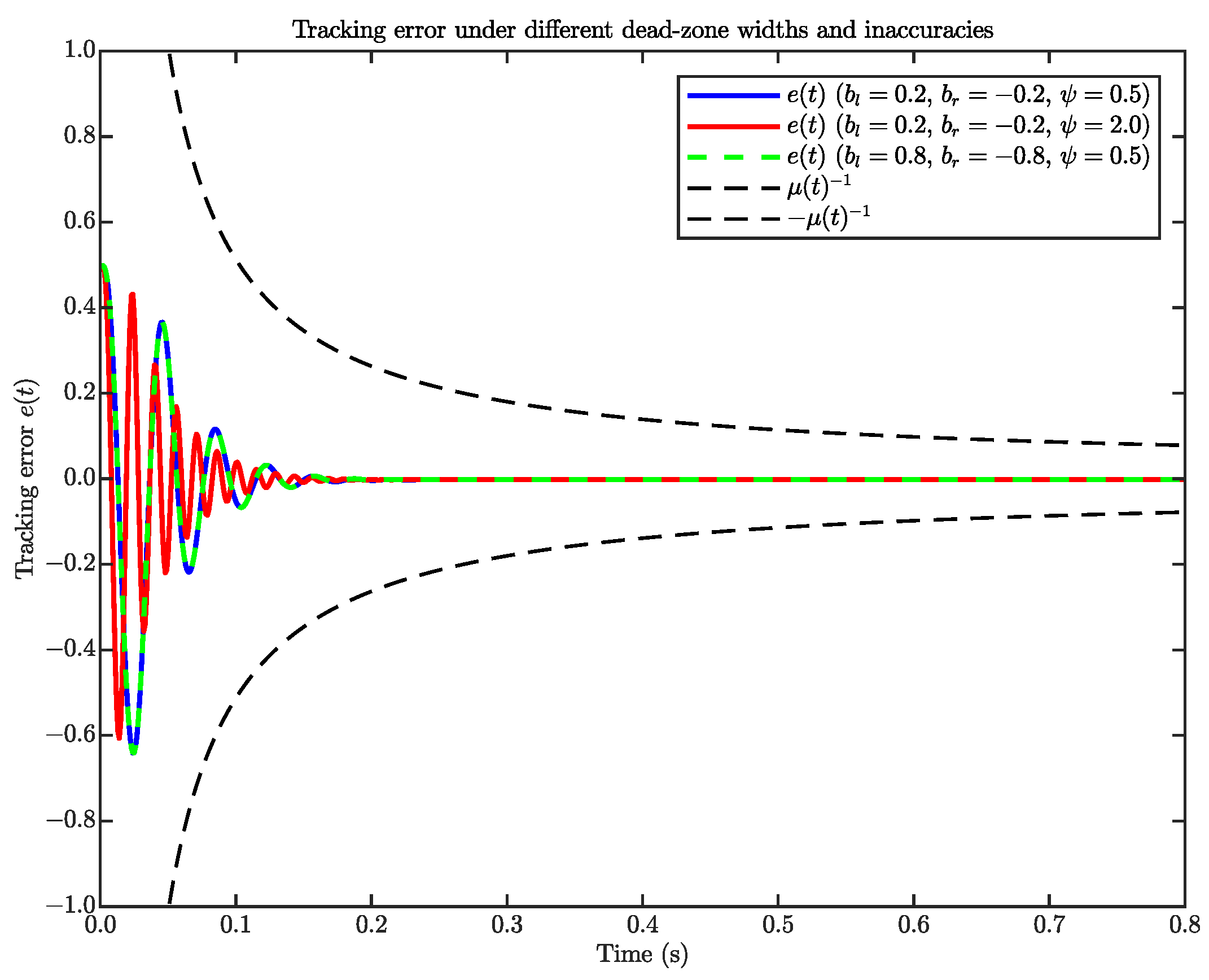
Case 4: Under different dead-zone widths and inaccuracies: Figure 7 analyzes the impact of dead-zone parameters on tracking error, which demonstrates the proposed controller’s robustness to dead-zone variations via adaptive nonlinear compensation, validating its applicability in scenarios with actuator nonlinearity fluctuations.
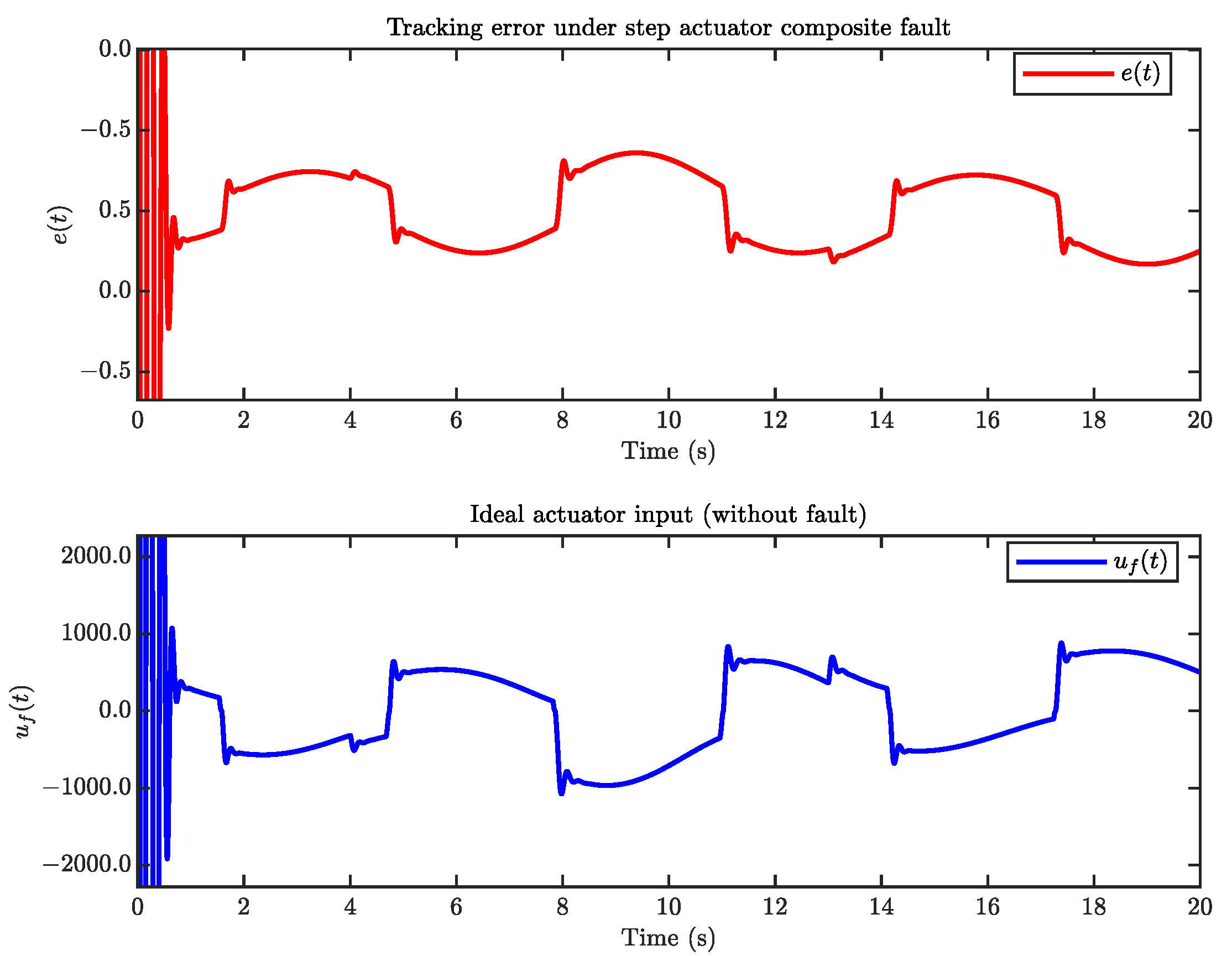
Case 5: Under the influence of different step-bias faults: Figure 8 aims to verify that the system maintains good operational performance under the influence of different step-bias faults with J ( t ) = 0.5 sin ( 1.5 t ) + 2 H ( t t 1 ) 4 H ( t t 2 ) , t 1 = 4 , t 2 = 13 where H ( · ) denotes the unit step function. At t = 4 s, the bias undergoes a positive step change (+2), and at t = 13 s it undergoes a negative step change ( 4 ), thereby constructing a composite bias fault with distinct abrupt transition characteristics. Figure 8 demonstrates that under the aforementioned offset fault, the proposed control strategy still ensures that the tracking error e ( t ) remains bounded. Overall results demonstrate that the designed controller significantly reduces tracking error under various step-bias conditions while ensuring stable system operation.
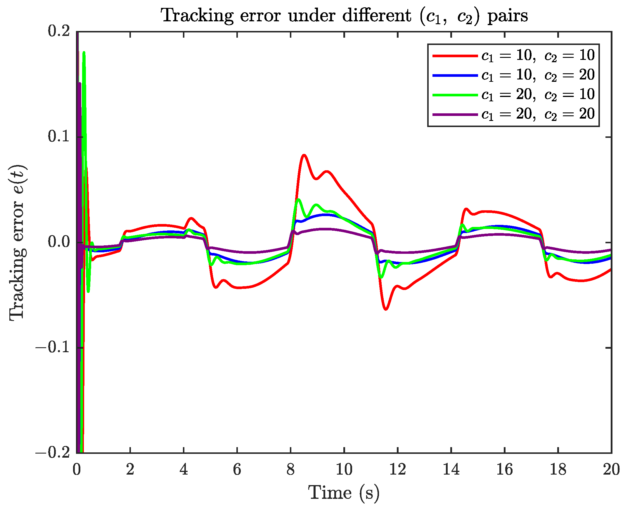
Case 6: Under different controller parameters: Figure 9 investigates the influence of key controller parameters ( c 1 and c 2 ) on tracking error. Results show that within the tested ranges ( c 1 [ 10 , 20 ] , c 2 [ 10 , 20 ] ), increasing c 1 significantly accelerates error convergence (reduced settling time) and improves transient smoothness (40% lower oscillation amplitude), while higher c 2 enhances disturbance rejection, reducing error fluctuations from 0.08 to 0.03.
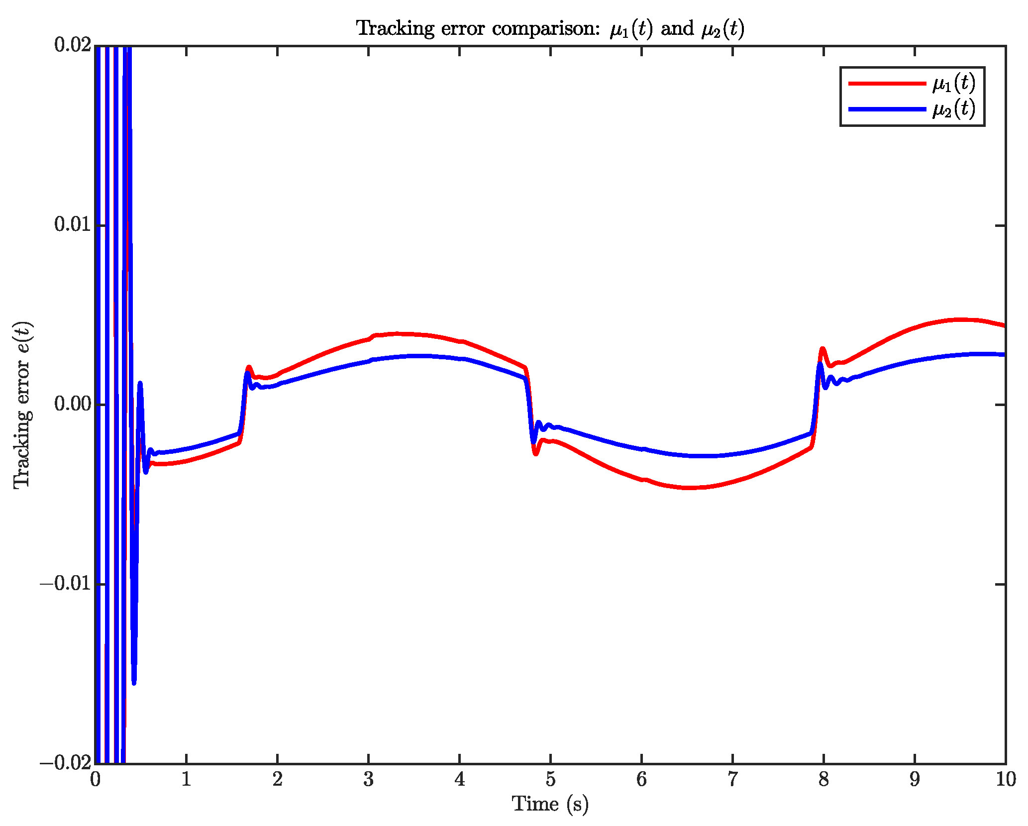
Case 7: Under different funnel functions: Figure 10 presents the performance of the tracking error under different funnel functions ( μ 1 ( t ) and μ 2 ( t ) ), where μ 1 ( t ) and μ 2 ( t ) denote the funnel functions. The parameters of μ 1 ( t ) are set as p = 2 , ε = 0.05 , T s = 4 s and μ 2 ( t ) is parameterized by ρ = 0.4 , ε = 0.05 , T s = 4 s. The comparison shows that the tracking error curves under the two funnel functions are nearly overlapping, indicating similar dynamic performance. Both tracking errors converge within 1s and remain strictly bounded, which confirms that the choice of different funnel functions does not significantly affect the tracking performance or control effort.

5. Conclusions

This paper investigates the adaptive fault-tolerant control problem for nonlinear high-order systems subject to actuator faults and dead-zone nonlinearities. Based on the funnel function, Barrier Lyapunov function method, and adaptive technique, a novel prescribed-time performance adaptive fault-tolerant control is proposed, which guarantees prescribed transient performance control with a convergence time of 0.8 s and a steady-state tracking error within ± 0.05 , independent of initial conditions. Theoretical analysis confirms global stability, and simulation results demonstrate superior robustness and tracking accuracy compared with conventional methods. In future work, we will continue investigating saturation control and higher-order motor systems and further explore applying theoretical findings to experimental work.

Author Contributions

Conceptualization, S.X. and S.H.; methodology, S.H.; software, Z.W.; validation, T.K. and P.N.; formal analysis, Z.W.; investigation, S.X.; resources, Z.W.; data curation, T.K. and N.K.; writing—original draft preparation, Z.W.; writing—review and editing, S.H.; visualization, S.X.; supervision, S.H.; project administration, S.X.; funding acquisition, Z.W. All authors have read and agreed to the published version of the manuscript.

Funding

This research received no external funding.

Data Availability Statement

Data are contained within the article.

Conflicts of Interest

The authors declare no conflicts of interest.

Appendix A

  • Step i ( i 2 ): The dynamics of z i can be derived by combining (10) and (27)
z ˙ i = x ^ ˙ i α ˙ i 1 = x ^ i + 1 + L i x ˜ 1 + θ ^ i T ( t ) ϕ i ( x i ) α ˙ i 1 = z i + 1 + α i + L i x ˜ 1 + θ ^ i T ( t ) ϕ i ( x i ) α ˙ i 1
The following valid candidate Lyapunov function V i + 1 is constructed
V i = 1 2 z i 2
The derivative of α i 1 can be calculated
α ˙ i 1 = α i 1 x 1 [ x ^ 2 + θ 1 T ( t ) ϕ 1 ( x 1 ) + x ˜ 2 + d 1 ( t ) ] + Δ i 2
The following virtual control law α i + 1 is chosen as
α i = c i z i z i 1 θ ^ i T ( t ) ϕ i ( x i ) + Δ i 1 1 2 z i 2 [ L i 2 + 2 ( α i x 1 ) 2 + α i 1 x 1 ϕ 1 T ( x 1 ) ϕ 1 ( x 1 ) ]
where c i is a positive constant.
By substituting Equations (A3) and (A4), the derivative of V ˙ i + 1 can be obtained
V ˙ i = z i [ z i + 1 + α i + L i x ˜ 1 + θ ^ i T ( t ) ϕ i ( x i ) α i 1 x 1 x ˜ 2 α i 1 x 1 θ 1 T ( t ) ϕ 1 ( x 1 ) α i 1 x 1 d 1 ( t ) Δ i 1 ] c i z i 2 + z i z i + 1 z i 1 z i + 1 2 x ˜ 1 2 + 1 2 x ˜ 2 2 + 1 2 θ M T θ M + D 1 2 .

References

  1. Liu, Y.; Wang, Y.; Guan, X.; Hu, T.; Zhang, Z.; Jin, S.; Wang, Y.; Hao, J.; Li, G. Direction and Trajectory Tracking Control for Nonholonomic Spherical Robot by Combining Sliding Mode Controller and Model Prediction Controller. IEEE Robot. Autom. Lett. 2022, 7, 11617–11624. [Google Scholar] [CrossRef]
  2. Huo, J.; Ji, H.; Yang, P. Research on Sensorless Control System of Permanent Magnet Synchronous Motor for CNC Machine Tool. In Proceedings of the 2021 40th Chinese Control Conference (CCC), Shanghai, China, 26–28 July 2021; pp. 1592–1595. [Google Scholar]
  3. Fan, L.; Zhu, Q.; Zheng, W.X. Stability Analysis of Switched Stochastic Nonlinear Systems with State-Dependent Delay. IEEE Trans. Autom. Control 2024, 69, 2567–2574. [Google Scholar] [CrossRef]
  4. Zhu, Q. Event-Triggered Sampling Problem for Exponential Stability of Stochastic Nonlinear Delay Systems Driven by Lévy Processes. IEEE Trans. Autom. Control 2025, 70, 1176–1183. [Google Scholar] [CrossRef]
  5. Sain, C.; Biswas, P.K.; Satpathy, P.R.; Babu, T.S.; Alhelou, H.H. Self-Controlled PMSM Drive Employed in Light Electric Vehicle—Dynamic Strategy and Performance Optimization. IEEE Access 2021, 9, 57967–57975. [Google Scholar] [CrossRef]
  6. Zhang, J.; Ren, W.; Sun, X.M. Current-Constrained Adaptive Robust Control for Uncertain PMSM Drive Systems: Theory and Experimentation. IEEE Trans. Transp. Electrif. 2023, 9, 4158–4169. [Google Scholar] [CrossRef]
  7. El-Sousy, F.F.M.; Alenizi, F.A.F. Optimal Adaptive Super-Twisting Sliding-Mode Control Using Online Actor-Critic Neural Networks for Permanent-Magnet Synchronous Motor Drives. IEEE Access 2021, 9, 82508–82534. [Google Scholar] [CrossRef]
  8. Zhao, Z.; Ren, Y.; Mu, C.; Zou, T.; Hong, K.S. Adaptive Neural-Network-Based Fault-Tolerant Control for a Flexible String with Composite Disturbance Observer and Input Constraints. IEEE Trans. Cybern. 2022, 52, 12843–12853. [Google Scholar] [CrossRef]
  9. Zhao, Z.; Liu, Z.; He, W.; Hong, K.S.; Li, H.X. Boundary Adaptive Fault-Tolerant Control for a Flexible Timoshenko Arm with Backlash-Like Hysteresis. Automatica 2021, 130, 109690. [Google Scholar] [CrossRef]
  10. Khalili, M.; Zhang, X.; Cao, Y.; Polycarpou, M.M.; Parisini, T. Distributed Fault-Tolerant Control of Multiagent Systems: An Adaptive Learning Approach. IEEE Trans. Neural Netw. Learn. Syst. 2020, 31, 420–432. [Google Scholar] [CrossRef]
  11. Gong, J.; Yu, X.; Pan, H.; Rodríguez-Andina, J.J. Adaptive Fault-Tolerant Control of Linear Motors Under Sensor and Actuator Faults. IEEE Trans. Transp. Electrif. 2024, 10, 9829–9838. [Google Scholar] [CrossRef]
  12. Guo, B.; Chen, Y. Robust Adaptive Fault-Tolerant Control of Four-Wheel Independently Actuated Electric Vehicles. IEEE Trans. Ind. Inform. 2020, 16, 2882–2894. [Google Scholar] [CrossRef]
  13. Wang, X.; Pan, L.; Tian, Y.; Liu, Y.; Li, L. Adaptive Fault-Tolerant Fixed-Time Sliding Mode Tracking Control for Steer-by-Wire System with Dual-Three-Phase PMSM. IEEE Trans. Veh. Technol. 2025, 74, 7554–7564. [Google Scholar] [CrossRef]
  14. Wang, D.; Gu, T.; Zhang, K. Fault Tolerant Control of 4-Wheel Independent Drive Vehicle Subject to Actuator Faults Based on Feasible Region. IEEE Trans. Veh. Technol. 2024, 73, 1652–1666. [Google Scholar] [CrossRef]
  15. Wang, J.; Zheng, Y.; Ding, J.; Zhang, H.; Sun, J. Memory-Based Event-Triggered Fault-Tolerant Consensus Control of Nonlinear Multi-Agent Systems and Its Applications. IEEE Trans. Autom. Sci. Eng. 2025, 22, 7941–7954. [Google Scholar] [CrossRef]
  16. Shi, H.; Gao, W.; Jiang, X.; Su, C.; Li, P. Two-dimensional model-free Q-learning-based output feedback fault-tolerant control for batch processes. Comput. Chem. Eng. 2024, 182, 108583. [Google Scholar] [CrossRef]
  17. Wu, C.; Liu, J.; Xiong, Y.; Wu, L. Observer-Based Adaptive Fault-Tolerant Tracking Control of Nonlinear Nonstrict-Feedback Systems. IEEE Trans. Neural Netw. Learn. Syst. 2018, 29, 3022–3033. [Google Scholar] [CrossRef]
  18. Astolfi, D.; Alessandri, A.; Zaccarian, L. Stubborn and Dead-Zone Redesign for Nonlinear Observers and Filters. IEEE Trans. Autom. Control 2021, 66, 667–682. [Google Scholar] [CrossRef]
  19. Casadei, G.; Astolfi, D.; Alessandri, A.; Zaccarian, L. Synchronization in Networks of Identical Nonlinear Systems via Dynamic Dead Zones. IEEE Control. Syst. Lett. 2019, 3, 667–672. [Google Scholar] [CrossRef]
  20. Li, D.Y.; Li, P.; Cai, W.C.; Song, Y.D.; Chen, H.J. Adaptive Fault-Tolerant Control of Wind Turbines with Guaranteed Transient Performance Considering Active Power Control of Wind Farms. IEEE Trans. Ind. Electron. 2018, 65, 3275–3285. [Google Scholar] [CrossRef]
  21. Jiang, B.; Hu, Q.; Friswell, M.I. Fixed-Time Attitude Control for Rigid Spacecraft with Actuator Saturation and Faults. IEEE Trans. Control. Syst. Technol. 2016, 24, 1892–1898. [Google Scholar] [CrossRef]
  22. Ding, L.; Li, S.; Gao, H.; Liu, Y.J.; Huang, L.; Deng, Z. Adaptive Neural Network-Based Finite-Time Online Optimal Tracking Control of the Nonlinear System with Dead Zone. IEEE Trans. Cybern. 2021, 51, 382–392. [Google Scholar] [CrossRef]
  23. Ma, Z.; Ma, H. Improved Adaptive Fuzzy Output-Feedback Dynamic Surface Control of Nonlinear Systems with Unknown Dead-Zone Output. IEEE Trans. Fuzzy Syst. 2021, 29, 2122–2131. [Google Scholar] [CrossRef]
  24. Bechlioulis, C.P.; Rovithakis, G.A. Robust Adaptive Control of Feedback Linearizable MIMO Nonlinear Systems with Prescribed Performance. IEEE Trans. Autom. Control 2008, 53, 2090–2099. [Google Scholar] [CrossRef]
  25. Ilchmann, A.; Ryan, E.P.; Sangwin, C.J. Tracking with Prescribed Transient Behaviour. ESAIM: Control. Optim. Calc. Var. 2002, 7, 471–493. [Google Scholar] [CrossRef]
  26. Ilchmann, A.; Ryan, E.P.; Trenn, S. Tracking Control: Performance Funnels and Prescribed Transient Behaviour. Syst. Control. Lett. 2005, 54, 655–670. [Google Scholar] [CrossRef]
  27. Theodorakopoulos, A.; Rovithakis, G.A. A Simplified Adaptive Neural Network Prescribed Performance Controller for Uncertain MIMO Feedback Linearizable Systems. IEEE Trans. Neural Netw. Learn. Syst. 2015, 26, 589–600. [Google Scholar] [CrossRef] [PubMed]
  28. Bechlioulis, C.P.; Rovithakis, G.A. Adaptive Control with Guaranteed Transient and Steady State Tracking Error Bounds for Strict Feedback Systems. Automatica 2009, 45, 532–538. [Google Scholar] [CrossRef]
  29. Xu, W.D.; Guo, X.G.; Li, Q.; Wang, J.L.; Park, J.H. PTNDO-based distributed active fault-tolerant control for leader–follower vehicular formation with unknown direction faults. Automatica 2025, 182, 112540. [Google Scholar] [CrossRef]
  30. Berger, T.; Lê, H.H.; Reis, T. Funnel Control for Nonlinear Systems with Known Strict Relative Degree. Automatica 2018, 87, 345–357. [Google Scholar] [CrossRef]
  31. He, Z.; Hu, J.; Wang, Y.; Cong, J.; Bian, Y.; Han, L. Attitude-Tracking Control for Over-Actuated Tailless UAVs at Cruise Using Adaptive Dynamic Programming. Drones 2023, 7, 294. [Google Scholar] [CrossRef]
  32. Berger, T. Fault-Tolerant Funnel Control for Uncertain Linear Systems. IEEE Trans. Autom. Control 2021, 66, 4349–4356. [Google Scholar] [CrossRef]
  33. Berger, T.; Ilchmann, A.; Ryan, E.P. Funnel Control of Nonlinear Systems. Math. Control. Signals Syst. 2021, 33, 151–194. [Google Scholar] [CrossRef]
  34. Verginis, C.K.; Dimarogonas, D.V. Asymptotic Tracking of Second-Order Nonsmooth Feedback Stabilizable Unknown Systems with Prescribed Transient Response. IEEE Trans. Autom. Control 2021, 66, 3296–3302. [Google Scholar] [CrossRef]
  35. Xu, Z.; Sun, C.; Liu, Q. Output-feedback prescribed performance control for the full-state constrained nonlinear systems and its application to DC motor system. IEEE Trans. Syst. Man Cybern. Syst. 2023, 53, 3898–3907. [Google Scholar] [CrossRef]
  36. Yao, D.; Xie, X.; Ahn, C.K. Adaptive fuzzy predefined accuracy control for output feedback cooperation of nonlinear multiagent systems under input quantization. IEEE Trans. Fuzzy Syst. 2023, 32, 2283–2296. [Google Scholar] [CrossRef]
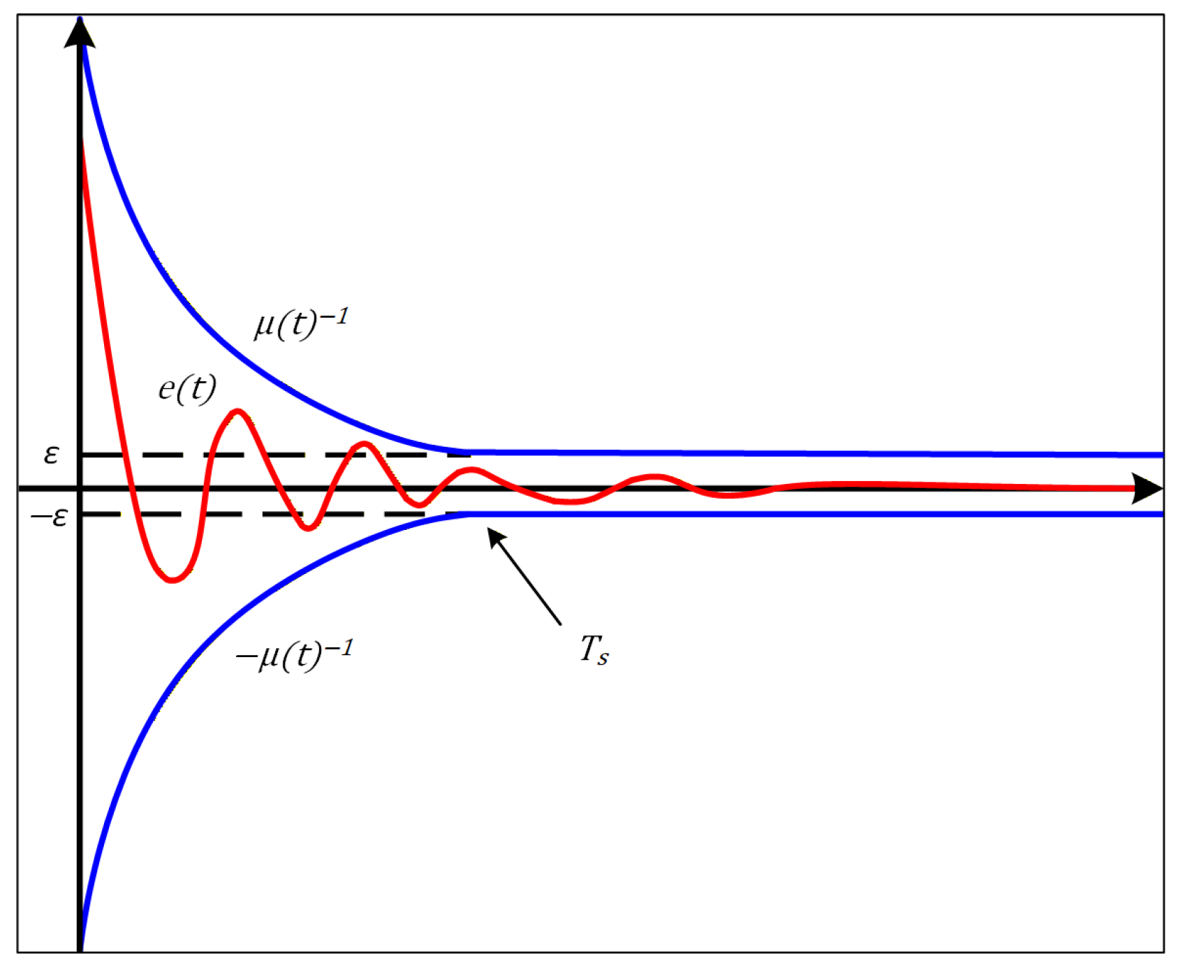
Figure 1. Evolution of the Tracking Error.
Symmetry 17 01915 g001
Figure 2. Control strategy diagram.
Symmetry 17 01915 g002
Figure 3. Evolutions of state x 1 , x 2 and state observer x ^ 1 , x ^ 2 .
Symmetry 17 01915 g003
Figure 4. System output and tracking error under different initial conditions.
Symmetry 17 01915 g004
Figure 5. Performance comparison between the proposed control and Nussbaum function method [36], PID method, MPC method, and SMC method.
Symmetry 17 01915 g005
Figure 6. System output x 1 and tracking error under no disturbances and composite disturbances.
Symmetry 17 01915 g006
Figure 7. Tracking error under different dead-zone widths and inaccuracies.
Symmetry 17 01915 g007
Figure 8. System output and tracking error under different step-bias faults.
Symmetry 17 01915 g008
Figure 9. Tracking error e ( t ) under different design parameters.
Symmetry 17 01915 g009
Figure 10. Tracking error under different funnel functions.
Symmetry 17 01915 g010
Table 1. Simulation Parameters.
ParametersValueParameterValue
γ 0 γ 0 > 0 γ 11 γ 11 > 0
σ 0 σ 0 > 0 σ 11 σ 11 > 0
L 1 L 1 > 0 γ 12 γ 12 > 0
L 2 L 2 > 0 σ 12 σ 12 > 0
mm > 0 γ 2 γ 2 > 0
η η > 0 σ 2 σ 2 > 0
ζ 11 0 < ζ 11 < 1 γ 3 γ 3 > 0
ζ 12 0 < ζ 12 < 1 σ 3 σ 3 > 0
ζ n 1 0 < ζ n 1 < 1 c 1 c 1 > 0.5
ζ n 2 0 < ζ n 2 < 1 c 2 c 2 > 0
ε 0 < ε < 1 c 3 c 3 > 0
T s T s > 1
ρ 0 < ρ < 1
Table 2. Comparison and Classifications of Some Studies.
Item of Comparison[6,7,8,9,10,11,12,13][14,15][16,17,18,19,20,21][22,23,24,25,26,27,28][29][30]This Paper
Prescribed performance control×××
Unknown dead zones×××
Actuator faults×××
Note: “✓” denotes that the corresponding reference addresses the related research aspect, whereas “×” denotes that it does not.
Disclaimer/Publisher’s Note: The statements, opinions and data contained in all publications are solely those of the individual author(s) and contributor(s) and not of MDPI and/or the editor(s). MDPI and/or the editor(s) disclaim responsibility for any injury to people or property resulting from any ideas, methods, instructions or products referred to in the content.