Abstract
Deep-sea submersibles, often featuring a symmetrical design for hydrodynamic stability, operate as safety-critical systems in extreme environments, where the tight dynamic coupling between subsystems like hydraulics and propulsion creates complex failure modes that are challenging to diagnose. A localized fault in one system can propagate, inducing anomalous behavior in another and confounding conventional single-system monitoring approaches. This paper introduces a novel unsupervised anomaly detection framework, the Dual-Stream Coupled Autoencoder (DSC-AE), designed specifically to address this cross-system fault challenge. Our approach leverages a dual-encoder, single-decoder architecture that explicitly models the normal coupling relationship between the hydraulic and propulsion systems by forcing them into a shared latent representation. This architectural design establishes a holistic and accurate baseline of healthy, system-wide operation. Any deviation from this learned coupling manifold is robustly identified as an anomaly. We validate our model using real-world operational data from the deep-sea submersible, including curated test cases of intra-system and inter-system faults. Furthermore, we demonstrate that the proposed framework offers crucial diagnostic interpretability; by analyzing the model’s reconstruction error heatmaps, it is possible to trace fault origins and their subsequent propagation pathways, providing intuitive and actionable decision support for submersible operation and maintenance. This powerful diagnostic capability is substantiated by superior quantitative performance, where the DSC-AE significantly outperforms baseline methods in detecting propagated faults, achieving higher accuracy and recall, among other performance metrics.
1. Introduction
Deep-sea submersibles are indispensable platforms for deep-ocean resource exploration, environmental monitoring, and scientific discovery. Their sustained and reliable operation is critical for the execution of national maritime strategies and the success of ambitious research missions. Operating in extreme underwater environments, these vehicles are subjected to immense hydrostatic pressure, low temperatures, corrosive conditions, and unpredictable terrain, which collectively impose stringent reliability requirements on all critical subsystems, including hydraulics, propulsion, power, and control. The failure of a single subsystem can trigger cascading failures across the vehicle, leading to mission abortion or, in the worst case, catastrophic safety incidents. Consequently, the development of intelligent anomaly detection systems for deep-sea submersibles is of paramount engineering and practical significance, directly enhancing their operational safety and mission success rates. This challenge of ensuring reliability in tightly coupled, safety-critical systems is not unique to underwater vehicles; it is a fundamental problem in many modern technological domains, including the management of large-scale Internet of Things (IoT) fleets and the security of software-defined networks (SDN).
The hydraulic and propulsion systems of a deep-sea submersible are characterized by tight physical coupling and intricate dynamic interactions. The hydraulic system actuates mission-critical tools such as manipulator arms and sampling devices, requiring dynamic adjustments of pressure and flow. Concurrently, the propulsion system, typically comprising multiple thrusters in a symmetrical arrangement to ensure balanced control, provides the necessary forces for navigation, station-keeping, and attitude stabilization. During normal operations, these two systems function in a coordinated manner under a supervisory control system. For instance, the abrupt extension of a manipulator arm alters the submersible’s center of gravity, necessitating an immediate compensatory response from the propulsion system to maintain stability. While such strong, synergistic coupling is fundamental to executing complex tasks, it also creates pathways for fault propagation. A local fault originating in one subsystem, such as diminished efficiency in a thruster, can induce anomalous operating conditions in the other, like abnormal pressure fluctuations in the hydraulic system as it attempts to compensate for the thrust imbalance. Conventional diagnostic models, typically designed for isolated subsystems, struggle to disambiguate between these benign synergistic operations and veritable fault propagation, rendering them susceptible to high rates of false alarms or missed detections. Furthermore, formulating an accurate, comprehensive mathematical model (e.g., using differential equations) that captures these intricate, often nonlinear, and time-varying interactions is practically intractable for such a complex operational system. This challenge motivates our data-driven approach, which aims to learn a robust representation of the normal coupling dynamics directly from sensor data, without relying on an explicit physical model.
Although unsupervised anomaly detection methods based on deep learning, such as autoencoders and generative adversarial networks, have demonstrated considerable efficacy for single-system diagnostics in complex industrial settings, their modeling perspective is typically confined within the boundaries of an individual subsystem [1,2]. They excel at learning the internal patterns of “normal” operation for a specific system, but their perceptual scope is inherently blind to the dynamics of inter-system interactions and coupling [3,4]. To address this critical gap, this paper introduces a novel cross-system anomaly detection framework for deep-sea submersibles, termed the Dual-Stream Coupled Autoencoder (DSC-AE). The central tenet of our approach is not merely to concatenate multi-system data, but rather to explicitly model the dynamic coupling mappings between the hydraulic and propulsion systems under normal conditions. By enforcing this through a specialized network architecture, our model establishes a more holistic and accurate baseline of system-wide normal behavior, enabling it to identify any deviation from this learned coupling as an anomaly.
The primary contributions of this work are threefold:
- We introduce a novel cross-system anomaly detection model, the DSC-AE, based on a dual-stream coupled autoencoder architecture. This architecture employs a symmetrical dual-encoder, single-decoder design that fuses and jointly reconstructs features from the hydraulic and propulsion systems in a shared latent space. This process compels the model to learn the intrinsic coupling patterns indicative of normal operation, thereby significantly enhancing its accuracy in detecting faults that propagate between subsystems.
- We develop a comprehensive experimental framework for validating cross-system fault detection on deep-sea submersibles. Leveraging operational data collected from actual deep-sea missions, we curate a diverse set of test cases that encompass normal coupled operations (Dive 70), intra-system faults (Dive 76, Dive 140), and critical inter-system faults (Dive 96, Dive 146). The detection results are corroborated by post-mission maintenance logs, confirming the model’s effectiveness in pinpointing anomalous sensors and identifying root-cause components.
- The experimental results demonstrate that the proposed methodology not only achieves superior detection performance across key metrics including accuracy and recall compared to baseline methods in cross-system fault scenarios but also facilitates the tracing of fault origins and propagation pathways through the analysis of the model’s reconstruction error heatmaps. This provides operators with intuitive and interpretable decision support, highlighting its significant practical value.
The remainder of this paper is organized as follows: Section 2 reviews related work. Section 3 provides a detailed description of the proposed DSC-AE model. Section 4 presents and analyzes the experimental results. Finally, Section 5 concludes the paper. The key notations used throughout this paper are summarized in Table 1.

Table 1.
Summary of Key Notations.
2. Related Work
Anomaly detection in complex engineering systems is a long-standing and critical research area, pivotal for ensuring operational safety and reliability. The literature can be broadly categorized into three main streams: traditional model-based and statistical methods, general-purpose data-driven methods, and domain-specific applications, particularly those addressing system coupling.
2.1. Traditional and Statistical Anomaly Detection
Historically, anomaly detection has been dominated by model-based and statistical approaches. Model-based methods rely on creating a precise mathematical model of the system’s normal behavior and identifying deviations from this model as anomalies [5]. Statistical methods, on the other hand, build a stochastic model of the data. Principal Component Analysis (PCA) is a classic example, used for dimensionality reduction and identifying outliers that deviate from the principal components of normal operational data [6]. Other prominent statistical methods include Support Vector Machines (SVM), particularly One-Class SVM, which learns a boundary around normal data instances [7], and Kalman filters for dynamic systems [8]. However, these traditional methods often face significant challenges when applied to complex, high-dimensional, and nonlinear systems like deep-sea submersibles. Their performance is highly dependent on the accuracy of the underlying physical model or the validity of statistical assumptions, which are often difficult to establish and maintain in dynamically changing operational environments [9,10].
2.2. Deep Learning for Unsupervised Anomaly Detection
With the proliferation of sensor data and advancements in computational power, data-driven methods, especially deep learning, have become the state-of-the-art for anomaly detection. The success of these methods stems from their ability to perform automatic representation learning, a mechanism by which hierarchical and meaningful features are learned directly from raw data, bypassing the need for manual feature engineering [11]. These methods can automatically learn complex patterns from raw data without requiring an explicit system model [12,13]. For unsupervised anomaly detection, where labeled fault data is scarce, autoencoder (AE)-based models are particularly prevalent [14]. An autoencoder is trained to reconstruct its input, and a large reconstruction error is used as an indicator of an anomaly. Various extensions, such as Denoising Autoencoders (DAE) [15] and Variational Autoencoders (VAE) [16], have been proposed to improve robustness and generative capabilities.
For time-series data, which is characteristic of submersible operations, Recurrent Neural Networks (RNNs), specifically Long Short-Term Memory (LSTM) and Gated Recurrent Unit (GRU) networks, have shown great promise [17]. These models can capture temporal dependencies and predict future states, with prediction errors serving as anomaly scores [18]. More recently, hybrid models combining Convolutional Neural Networks (CNNs) for feature extraction with LSTMs for temporal modeling have been successfully applied in various industrial settings [19,20]. This trend of designing specialized architectures for advanced feature learning extends to other complex data modalities, such as using multi-resolution features and learnable pooling for point clouds [21], illustrating a general principle of tailoring models to data structure. Generative Adversarial Networks (GANs) have also been explored, where a generator learns the distribution of normal data, and a discriminator identifies samples that do not fit this distribution [22,23]. While powerful, many of these approaches treat the monitored system as a monolithic entity, potentially overlooking the intricate interactions between its constituent subsystems.
2.3. Anomaly Detection in Maritime and Underwater Systems
The principles of anomaly detection have been extensively applied to maritime and underwater systems. Research in this area often focuses on specific critical components. For example, studies have used vibration and acoustic signal analysis combined with machine learning to detect faults in ship propulsion systems and bearings [24]. For Autonomous Underwater Vehicles (AUVs), research has targeted fault detection in thruster systems, navigation sensors, and power modules [25]. These studies have demonstrated the feasibility of data-driven health management in the challenging marine environment. However, a majority of these works adopt a localized perspective, diagnosing faults within a single subsystem. They often do not explicitly account for the tight physical and dynamic coupling present in integrated platforms like deep-sea submersibles, where a fault in one subsystem (e.g., hydraulics) can rapidly propagate and manifest as an anomaly in another (e.g., propulsion).
2.4. Addressing Cross-System Coupling in Anomaly Detection
Recognizing the limitations of isolated fault detection, a growing body of research is beginning to address inter-system dependencies. This challenge spans numerous fields; for instance, in network management, deep learning is employed to detect sophisticated threats like DDoS attacks in Software-Defined Networks (SDN) which manifest through complex component interactions, while in the Internet of Things (IoT), ensuring Quality of Service (QoS) requires monitoring the collective health of countless interconnected devices. In fields like power grids and industrial chemical processes, Graph Neural Networks (GNNs) have emerged as a powerful tool to model the topological structure of interconnected components. This paradigm of graph representation learning is highly effective for tasks where relationships are explicit, and it continues to be an active area of research, with applications ranging from anomaly detection to ensuring fairness in graph-based models [26,27]. Other approaches have utilized multi-view or multi-modal learning, where data from different subsystems are treated as different “views” of the overall system state, and a joint representation is learned to detect inconsistencies [28]. For instance, attention mechanisms have been integrated into deep learning models to learn the dynamic inter-series dependencies for multivariate time series anomaly detection [29]. These methods represent a significant step towards holistic system monitoring.
Despite these advances, there remains a critical research gap in the context of deep-sea submersibles. Existing methods are either too general, failing to capture the unique coupling physics of submersible subsystems, or too specialized, lacking a framework to explicitly learn and monitor the health of the coupling relationships themselves. Most deep learning models, when applied to multi-system data, simply concatenate sensor inputs, failing to architecturally enforce the learning of cross-system dynamics. This paper addresses this gap by proposing the Dual-Stream Coupled Autoencoder (DSC-AE), a novel architecture specifically designed to learn a holistic representation of normal system-wide operation by explicitly modeling the coupling manifold between critical subsystems. By identifying deviations from this learned healthy coupling, our approach enables more sensitive detection of cross-system propagated faults and provides enhanced interpretability for tracing fault origins.
3. Proposed Method
3.1. Foundation of Cross-System Modeling
3.1.1. Problem Formulation
This study formulates the cross-system anomaly detection for deep-sea submersibles as an unsupervised learning problem. This paradigm is strategically chosen to address the fundamental challenge of severe class imbalance in operational data, where fault instances are exceedingly rare, making supervised methods impractical. The objective is to construct an anomaly detection model by exclusively learning the joint data distribution of the hydraulic and propulsion systems under normal operating conditions, without requiring any labeled fault samples. The core of this model is to establish a reference model that captures the normal coupling relationship between the two systems. For a given time-series data window from multiple sensors, the model computes an anomaly score. An anomaly is flagged for that time interval if this score exceeds a predefined threshold derived from normal data. Such an anomaly may originate from within either system or from an abnormal interaction between them. Crucially, this data-driven formulation also circumvents the need for a precise physical model describing the system dynamics. It instead learns a surrogate that implicitly captures the normal coupling relationship, making the approach robust to modeling uncertainties and applicable to complex systems where first-principles models are intractable.
As shown in Figure 1, the schematic diagram of the deep-sea submersible illustrates some components of the propulsion and hydraulic systems. Formally, let there be sensors from the hydraulic system and sensors from the propulsion system of the deep-sea submersible, as detailed in Table 2. At any given time t, a fused feature vector is obtained. Through a sliding window approach, a time-series segment is generated as , where T is the window length and each column represents a time step while each row corresponds to a sensor channel. The aim of this research is to train a model that can map from normal operations to a low-dimensional coupled representation space and accurately reconstruct it, while producing a significantly larger reconstruction error for any containing anomalies.
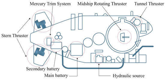
Figure 1.
Diagram of the deep-sea submersible’s schematic structure.
Table 2.
List of sensors related to the hydraulic and propulsion systems.
Central to our approach is the concept of the “coupling manifold,” . We formally define this as the low-dimensional manifold embedded within the fused latent space, which is populated by the joint latent representations corresponding to normal, healthy system operation. Mathematically, it can be expressed as:
where is the data distribution under normal conditions, and , . The DSC-AE training process is designed to learn the structure of this manifold. From a probabilistic perspective, represents the region of high probability density for the joint latent variable distribution. Any data point whose latent representation falls far from this manifold is considered anomalous.
3.1.2. Preliminary Analysis: System Coupling Evidence
Before introducing our proposed model, it is crucial to first quantitatively establish the presence of coupling between the hydraulic and propulsion systems from the operational data itself. While the physical coupling is understood from an engineering perspective, demonstrating its signature in the sensor data provides a direct, data-driven motivation for a cross-system diagnostic model.
To this end, we conducted a correlation analysis on a representative dataset from normal operations. We computed the Pearson correlation coefficient between all pairs of sensor signals, encompassing both subsystems. The resulting correlation matrix is visualized as a heatmap in Figure 2.
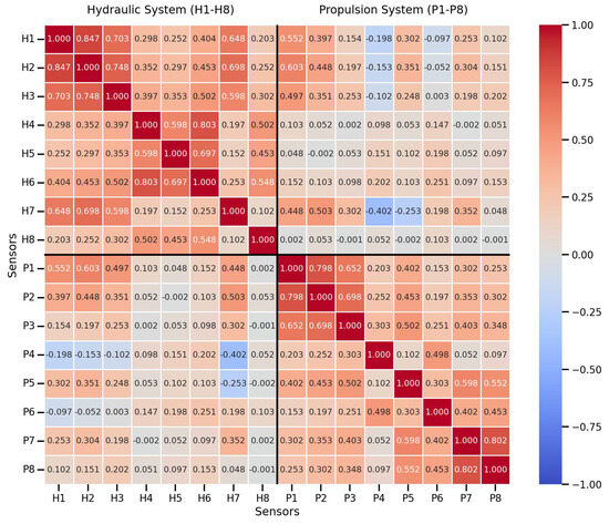
Figure 2.
Pearson correlation heatmap of all sensor signals from the hydraulic and propulsion systems, computed on data from normal operations.
As shown in Figure 2, the heatmap reveals several key patterns. The strong correlations along the diagonal blocks confirm high intra-system dependencies, as expected (e.g., various hydraulic pressures correlating with each other). More importantly, the off-diagonal blocks display numerous instances of non-trivial cross-system correlations. For example, we observe significant correlations between hydraulic pressure sensors (e.g., Sensor H1, H7) and propulsion sensors (e.g., Sensor P1, P2)—specifically, H1 correlates with P1 (0.552) and H7 correlates with P2 (0.503), directly reflecting cross-system dynamic links.
This quantitative evidence confirms that fluctuations in one system are statistically linked to the behavior of the other. However, linear correlation is insufficient to capture the full complexity of the underlying non-linear and time-varying dynamics. This finding strongly motivates the development of a more sophisticated, non-linear model, such as the proposed DSC-AE, which is specifically designed to learn these intricate coupling patterns for the purpose of anomaly detection.
3.2. Data Preprocessing
To ensure the quality and consistency of the model’s input data, we employed a multi-step preprocessing pipeline, as illustrated in Figure 3A, specifically tailored for the dual-system dataset. The pipeline consists of the following stages:
- Sensor Selection and Channel Formulation: Leveraging domain expertise, we selected key sensors from the submersible’s extensive sensor network that are most pertinent to the core functions of the hydraulic and propulsion systems. This resulted in the selection of eight sensors from the hydraulic system (detailed in Table 2) and eight from the propulsion system (including motor currents from the main ducted, midship, and stern thrusters, as well as mercury column pendulum readings). These sensors collectively constitute a 16-dimensional synchronized time-series data stream.
- Data Segmentation and Alignment: We isolated data segments corresponding to deep-sea cruising and operational phases by excising periods of pre-dive preparation and post-ascent recovery from the complete dive cycle recordings. Temporal synchronization across all sensor channels was ensured by aligning the data to a unified timestamp.
- Noise Filtering: To mitigate transient impulse noise attributable to the harsh deep-sea environment (e.g., hydrodynamic disturbances, sensor electrical interference), we applied a dual-filter strategy combining a moving median filter and an Interquartile Range (IQR) filter. This filtering process can be formally defined using a composite operator , which maps raw sensor data to cleaned data:where denotes the raw, unprocessed sensor time-series data, and represents the filtered data used for subsequent model input. Configured with a 60-s window size (matching the typical time scale of meaningful system dynamics) and an IQR multiplier of 1.5, effectively removes outlier values while preserving the integrity of genuine system state changes—laying the foundation for subsequent noise robustness in the model.
- Normalization: To eliminate the influence of disparate physical units (e.g., pressure, current) and value ranges on model training, we applied Z-score normalization to each sensor channel independently. For a given time-series channel with mean and standard deviation computed from the training set, each data point is transformed into as follows:
- Time-Window Segmentation: To capture the temporal dynamics of the systems, the continuous time series was segmented into overlapping samples using a sliding window approach. The window length T was set to 32 (corresponding to a 16-s duration), with a stride S of 16. This process transforms the data into a sequence of matrices, each with dimensions of , representing the synchronized readings of all 16 sensors (rows) over a 32-time-step interval (columns).
- Data Separation: To accommodate the dual-stream encoder architecture, each data window was partitioned along the sensor dimension into two sub-matrices: a matrix for the hydraulic system data comprising the first eight sensor channels (rows), and a matrix for the propulsion system data comprising the subsequent eight sensor channels (rows). Consequently, each training sample for the model consists of a time-synchronized tuple , where and .

Figure 3.
The overall pipeline and framework of the proposed cross-system anomaly detection method, encompassing three sequential stages: (A) data collection and pre-processing, (B) model training, and (C) fault tracing.
3.3. Dual-Stream Coupled Autoencoder Model
The architecture of the proposed Dual-Stream Coupled Autoencoder (DSC-AE) is founded on a Dual-Encoder, Single-Decoder (DE-SD) design, a choice fundamental to our goal of modeling inter-system coupling. This design was deliberately chosen over other possible configurations due to its superior capacity for learning the joint representation of healthy system behavior. Here, we provide a theoretical justification by comparing it with two logical alternatives.
Dual-Encoder, Single-Decoder (Proposed): This architecture, as depicted in Figure 3B, first employs two specialized encoders () to learn disentangled, system-specific latent representations (). The critical component is the single, shared decoder (D), which must reconstruct both original inputs () from the single fused vector . This structure forces the model to learn the conditional dependencies between the subsystems. For the decoder to successfully reconstruct the hydraulic state , for instance, it must leverage the information about the propulsion state contained within . Consequently, the training process compels the latent vectors and to align in a way that captures the mutual information inherent in normal, coupled operations. This effectively models the joint distribution .
- Alternative Configurations: We contrast our approach with two other designs:
- Separate Autoencoders (DE-DD): Using two fully independent autoencoders ( and ) would only model the marginal distributions and . This approach is fundamentally incapable of learning the coupling between systems and would fail to detect cross-system anomalies.
- Single-Encoder, Dual-Decoder (SE-DD): This configuration involves concatenating the inputs () into a single encoder. This “early fusion” approach learns a joint representation but struggles to disentangle subsystem-specific features from their interactions. As our results suggest (Section 5), this form of data-level fusion is less effective at distinguishing genuine fault propagation from benign responses, as the model may learn spurious correlations rather than the underlying physical coupling.
Our proposed DE-SD architecture uniquely allows the model to first learn robust, system-specific features before explicitly learning their coupling relationship through the shared reconstruction task, making it the most suitable for our problem. The following subsections detail the key components that constitute this architecture. manifold structure.
3.3.1. Dual-Stream Encoding Network
The model initially processes the preprocessed and separated hydraulic and propulsion system data using two independent, structurally identical encoders and . Each encoder, composed of convolutional and fully-connected layers, is designed to extract temporal features from its respective system efficiently. The hydraulic encoder takes the hydraulic system data as input, which contains the readings from eight critical hydraulic sensors (rows) over a 32-time-step window (columns). Similarly, the propulsion encoder takes the propulsion system data as input, containing synchronous readings from eight key propulsion sensors (rows) over the same 32-time-step window (columns).
The encoding process is formally defined as:
where are the latent space feature vectors corresponding to the hydraulic and propulsion system inputs, respectively. The use of CNN-based encoders facilitates the effective capture of local temporal patterns while reducing computational complexity. Additionally, the encoding process contributes to noise robustness through latent manifold projection. The encoders act as mappings from high-dimensional input space to the low-dimensional coupling manifold (defined in Section 3.1), formally expressed as:
By prioritizing features aligned with (which captures essential dual-system coupling dynamics), the encoders inherently filter out residual small-scale, high-frequency, or random noise components that lie “off-manifold.” This implicit denoising is driven by the model’s total objective function: the reconstruction loss term forces the encoder-decoder pipeline to retain only noise-free, reconstructible features, while the coupling loss reinforces alignment with . This complements the explicit noise filtering in preprocessing, enhancing the model’s resilience to real-world sensor noise.
3.3.2. Bottleneck Fusion Layer
To model the coupling relationships between the systems, the feature vectors extracted from the two systems are concatenated at the bottleneck layer, forming a fused, joint representation. This choice of concatenation is deliberate: it minimizes inductive bias by avoiding predefined assumptions (like linear or modulatory interactions) that alternative techniques impose. As an information-lossless operation, it preserves full features from both encoders, letting the shared decoder flexibly learn complex, non-linear inter-system couplings directly from data.
Here is the fused feature vector, which encodes the combined state information of both the hydraulic and propulsion systems within the time window.
3.3.3. Shared Decoder and Joint Reconstruction
The fused feature vector is fed into a shared decoder D for reconstruction. The role of this decoder is to simultaneously recover the original input data for both systems from their joint representation.
where and are the reconstructed outputs for the hydraulic and propulsion systems, respectively. By attempting to disentangle and reconstruct the data of both systems from a single joint feature vector, the shared decoder is compelled to learn the intrinsic mappings and dependencies between them.
3.3.4. Objective Function
The model is trained by optimizing a composite objective function designed to simultaneously achieve three goals: accurate data reconstruction, explicit enforcement of latent space coupling, and prevention of model overfitting. This total objective function, , is a weighted sum of three distinct loss components, each defined and explained below.
The primary objective of the model is to reconstruct the input data accurately. To this end, we define separate reconstruction losses for the hydraulic and propulsion subsystems. Each loss is measured using the Mean Squared Error (MSE) computed via the squared Frobenius norm, normalized by the number of sensors () and time steps (T) of the respective subsystem to ensure scale consistency:
Here, quantifies the reconstruction fidelity of the hydraulic system data, and quantifies that of the propulsion system data.
To explicitly model the inter-system dependencies and enforce the shared latent space assumption (a key requirement of the DSC-AE), we introduce a coupling loss. This loss minimizes the distance between the latent vectors (from the hydraulic encoder ) and (from the propulsion encoder ), compelling the two encoders to map coupled, normal system states to nearby points in the latent space. To ensure a precise mathematical formulation, we define the coupling loss using the squared L2 norm:
To prevent overfitting—especially critical for avoiding memorization of training data noise and ensuring generalization to unseen operational data—we incorporate an L2 regularization term (also known as weight decay). We provide its formal definition: this term penalizes large values of all trainable model parameters (including weights of encoders and decoder D), encouraging simpler model weights and more robust latent representations:
The final objective function combines the reconstruction, coupling, and regularization losses into a single, comprehensive loss that is minimized during training. Integrating all the above components, the total objective function is formulated as:
The non-negative hyperparameters and control the trade-off between the three core objectives, with distinct roles:
- and : Weighting coefficients for the hydraulic and propulsion reconstruction losses, respectively. They allow adjusting the relative importance of reconstruction fidelity for each subsystem (e.g., emphasizing one subsystem if its sensor data is more critical for anomaly detection).
- : Coupling coefficient that governs the strength of the penalty for latent vector divergence. A larger enforces tighter alignment between and , strengthening the modeling of inter-system coupling.
- : Regularization parameter that controls the intensity of weight decay. A larger imposes a stricter penalty on large parameters, reducing model complexity and overfitting risk.
3.4. Anomaly Detection and Fault Localization
The comprehensive framework for the proposed cross-system anomaly detection method is depicted in Figure 3, which encompasses three sequential stages: (A) data collection and pre-processing, (B) model training, and (C) fault traceability. This architecture is designed to holistically monitor the coupled hydraulic and propulsion systems by learning their joint behavior under normal conditions. During the training phase, the model is developed using only synchronized time-series data from healthy operations. In the subsequent inference phase, the trained model evaluates new data windows to compute an anomaly score based on reconstruction fidelity. If this score surpasses a determined threshold, an alarm is triggered, and the fault traceability module is activated to provide diagnostic insights.
The detailed training procedure for the Dual-Stream Coupled Autoencoder is presented in Algorithm 1. During this unsupervised learning phase, the model is optimized by minimizing the joint reconstruction error. This process compels the model to learn a compact and robust representation of the normal, coupled dynamics between the hydraulic and propulsion systems.
| Algorithm 1 Training procedure for the DSC-AE |
| Input: Training dataset , batch size B, hyperparameters α, β, γ, λ Output: Trained encoders , and decoder D 1: Initialize parameters 2: for each training iteration do 3: Sample a mini-batch from 4: Encode: , 5: Fuse: 6: Reconstruct: 7: Compute total batch loss : 8: Update all parameters based on : 9: end for |
Once the model is trained, the anomaly score for a new test sample is formally defined as the total reconstruction error, which aligns with the reconstruction loss component of our objective function:
This metric is particularly effective for detecting propagated faults. A fault originating in one subsystem will cause a high reconstruction error in that subsystem. As the fault affects the coupled dynamics, the behavior of the other subsystem will also deviate from the learned normal patterns, leading to an increase in its reconstruction error as well. The sum of these errors provides a single, sensitive metric that robustly captures deviations from the learned system-wide normality.
To determine if a sample is anomalous, its score is compared against a statistically derived threshold. This threshold (T) is established from the model’s own reconstruction error distribution on the normal training data, ensuring it is optimally tailored to the learned model of healthy operation. The calculation follows the standard three-sigma () rule:
- After training, all samples from the normal training set are passed through the finalized DSC-AE model to generate a population of normal-state anomaly scores .
- The mean () and standard deviation () of these anomaly scores are calculated:where N is the total number of time-window samples in the training set.
- The threshold T is then defined as:
Any sample with an anomaly score is flagged as anomalous, triggering the fault localization process. To identify the root cause of the anomaly, we calculate the average anomaly score for the k-th sensor, denoted as , is computed as:
where is the total number of time steps. To trace the fault’s origin and propagation, we compute the reconstruction error for each sensor channel across the time steps of the anomalous window, generating a reconstruction error heatmap. This heatmap, a matrix , visualizes the error distribution. Each element of the heatmap represents the point-wise reconstruction error for the k-th sensor at the t-th time step within a given window. It is formally defined as the absolute difference between the original and reconstructed values:
where is the value from the k-th sensor (row) at time step t (column) of the concatenated input matrix , and is its corresponding reconstructed value. Visual analysis of this heatmap allows for the intuitive identification of which sensors first exhibit high reconstruction errors, the duration of the anomaly, and its propagation path across different systems. This provides operators with rich, interpretable information for rapid diagnosis.
3.5. Computational Complexity Analysis
To evaluate the efficiency of the proposed DSC-AE model, we analyze its computational complexity in terms of both time (inference cost) and space (parameter storage). Let T be the time-window length, N be the number of sensor channels per system, K be the convolutional kernel size, and be the channel counts of the two convolutional layers, and d be the dimension of the latent space for a single encoder.
Time Complexity: The time complexity is determined by the number of floating-point operations (FLOPs) required for a single forward pass during inference. We analyze the complexity of each component as follows. For Encoders ( and ): since they are identical, we analyze one. The first 1D convolutional layer has a complexity of . The second has a complexity of . The final fully connected layer operates on the flattened feature map of size approximately and has a complexity of . For Shared Decoder (D): the first fully connected layer has a complexity of . The two subsequent transposed convolutional layers have complexities of and , respectively. The total time complexity is the sum of these components. Since the two encoders operate in parallel, the dominant operations are duplicated. The overall complexity is approximately . This shows that the model’s inference time scales linearly with the input window length T, which is an efficient property for real-time monitoring applications.
Space Complexity: The space complexity is determined by the number of trainable parameters in the model, which dictates the memory required to store it. We analyze the parameter count of each component as follows. For Encoders ( and ): the parameters are dominated by the convolutional kernels and the fully connected layer. The total parameters for one encoder are approximately . For Shared Decoder (D): the parameters are approximately . The total space complexity is the sum of parameters from both encoders and the shared decoder: . This value is fixed once the model architecture is defined and is independent of the size of the training or test dataset. For our specific architecture (Table 3), the flattened dimension before the latent space is 896, which is the primary contributor to the parameter count in the fully connected layers.
Table 3.
The detailed architecture of the DSC-AE model.
4. Experiments and Analysis
4.1. Evaluation Metrics
To quantitatively evaluate the anomaly detection performance, we use standard classification metrics based on the evaluation of each time-window sample. We first define the following terms by comparing model predictions against ground-truth labels:
- True Positive (TP): An anomalous sample correctly identified as an anomaly.
- False Positive (FP): A normal sample incorrectly identified as an anomaly.
- True Negative (TN): A normal sample correctly identified as normal.
- False Negative (FN): An anomalous sample incorrectly identified as normal.
Based on these counts, we compute Accuracy, Precision, Recall, False Positive Rate (FPR), and the F1-Score as follows:
Regarding the suggestion for propagation-aware variants, we acknowledge this as a valuable research direction. For the current study, we adhere to these widely accepted sample-wise metrics to ensure a fair and direct comparison with baseline methods.
4.2. Experimental Setup
The proposed method is validated on a real-world dataset collected from a deep-sea submersible during its operational missions. As detailed in Table 4, the dataset comprises sensor data from multiple dives, which are partitioned into training and testing sets based on their operational status. The training set consists of 21,440 time-window samples from five entirely normal dives (Dive 95, 107, 111, 135, and 150). This set is used to train all benchmark models to learn nominal operational patterns. The testing set encompasses data from six distinct dives to facilitate a comprehensive performance evaluation:
- Normal Data: Dive 70 (1260 samples), representing normal coupled system operation.
- Intra-System Faults: Dive 76 (1050 samples), featuring an internal oil leakage in the hydraulic system, and Dive 140 (980 samples), characterized by a magnetic coupling failure in the port-side stern thruster.
- Cross-System Faults: Dive 96 (1090 samples), where an internal leakage in a hydraulic pump led to performance degradation in a thruster, and Dive 146 (1150 samples), where a thruster bearing seizure induced a pressure surge in the hydraulic system.
- Synthetic Anomalies: Dive 93 (1360 samples). To precisely quantify model performance with known ground-truth, a dataset with synthetic anomalies was generated from a normal dive (Dive 93). Anomalies were injected by setting the readings of three randomly selected key sensor channels (System VP1 Pressure, Channel Thruster, and 100 V Power Supply Current) to zero for continuous, randomly chosen time segments, totaling 15% of the dive’s duration. This procedure simulates complete sensor failure or signal loss and provides a controlled benchmark for evaluating detection precision and recall.
Table 4.
List of datasets used in the experiments.
Table 4.
List of datasets used in the experiments.
| Set Type | Dive ID | Operational Status | Description |
|---|---|---|---|
| Training | Dive 95 | Normal | Healthy operational data for model training |
| Dive 107 | Normal | Healthy operational data for model training | |
| Dive 111 | Normal | Healthy operational data for model training | |
| Dive 135 | Normal | Healthy operational data for model training | |
| Dive 150 | Normal | Healthy operational data for model training | |
| Testing | Dive 70 | Normal | Healthy baseline for performance evaluation |
| Dive 76 | Intra-System Fault | Internal oil leakage in the hydraulic system | |
| Dive 140 | Intra-System Fault | Magnetic coupling failure in a propulsion thruster | |
| Dive 96 | Cross-System Fault | Hydraulic pump leak degrading thruster performance | |
| Dive 146 | Cross-System Fault | Thruster bearing seizure causing hydraulic pressure surge | |
| Dive 93 | Synthetic Anomaly | Controlled sensor failures for quantitative evaluation |
To ensure a fair comparison, we selected an Early-Fusion Autoencoder (EarlyFusion-AE) as a baseline model. This model adopts a direct fusion strategy where, at the input stage, the data from the hydraulic system () and the propulsion system () are concatenated along their feature (sensor) dimension. This process yields a single, unified input matrix . The resulting matrix is then fed into a standard, single-stream autoencoder for feature extraction and reconstruction. To maintain an equitable comparison, the architecture of this autoencoder is designed to have a parameter count comparable to that of the sub-networks in our proposed DSC-AE. The underlying assumption of this approach is that the model can autonomously learn the inter-system correlations directly from the raw, early-fused data.
All experiments were conducted on a workstation equipped with an NVIDIA GeForce RTX 4060 GPU (8GB VRAM), utilizing Python 3.9.18 and the PyTorch 1.13.1 framework. During data preprocessing, all time-series data were standardized using Z-score normalization, with parameters () computed on the training set (see Equation (3)). This centers each sensor channel around zero with unit variance, mitigating the influence of disparate value ranges and helping stabilize the training process by preventing features with larger numerical ranges from disproportionately affecting the model’s loss computation and gradient-based learning. The model architecture is detailed in Table 3, with an input dimension of ‘(8, 32)’ per system, corresponding to 8 sensor channels over 32 time steps. The symmetric encoders ( and ) each employ two 1D convolutional layers (kernel size = 3, stride = 1) that expand the channel count from 8 to 16 and then to 32, using LeakyReLU as the activation function with a negative slope of 0.1. Batch Normalization is applied after each convolutional layer to enhance training stability and convergence speed. The resulting feature maps are flattened and projected into 64-dimensional latent vectors. This dimension was not chosen arbitrarily but was guided by a data-driven mathematical criterion. Specifically, we performed Principal Component Analysis (PCA) on the training data, which revealed that approximately 56–58 principal components were required to capture over 99% of the variance in each subsystem’s data. By selecting a latent dimension of 64, we ensure the model has sufficient capacity to represent these core linear dynamics, while also providing the necessary freedom for the deep network to learn the non-linear relationships and cross-system couplings that PCA cannot capture. The shared decoder D receives the concatenated 128-dimensional vector and reconstructs the original input dimensions through a symmetric transposed convolutional structure, culminating in a Tanh activation layer.
The objective function consists of four key components: first, the reconstruction losses for the hydraulic () and propulsion () systems, with weights —this equal setting ensures an unbiased contribution of both subsystems to the loss, as there is no domain knowledge indicating one system is more critical for anomaly detection; second, a coupling loss () with a weight , chosen to emphasize cross-system dependencies while preserving the primary focus on accurate reconstruction of individual subsystems, aligning with our core goal of modeling inter-system coupling without overshadowing baseline reconstruction performance; third, a regularization loss () with a weight , which corresponds to the strength of L2 regularization—this value follows standard practices for models of this complexity, striking a balance between penalizing excessive weight magnitudes and retaining the model’s capacity to learn meaningful system dynamics. The model was trained using the Adam optimizer with a learning rate of and momentum parameters and . To mitigate overfitting and ensure the model learns a generalizable representation in the latent space, two key regularization techniques were employed. First, a Dropout layer with a rate of 0.1 was added after the convolutional layers in the encoders. This technique randomly deactivates neurons during training, which prevents the model from becoming overly reliant on any single feature and forces it to learn more robust, distributed representations. Second, the aforementioned L2 regularization (weight decay) of was applied, which penalizes large weights, discouraging the model from learning an overly complex function that simply “memorizes” the training data. Together, these methods ensure that the learned latent space is smooth and captures the true underlying dynamics of normal operation, rather than fitting to noise. This is critical for robust anomaly detection, as it leads to a lower false positive rate on unseen normal data. The training was performed with a batch size of 128 for 90 epochs, and the key hyperparameters are summarized in Table 5.
Table 5.
Training hyperparameters for the DSC-AE model.
4.3. Experimental Validation on Real-World Data
To validate the proposed Coupled Dual-Stream Autoencoder, or DSC-AE, we conducted a comprehensive evaluation on real-world operational datasets. Its performance was systematically benchmarked against an early-fusion autoencoder, hereafter referred to as AE, to verify its superior efficacy in diagnosing complex cross-system faults. The baseline AE model employs a direct concatenation strategy, fusing the hydraulic data and propulsion data along the feature dimension to form a single input matrix, , which simplifies to . This unified matrix is then processed by a standard autoencoder, whose architecture has a parameter count comparable to the sub-networks within our DSC-AE. The foundational premise of this baseline is that the model can autonomously learn inter-system correlations from the raw, fused data.
4.3.1. Analysis of Normal Operation and Intra-System Faults
Under normal operating conditions in Dive 70, both models yielded low anomaly scores, indicating a minimal false-positive rate as detailed in Table 6. The DSC-AE model achieved a marginally lower mean score of compared to the baseline AE’s . This suggests our model’s enhanced generalization to healthy synergistic operations by more accurately modeling the normal inter-system coupling. The low-intensity reconstruction error heatmap in Figure 4a visually confirms this stable state.
Table 6.
Comparison of anomaly scores (mean ± standard deviation) across dive test datasets.
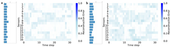
Figure 4.
Distribution of mean anomaly scores per sensor and heatmap of reconstruction errors for representative data blocks in normal test dataset: (a) Dive 70 (Normal), DSC-AE; (b) Dive 70 (Normal), AE.
To establish a robust and principled threshold for anomaly detection, we applied the methodology described in Section 3.4. Using the reconstruction error distribution of our DSC-AE model on the entire normal training dataset, we calculated the mean () and standard deviation (). This results in an anomaly detection threshold of:
This value, which theoretically encompasses 99.7% of all normal operational fluctuations as captured by our model, was used as the anomaly baseline for all subsequent fault detection experiments.
For intra-system faults, both models demonstrated effective detection capabilities. In Dive 76, a hydraulic oil leakage event, both DSC-AE and AE registered high anomaly scores and correctly identified sensors 1 and 7 as the primary contributors, a finding consistent with the fault’s physical mechanism, as shown in Figure 5a,b. Similarly, during the thruster malfunction in Dive 140, both models effectively isolated the anomaly to sensor 13, the stern left thruster current, accurately pinpointing the fault’s origin, as shown in Figure 5c,d. These tests confirm that both architectures are competent at identifying faults confined to a single subsystem.
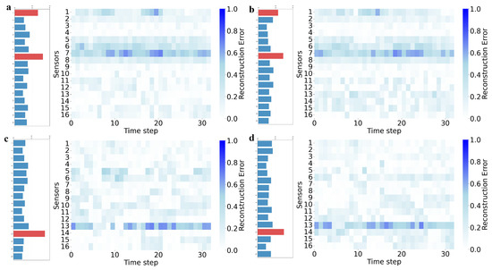
Figure 5.
Distribution of mean anomaly scores per sensor and heatmap of reconstruction errors for representative data blocks in intra-system fault test dataset: (a) Dive 76, DSC-AE; (b) Dive 76, AE; (c) Dive 140, DSC-AE; (d) Dive 140, AE.
4.3.2. Diagnosis of a Cross-System Fault Originating in the Hydraulic System
The scenario in Dive 96 involved a subtle cross-system fault, where an internal leakage in a hydraulic pump led to the performance degradation of a thruster. Both models successfully detected the anomaly, with DSC-AE and AE reporting high mean scores of and , respectively, as listed in Table 6. The sensor-wise score distributions in Figure 6a,b reveal that both models correctly implicated sensors from both subsystems, namely sensor 1 and 7 from the hydraulic system and sensor 12 from the propulsion system.
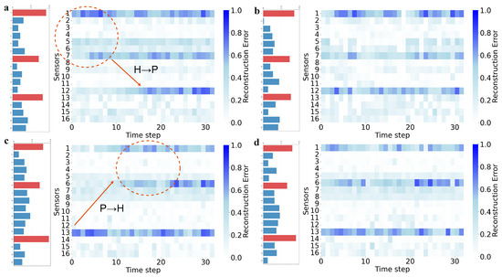
Figure 6.
Distribution of mean anomaly scores per sensor and heatmap of reconstruction errors for representative data blocks in cross-system fault test dataset: (a) Dive 96, DSC-AE; (b) Dive 96, AE; (c) Dive 146, DSC-AE; (d) Dive 146, AE.
The critical distinction between the models emerges from the temporal dynamics of their reconstruction errors, illustrated in the heatmaps of Figure 6a,b. The DSC-AE heatmap reveals a clear temporal sequence: errors first escalate persistently on hydraulic sensors 1 and 7, after which a significant error rise appears on propulsion sensor 12. This pattern visually reconstructs the fault propagation pathway from the hydraulic system to the propulsion system. In contrast, the AE’s heatmap shows high errors on the same sensors but depicts them as temporally concurrent and disordered, offering no insight into the causal chain of events.
This diagnostic sequence precisely mirrors the underlying physical process. The fault originated with an internal pump leakage, which caused pressure fluctuations in the hydraulic system, monitored by sensors 1 and 7. This instability then starved the mid-hull right thruster of adequate hydraulic power, leading to its performance decay, which was registered by sensor 12. The ability of DSC-AE to resolve this temporal propagation, a feat unattainable by the standard AE, underscores its unique advantage in root cause analysis for interconnected systems, aligning perfectly with post-dive maintenance findings.
4.3.3. Diagnosis of a Cross-System Fault Originating in the Propulsion System
Dive 146 presented a different cross-system fault, where a thruster bearing seizure induced a severe pressure shock in the hydraulic system. The DSC-AE model again registered a high anomaly score of , slightly higher than the AE’s . As shown in Figure 6c,d, both models correctly identified sensor 13 from the propulsion system and sensors 1 and 6 from the hydraulic system as the most anomalous channels.
Once again, the heatmaps provide a deeper comparative insight. The DSC-AE’s heatmap in Figure 6c compellingly illustrates the fault’s true origin and trajectory. A dramatic error spike first appears on sensor 13, the thruster current, followed by an explosive error burst on sensor 1, the main system pressure, and a subsequent gradual error increase on sensor 6, the oil tank temperature. This temporal sequence strongly indicates a fault that originated in the propulsion system and propagated catastrophically to the hydraulic system. The AE’s heatmap, however, again displays temporally overlapping and ambiguous errors across these sensors, obscuring the propagation pathway.
The physical events of this fault confirm the DSC-AE’s diagnostic narrative. The root cause was a mechanical seizure in the stern left thruster, causing an immediate current surge detected by sensor 13. This immense mechanical load propagated back into the hydraulic circuit, inducing a pressure shock and temperature rise captured by sensors 1 and 6. The DSC-AE model’s ability to capture this causal chain, from thruster seizure to hydraulic system impact, validates its effectiveness. The AE’s failure to do so further highlights how simple data fusion strategies are insufficient for deciphering the complex fault dynamics in coupled systems.
4.3.4. Summary of Diagnostic Performance
The experimental results conclusively demonstrate that the proposed DSC-AE model offers significant advantages beyond superior detection performance. Its most critical contribution lies in its unique ability to distinguish fault origins and reveal propagation pathways in coupled systems. While the baseline AE model can detect the presence of anomalies, its monolithic fusion architecture struggles to learn the intricate, normal coupling relationships between subsystems. This limitation causes it to generate a convoluted error representation where the effects of a fault appear as temporally disordered events, precluding any meaningful root cause analysis.
In contrast, the DSC-AE’s dual-stream architecture, coupled with its joint reconstruction mechanism, is explicitly designed to model the normal mapping between the hydraulic and propulsion systems. This architectural choice makes it highly sensitive to deviations from these learned healthy dynamics. As a result, the model not only detects faults with high accuracy but also provides causally informative diagnostic insights through the spatio-temporal distribution of its reconstruction errors. This capability to deconstruct a complex system failure into a clear, interpretable sequence of events represents a substantial advancement in intelligent fault diagnosis for complex engineered systems.
4.4. Comparative Experiments and Analysis
To systematically validate the proposed DSC-AE framework, we conducted a comprehensive set of experiments on the Dive 93 test set, which features synthetically generated anomalies. Our evaluation is twofold: first, we benchmark DSC-AE against a diverse set of established anomaly detection methods; second, we conduct a dedicated ablation study to isolate and quantify the contribution of our proposed bottleneck fusion architecture. The performance of all models is evaluated across four key metrics: accuracy, recall, False Positive Rate (FPR), and F1-score. To ensure a fair comparison, all deep learning models were configured with comparable parameter counts and trained under identical experimental protocols.
4.4.1. Comparison with Baseline Methods
We first compare the performance of DSC-AE against three representative baseline methods from different categories:
- Principal Component Analysis (PCA): A classical linear dimensionality reduction technique.
- One-Class Support Vector Machine (OC-SVM): A widely-used kernel-based approach.
- LSTM-AE: A state-of-the-art deep learning model for sequential data that processes the concatenated input from both subsystems.
As presented in Table 7, the quantitative results highlight the limitations of conventional methods in handling the complex, non-linear dynamics of our cross-system data. PCA, being a linear method, demonstrated the weakest performance. While OC-SVM and LSTM-AE offered significant improvements, they struggled to achieve a good balance between recall and false positives. The LSTM-AE, despite its high recall, exhibited a relatively high FPR (0.087), suggesting that simply processing concatenated sequences is insufficient to distinguish genuine faults from benign operational couplings.
Table 7.
Quantitative comparison of anomaly detection performance on the synthetic test dataset.
In stark contrast, our proposed DSC-AE achieved the most balanced and superior performance, attaining the highest F1-Score of 0.907. This is achieved by maintaining an excellent recall (0.901) while simultaneously achieving the lowest FPR (0.041) among all methods. This outcome strongly supports our central hypothesis: explicitly modeling the normal coupling between subsystems establishes a more precise and robust boundary for normal system behavior, leading to superior detection capabilities.
4.4.2. Ablation Study on Fusion Strategy
To specifically quantify the contribution of our proposed dual-stream bottleneck fusion architecture, we conducted a dedicated ablation study. We compared our full DSC-AE model against a strong baseline, the Autoencoder (AE), which can be seen as an ablated version of our model. The AE implements a simple data concatenation (early-fusion) strategy, where data from both subsystems are fused at the input level before being processed by a standard autoencoder. This direct comparison is designed to isolate the effect of our bottleneck fusion mechanism against a more naive fusion approach.
The results, presented in Table 8, provide clear quantitative evidence for the superiority of our bottleneck fusion strategy. While the early-fusion AE achieves a respectable F1-score of 0.842, our DSC-AE significantly boosts this to 0.907. Crucially, this improvement is largely driven by a 56% reduction in the False Positive Rate (FPR) (from 0.094 to 0.041), while also slightly increasing recall.
Table 8.
Ablation study comparing the proposed bottleneck fusion (Ours) against early fusion (AE).
To offer a more intuitive and qualitative insight into this performance gap, we visualized the distribution of anomaly scores for both normal and abnormal test data using t-SNE, as shown in Figure 7. This visualization powerfully illustrates the discriminative capability of each model. For the baseline AE (Figure 7a), there is a considerable overlap between the score distributions of normal (blue) and anomalous (red) data. This ambiguity in the decision space directly explains its higher false positive rate, as the model struggles to consistently separate benign operational fluctuations from genuine faults. In stark contrast, our DSC-AE (Figure 7b) demonstrates a much clearer and more distinct separation between the two classes, forming two well-defined clusters. This indicates that our model maps normal and anomalous states to a more discriminative feature space.
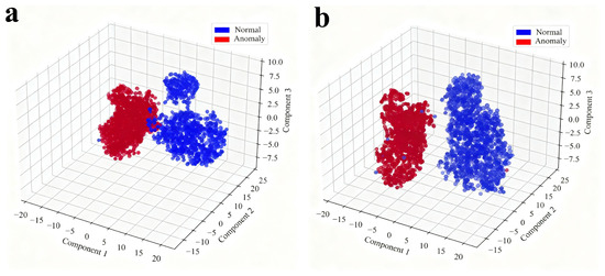
Figure 7.
Distribution of Scores for Normal and Abnormal Data: (a) AE; (b) DSC-AE.
Taken together, both the quantitative metrics and the score distribution visualization empirically validate our central hypothesis: fusing features at the semantic latent level, after they have been processed by specialized encoders, allows the model to learn the underlying physical coupling more effectively. This enhanced understanding enables the DSC-AE to distinguish genuine fault propagation from benign inter-system responses with much higher confidence. This study confirms that our dual-stream bottleneck fusion is a critical component for achieving robust and reliable anomaly detection performance.
4.4.3. Statistical Significance Analysis
While the mean performance metrics in Table 7 are indicative, it is crucial to verify that the observed superiority of our DSC-AE model is statistically significant and not a product of random experimental variation. To this end, we conducted a formal statistical hypothesis testing.
We used the F1-scores from the 10 independent runs described in Section 4.4.1 as our data samples. We performed the Wilcoxon signed-rank test, a non-parametric paired test, to compare the F1-score distribution of our model against each of the four baseline methods. The null hypothesis () for each test posits that there is no significant difference between the performance of the two compared models. The results of these tests are summarized in Table 9.
Table 9.
Results of the Wilcoxon signed-rank test for F1-scores on the ‘Dive 93’ test set (N = 10 runs). Significance level = 0.05.
As detailed in Table 7, the p-values for all comparison pairs are substantially lower than the significance level of = 0.05. For instance, the comparison against PCA yields a p-value less than 0.001, indicating an extremely significant difference. Even when compared against the strongest baseline, LSTM-AE, the p-value of 0.006 provides strong evidence to reject the null hypothesis. Therefore, we can conclude with high statistical confidence that the proposed DSC-AE model provides a significant improvement in anomaly detection performance over all tested baseline methods.
5. Conclusions
5.1. Research Summary and Contributions
In this paper, we addressed the critical challenge of diagnosing cross-system faults in deep-sea submersibles, where strong inter-system coupling can mask fault signatures and mislead traditional diagnostic models. We proposed and developed the Dual-Stream Coupled Autoencoder (DSC-AE), a novel deep learning framework designed to learn the intrinsic coupling patterns between the hydraulic and propulsion systems during normal operations. By employing a specialized dual-encoder, single-decoder architecture, our model moves beyond isolated system monitoring to establish a comprehensive, system-wide reference for healthy behavior.
Our extensive experimental evaluation, conducted on real-world mission data from the deep-sea manned submersible, has clearly demonstrated the superiority of our approach. The DSC-AE not only achieved significantly higher accuracy in detecting complex cross-system anomalies compared to conventional and deep learning baselines but also proved remarkably effective at identifying localized intra-system faults. This outcome strongly validates our central hypothesis: explicitly modeling the normal coupling between subsystems establishes a more precise and robust boundary for normal system behavior. A key practical advantage of our framework is its inherent interpretability; the analysis of reconstruction error heatmaps provides a clear, visual, and intuitive method for tracing fault propagation paths back to their source—a feature of immense value for operational diagnostics and post-mission maintenance.
The core principle of the DSC-AE—learning a representation of normal inter-system coupling rather than just individual system behavior—represents a promising paradigm for health management in other complex cyber-physical systems. Its applicability extends beyond submersibles to any domain where component interdependencies are critical, such as aerospace vehicles, integrated power grids, and multi-robot collaborative platforms.
5.2. Limitations and Future Work
While this study demonstrates the effectiveness of the DSC-AE framework, we acknowledge several limitations that pave the way for future research. Future work will extend this study in three primary directions.
First, we will address framework scalability and deployment. Our current work focuses on two subsystems, but the core principles are generalizable. As formalized below, the DSC-AE can be extended to an n-stream model: for n subsystems with inputs , n parallel encoders generate latent vectors . The fused latent vector is fed to a shared decoder that reconstructs all inputs . The objective function is correspondingly generalized by summing reconstruction losses, , and extending the coupling loss to minimize the distance of each latent vector from their joint mean, . Future work will involve implementing and validating this n-stream architecture on more complex systems (e.g., integrating power and control systems) and exploring real-time deployment optimizations like model quantization and pruning to enhance computational efficiency.
Second, we will investigate mode-aware architectures to explicitly model varying operational regimes. The operational profile of the submersible is not monolithic, encompassing distinct phases like descent, cruising, and manipulation. While our current model successfully learns a generalized manifold of normal behavior across these modes, a more sophisticated approach could enhance sensitivity and interpretability. Future work could explore frameworks such as a Mixture-of-Experts (MoE) or regime-switching models. Such an architecture would learn a set of mode-specific “sub-manifolds,” potentially enabling more precise anomaly detection and providing valuable context (i.e., identifying the operational mode in which a fault occurs). This represents a promising path toward creating more adaptive and context-aware diagnostic systems.
Third, to enhance diagnostic rigor and robustness, we will formalize the analysis of fault propagation pathways. While the current heatmap approach offers strong intuitive evidence, we plan to develop a quantitative framework using methods like Granger causality or dynamic directed graphs to enable a more objective, automated approach to root cause analysis. Furthermore, we will investigate the model’s robustness to significant sensor noise and missing data, potentially by incorporating techniques from denoising or masked autoencoders.
Finally, to address the practical challenge of data scarcity and further substantiate the model’s interpretability, we will explore the use of transfer learning, where pre-trained encoders can be fine-tuned for new vehicles with limited data. We also plan to conduct a deep mathematical analysis of the learned latent space, employing visualization tools and quantitative metrics like clustering or manifold distance to rigorously verify the structure of the “coupling manifold” and its ability to separate normal from anomalous states. This will provide a deeper, model-centric understanding of the features learned by the DSC-AE.
Author Contributions
Conceptualization, X.F. and X.T.; methodology, X.T. with guidance from X.F.; validation, C.Z. and X.G.; formal analysis, X.T. and Z.H.; investigation, X.T., C.Z. and X.G.; writing—original draft preparation, X.T.; writing—review and editing, X.F., X.T. and C.Z.; supervision, X.F.; project administration, X.F.; funding acquisition, X.F. All authors have read and agreed to the published version of the manuscript.
Funding
This research was funded by the National Natural Science Foundation of China, grant number: 62273165.
Data Availability Statement
The data supporting the results of this study are available upon request from the corresponding author.
Conflicts of Interest
Author Xiang Gao was employed by the National Deep Sea Center. The remaining authors declare that the research was conducted in the absence of any commercial or financial relationships that could be construed as a potential conflict of interest.
References
- Dearden, R.; Ernits, J. Automated fault diagnosis for an autonomous underwater vehicle. IEEE J. Ocean. Eng. 2013, 38, 484–499. [Google Scholar] [CrossRef]
- Ma, X.; Wu, J.; Xue, S.; Yang, J.; Zhou, C.; Sheng, Q.Z.; Xiong, H.; Akoglu, L. A comprehensive survey on graph anomaly detection with deep learning. IEEE Trans. Knowl. Data Eng. 2021, 35, 12012–12038. [Google Scholar] [CrossRef]
- Li, J.; Yang, W.; Qiao, S.; Gu, Z.; Zheng, B.; Zheng, H. Self-supervised marine organism detection from underwater images. IEEE J. Ocean. Eng. 2025, 50, 120–135. [Google Scholar] [CrossRef]
- Davari, N.; Aguiar, A.P. Real-time outlier detection applied to a doppler velocity log sensor based on hybrid autoencoder and recurrent neural network. IEEE J. Ocean. Eng. 2021, 46, 1288–1301. [Google Scholar] [CrossRef]
- Zhou, D.; Zhao, Y.; Wang, Z.; He, X.; Gao, M. Review on diagnosis techniques for intermittent faults in dynamic systems. IEEE Trans. Ind. Electron. 2019, 67, 2337–2347. [Google Scholar] [CrossRef]
- Vaswani, N.; Chi, Y.; Bouwmans, T. Rethinking PCA for modern data sets: Theory, algorithms, and applications. Proc. IEEE 2018, 106, 1274–1276. [Google Scholar] [CrossRef]
- Schölkopf, B.; Platt, J.C.; Shawe-Taylor, J.; Smola, A.J.; Williamson, R.C. Estimating the support of a high-dimensional distribution. Neural Comput. 2001, 13, 1443–1471. [Google Scholar] [CrossRef]
- Auger, F.; Hilairet, M.; Guerrero, J.M.; Monmasson, E.; Orlowska-Kowalska, T.; Katsura, S. Industrial applications of the kalman filter: A review. IEEE Trans. Ind. Electron. 2013, 60, 5458–5471. [Google Scholar] [CrossRef]
- Ren, Z.; Lin, T.; Feng, K.; Zhu, Y.; Liu, Z.; Yan, K. A systematic review on imbalanced learning methods in intelligent fault diagnosis. IEEE Trans. Instrum. Meas. 2023, 72, 3508535. [Google Scholar] [CrossRef]
- Kim, G.; Choo, Y. Enhancing generalization of active sonar classification using semisupervised anomaly detection with multisphere for normal data. IEEE J. Ocean. Eng. 2024, 49, 1530–1548. [Google Scholar] [CrossRef]
- Radhakrishnan, A.; Beaglehole, D.; Pandit, P.; Belkin, M. Mechanism for feature learning in neural networks and backpropagation-free machine learning models. Science 2024, 383, 1461–1467. [Google Scholar] [CrossRef]
- Tao, X.; Gong, X.; Zhang, X.; Yan, S.; Adak, C. Deep learning for unsupervised anomaly localization in industrial images: A survey. IEEE Trans. Instrum. Meas. 2022, 71, 5018021. [Google Scholar] [CrossRef]
- Amarbayasgalan, T.; Pham, V.H.; Theera-Umpon, N.; Ryu, K.H. Unsupervised anomaly detection approach for time-series in multi-domains using deep reconstruction error. Symmetry 2020, 12, 1251. [Google Scholar] [CrossRef]
- Ruff, L.; Kauffmann, J.R.; Vandermeulen, R.A.; Montavon, G.; Samek, W.; Kloft, M.; Dietterich, T.G.; Muller, K.-R. A unifying review of deep and shallow anomaly detection. Proc. IEEE 2021, 109, 756–795. [Google Scholar] [CrossRef]
- Creswell, A.; Bharath, A.A. Denoising adversarial autoencoders. IEEE Trans. Neural Netw. Learn. Syst. 2018, 30, 968–984. [Google Scholar] [CrossRef]
- Sun, J.; Wang, X.; Xiong, N.; Shao, J. Learning sparse representation with variational auto-encoder for anomaly detection. IEEE Access 2018, 6, 33353–33361. [Google Scholar] [CrossRef]
- Alsulami, A.A.; Abu Al-Haija, Q.; Alqahtani, A.; Alsini, R. Symmetrical simulation scheme for anomaly detection in autonomous vehicles based on LSTM model. Symmetry 2022, 14, 1450. [Google Scholar] [CrossRef]
- Lu, W.; Li, Y.; Cheng, Y.; Meng, D.; Liang, B.; Zhou, P. Early fault detection approach with deep architectures. IEEE Trans. Instrum. Meas. 2018, 67, 1679–1689. [Google Scholar] [CrossRef]
- Khanmohammadi, F.; Azmi, R. Time-series anomaly detection in automated vehicles using D-CNN-LSTM autoencoder. IEEE Trans. Intell. Transp. Syst. 2024, 25, 9296–9307. [Google Scholar] [CrossRef]
- Zhang, Y.; Lei, Y. Data anomaly detection of bridge structures using convolutional neural network based on structural vibration signals. Symmetry 2021, 13, 1186. [Google Scholar] [CrossRef]
- Wijaya, K.T.; Paek, D.-H.; Kong, S.-H. Advanced feature learning on point clouds using multi-resolution features and learnable pooling. Remote. Sens. 2024, 16, 1835. [Google Scholar] [CrossRef]
- Deng, X.; Xiao, L.; Liu, X.; Zhang, X. One-dimensional residual GANomaly network-based deep feature extraction model for complex industrial system fault detection. IEEE Trans. Instrum. Meas. 2023, 72, 3520013. [Google Scholar] [CrossRef]
- Fang, X.; Zhao, Z.; Zhang, C.; Gao, X.; Ahn, C.K. Data-driven propulsion system fault diagnosis for deep-sea submersible. IEEE Internet Things J. 2025, 12, 43696–43706. [Google Scholar] [CrossRef]
- Gao, S.; Feng, C.; Wang, B.; Yan, T.; He, B.; Zio, E. Data and model combined unsupervised fault detection and assessment framework for underwater thruster. IEEE Trans. Ind. Inform. 2024, 20, 8229–8238. [Google Scholar] [CrossRef]
- Zhang, S.; Pattipati, K.R.; Hu, Z.; Wen, X.; Sankavaram, C. Dynamic coupled fault diagnosis with propagation and observation delays. IEEE Trans. Syst. Man, Cybern. Syst. 2013, 43, 1424–1439. [Google Scholar] [CrossRef]
- Wu, Y.; Dai, H.-N.; Tang, H. Graph neural networks for anomaly detection in industrial internet of things. IEEE Internet Things J. 2021, 9, 9214–9231. [Google Scholar] [CrossRef]
- Chen, Z.; Cheng, J.; Amiri, H.; Nagm, K.; Lin, L.; Sun, X.; Tolomei, G. Frog: Fair removal on graphs. arXiv 2025, arXiv:2503.18197. [Google Scholar] [CrossRef]
- Nan, X.; Zhang, B.; Liu, C.; Gui, Z.; Yin, X. Multi-modal learning-based equipment fault prediction in the internet of things. Sensors 2022, 22, 6722. [Google Scholar] [CrossRef]
- Zhang, Z.; Yao, Y.; Hutabarat, W.; Farnsworth, M.; Tiwari, D.; Tiwari, A. Time series anomaly detection in vehicle sensors using self-attention mechanisms. IEEE Trans. Intell. Transp. Syst. 2024, 25, 15964–15976. [Google Scholar] [CrossRef]
Disclaimer/Publisher’s Note: The statements, opinions and data contained in all publications are solely those of the individual author(s) and contributor(s) and not of MDPI and/or the editor(s). MDPI and/or the editor(s) disclaim responsibility for any injury to people or property resulting from any ideas, methods, instructions or products referred to in the content. |
© 2025 by the authors. Licensee MDPI, Basel, Switzerland. This article is an open access article distributed under the terms and conditions of the Creative Commons Attribution (CC BY) license (https://creativecommons.org/licenses/by/4.0/).