Abstract
Symmetry and anti-symmetry appear naturally in the study of systems of nonlinear equations resulting from numerous fields. The solutions of such equations can be obtained in analytical form only in some special situations. Therefore, algorithms or iterative schemes are mostly studied, which approximate the solution. In particular, Jarratt-like methods were introduced with convergence order at least six in Euclidean spaces. We study the methods in the Banach-space setting. Semilocal convergence is studied to obtain the ball containing the solution. The local convergence analysis is performed without the help of the Taylor series with relaxed differentiability assumptions. Our assumptions for obtaining the convergence order are independent of the solution; earlier studies used assumptions involving the solution for local convergence analysis. We compare the methods numerically with similar-order methods and also study the dynamics.
1. Introduction
Nonlinear equations (NEs) arise in science and engineering when modeling problems using mathematical modeling [1,2,3]. Many problems on symmetry properties which belong to different areas of science and engineering like quantum mechanics, cosmology, data analysis, operational research, finance, biology, etc. [4,5,6], have been converted into NEs in the literature. Since it is difficult to obtain the analytic solution of the NEs for most of the problems, iterative methods are used to find approximations for the solution [7,8]. For obtaining better approximations, researchers in this area are interested in developing efficient iterative methods [2,3,9,10,11,12,13,14,15,16]. A prototype for the iterative method was the celebrated Newton’s method (NM) [17]. Extensions of NM have been [17,18,19] developed for solving univariate as well as multivariate equations.
The order of convergence (OC) is an important measure that depicts the speed of convergence of a method. A sequence converges to with OC [20] if there exists a constant such that
Let be a nonlinear operator between the Banach spaces X and Y and be an open convex subset of X. Consider the NE
with a solution In [21], a Jarratt-like method based on a weight function was proposed to approximate The method was defined and analyzed in scalar and in Euclidean space settings only. We present a general version of this method, which is defined as follows:
Let , for ,
where (the set of all bounded linear operator from X into Y) satisfies the following properties:
and
where . An extension of the method which is of sixth order is defined as follows:
The analysis in [21] has the following limitations:
- ()
- The method is defined only for functions on .
- (
- The OC of the method is proved using Taylor series expansion, and to proceed with this, one needs the existence of derivatives of Ş up to order five and seven for methods (3) and (5), respectively.Let be such that
- ()
- One cannot predict the number of iterates required to reach a desired accuracy.
- ()
- The weight function Q needs to be differentiable at least four times.
In our analysis, by using the mean value theorem (MVT) as the key we enhance the applicability of the method. The main advantages of our analysis are as follows:
- ()
- The method is presented in the Banach-space setting.
- ()
- OC is obtained using assumptions on the first three derivatives of Ş.
- ()
- The class of weight function can be updated because we need conditions only until the second derivative of Q to prove the convergence order.
- ()
- The number of iterates needed to reach a desired accuracy can be predicted using our approach.
Another advantage of our analysis is that our assumptions for the local convergence analysis do not depend on the unknown solution . In earlier studies [22], two sets of assumptions were used, one set of assumptions for semilocal convergence analysis and another for local convergence analysis. We use the same set of assumptions for semilocal and local convergence analysis.
It is possible to increase OC by increasing the number of steps in the iteration method. There is a measure called the Efficiency Index (EI) [23,24,25] to calculate the efficiency of the method.
According to Ostrowski [25], the EI is given by
here R is the OC and where the number of function evaluations per iteration and the number of derivative evaluations per iteration.
The paper is arranged as follows. Section 2 deals with the semilocal convergence of the method (5). [The semilocal convergence of the method was already presented in ([22], Chapter 34) with two particular choices of Q. In this paper, we present the general version of the semilocal convergence with a slight modification in the analysis]. In Section 3, a local analysis of method (3) is presented and in Section 4, we provide a local analysis of method (5). Section 5 deals with the numerical examples and Section 6 contains the dynamics of the method. The paper ends with conclusions in Section 7.
2. Semilocal Convergence of Method (5)
We develop scalar majorizing sequences for our semilocal analysis [26]. We define the scalar sequences , , and using two constants: and . For , define
Lemma 1.
Proof.
Consider and .
Now, assume the following:
- There exist an initial point and a constant such that .
- There exist an operator and withSet .
- There exists with
- The condition (9) holds for .
- .
Remark 1.
- The choices for can be (the identity operator) or . If and are satisfied, then other choices are possible.
- From we have
Theorem 1.
Assume the conditions hold. Then, defined in (5) converges to , with .
Proof.
First, we prove the following assertions:
and
We use mathematical induction to prove the result. Using we obtain
And by the assumptions of Lemma 1 we have
Let . By we have
Hence, by the Banach lemma (BL) on an invertible operator [26], we obtain and
Note that by (15) we can obtain
So by the Banach lemma we obtain
Now, let us define
and using mean value theorem (MVT) and the identity , we can write
Since , from (20) we obtain
Again, use MVT on the above equation to obtain
Now, use the identity to obtain
Also, we have
and
Taking the norm on both sidess of the above equation and using the inequality (4), we obtain
Now, from the and substeps of (5) we have
Again, by using , (16) and (17), we have
Now, by using MVT and the fact that we obtain
then by using (10) we obtain
Now, from the substep of (5) we obtain
and using the identity we obtain
Now, using (10), we obtain
and using (33), (34), (16), (8), and we obtain
also
Finally, if we replace in the above estimates by , respectively, we can see the induction hypothesis is satisfied. [Notice that while replacing by , in all the places using assumption , the second in remains as itself. Also, in (27), (32), and (36), remains as itself].
Therefore, from (37)–(39) we can claim that for all . By condition and Lemma 1, the sequences , , and are Cauchy, and by (11)–(13) we have
so that sequences , , and are also Cauchy, and converge to some . Again, consider (34), since the induction holds we have
Finally, by the continuity of F, if we allow in the above inequality, we obtain . □
Remark 2.
Next, a region is given which contains only one solution of
Proposition 1.
Suppose the following exist:
- (i)
- A solution for some
- (ii)
- such thatSet Then, z is the unique solution of in the region
Proof.
See [19]. □
3. Local Analysis of (3)
We usethe following additional assumptions.
- , , .
- , , .
- for some and .
- for some and .
- for some and .
From Remark 2, we obtained . Then, by () we can observe that for ,
Now, using BL and (40) we obtain, for all , that is invertible and
Now, consider the functions, as non-decreasing and continuous and defined as
and
Then, and .
By intermediate value theorem (IVT) ∃ such that .
Further, let be non-decreasing and continuous functions defined as
and
Note that, and ; so, by IVT there exist the smallest zero for in defined by r, with .
We use the following inequalities in our study. For all by MVT, we obtain
By (41) and (), for we obtain
Using (42), we can find an estimation for provided , as follows:
Remark 3.
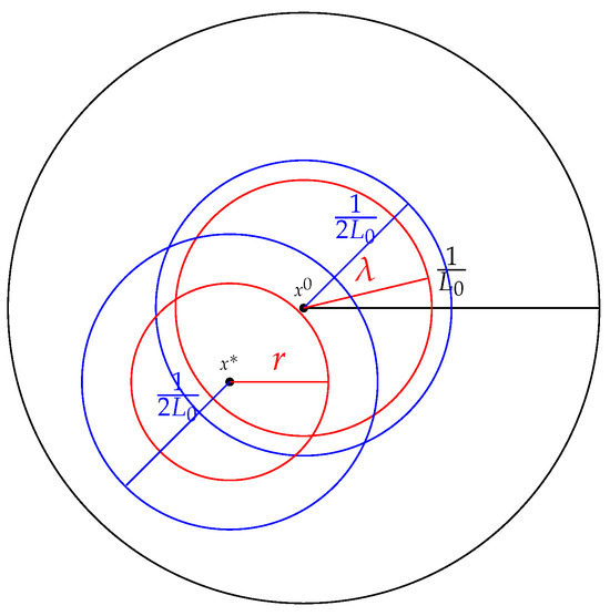
Note that the initial point we are considering in the local analysis is not the same as what we considered in the semilocal analysis. From now, we consider the in the semilocal analysis as a fixed element in Ω. We study the local convergence in , which satisfies
see Figure 1.
Figure 1.
Graphical representation of various balls considered.
Consequently, all the assumptions we considered are valid in the local convergence ball, so that we can proceed with the local analysis as an independent analysis with the same assumptions.
Theorem 2.
If assumptions , and ()–() hold. Then, the sequence defined by (3) with is well defined and
In particular, for all and converges to with OC four.
Proof.
Let . If we add and subtract in the 2nd step of (3), we obtain
where the identity is used. Again, by (20), we have
Now, since
by MVT and using the relation , we have
where . Now, if we invoke (48) in (46), we obtain
Next, we add and subtract the term and use the equality to obtain
By applying MVT on the first derivative of Q, we obtain
By using (48) and adjusting the terms, we obtain
Now, using the equalities
we obtain
where
Now, we add and subtract
and
in (49) to obtain
where
By using MVT we can obtain the following equality:
Using (51) and rewriting the terms in (50), we have
By combining the terms accordingly, we obtain
where
Now, if we use MVT twice we obtain
where
Next, by using the relation with and , we obtain
Now, substitute (53) in the 2nd term of (55), and add and subtract in the 3rd term of (55) to obtain
Again, using in the 4th term, we obtain
Inserting appropriately into the 2nd term gives
By taking the 3rd and 5th terms together, we obtain
where
We now add and subtract in the 3rd term to obtain
where
Now, we expand and apply MVT for the fourth term of (57). Further, add and subtract accordingly as given below. Then,
By regrouping the terms, we obtain
Let
and
Then, by the first subequation of (2), we obtain
By rearranging, we obtain
where
4. Local Analysis of Method (5)
Consider the functions as non-decreasing continuous and defined as
and
Then, and Then, by IVT, there exists the smallest root such that . And let us define
Theorem 3.
If assumptions , and ()–() hold. Then, the sequence defined by (5) with is well defined and
In particular, and , with OC six.
Proof.
and
Proposition 2.
Assume the following:
(1) is a solution of (2);
(2) ();
(3) so that
Let Then, is unique in the domain
Proof.
Analogous to the proof of Proposition 4 in [19]. □
5. Numerical Examples
Consider the following choices of Q [21]:
For the following examples (Examples 1 and 2) we calculate the radius r, and for methods (3) and (5) with , and consequently .
Example 1.
Let X and Y be . Define the function Ş on Ω for by
The derivatives are
and
Now, consider and the initial point . Choose then . The conditions , and ()–() are validated if . Then, the parameters are and .
Example 2.
Consider the expression of the trajectory of an electron in the air gap between two parallel plates, with particular parameters defined as
The iterated solution is calculated in [21] using method (5). Now, let and consider the initial point , Choose and we have . The conditions , and ()–() are validated if . Then, the parameters are and .
Example 3
(Plank’s radiation law [27]). The spectral density of electromagnetic radiation released by a black body can be calculated by Plank’s radiation law. Let , and c denote the absolute temperature of the black body, wavelength of radiation, Boltzmann constant, Plank’s constant, and speed of light in the medium (vacuum), respectively. The equation is given as
The wavelength λ which gives the maximum energy density is the solution of the equation
Simplifying the equation by choosing , then we obtain the nonlinear equation
The solution of (83) gives the maximum value of λ by the below expression
The root is . Let and consider the initial point , Choose and we have . The conditions , and ()–() are validated if . Then, the parameters are and .
Example 4
(Kepler’s law of planetary motion [27]). A planet revolving about the sun traces an elliptical path. Using Kepler’s law of planetary motion, one can calculate the position of the planet at time t. The expression is described as follows:
Here, e is the eccentricity of the ellipse and E is the eccentric anomaly ( where τ is the frequency of the orbit). To find E for the given values and , we need to solve the following nonlinear equation:
The solution is . Let and consider the initial point , Choose and we have . The conditions , and ()–() are validated if . Then, the parameters are and .
For the following example, we calculate the iterates of (5) for different choices of Q and for other three sixth-order methods.

6. Dynamics
To visually analyze the convergence region of method (5), we study the dynamics of the method (5) (a similar analysis can be obtained for method (3)).
Example 6.
with roots , and .
Example 7.
with roots , and .
Example 8.
with roots , and .
The basin of attraction (BA) [29] is the set of all initial points which gives convergence to some root. The visualization of the convergence is achieved by the following procedure.
Method:
- To plot basins of attraction for the given equations, the domain contains all the roots of the system. We divide into grid points.
- The point whose iterates converge to a particular root is marked in the color assigned to that root.
- Iterates which do not converge to any root are marked in black.
- A maximum of 50 iterations are performed.
- The tolerance is fixed as .
We use MATLAB on a Windows machine, 64 bit, 16 cores, with Intel Core i7−10700 CPU @ 2.90 GHz for all computations.
From the figures (Figure 2, Figure 3, Figure 4, Figure 5, Figure 6 and Figure 7), we can observe that method (5) shows a very good convergence trend. For the choices , and , BA is almost the same compared to the choices . Further, note that , and are not differentiable more than two times but they satisfy the conditions used in our convergence analysis.
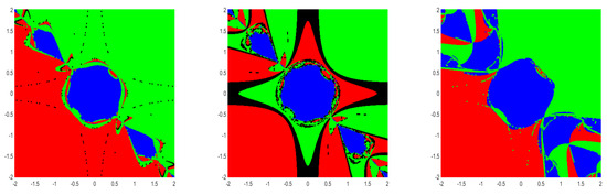
Figure 2.
BA for method (5) for the choices , and (left→ right) for Example 6.
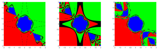
Figure 3.
BA for method (5) for the choices , and (left→ right) for Example 6.
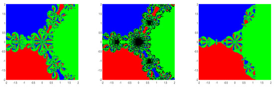
Figure 4.
BA for method (5) for the choices , and (left→ right) for Example 7.
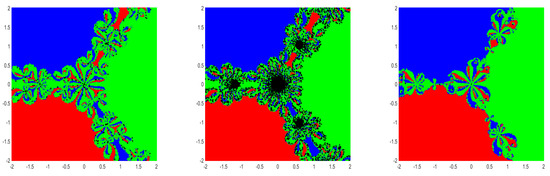
Figure 5.
BA for method (5) for the choices , and (left→ right) for Example 7.
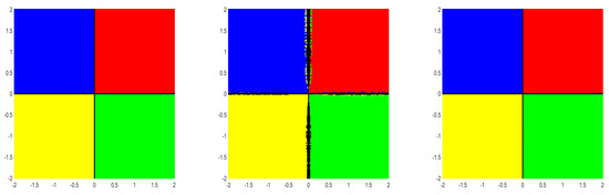
Figure 6.
BA for method (5) for the choices , and (left→ right) for Example 8.
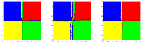
Figure 7.
BA for method (5) for the choices , and (left→ right) for Example 8.
7. Conclusions
We proved the OC of methods (3) and (5) using assumptions only on the first three derivatives of function Ş. We presented the semilocal convergence, and also we used our semilocal analysis to avoid using any assumptions on to prove the local convergence. All these analyses were performed in a more general Banach-space setting. Computable error bounds and uniqueness results are provided. The analysis improves the class of functions to which the methods are applicable. Moreover, it updates the class of methods itself by relaxing the assumptions on the weight function. We presented numerical examples, comparison studies, and dynamics of methods (3) and (5).
Author Contributions
Conceptualization, S.G., A.K., I.K.A. and J.P.; methodology, S.G., A.K., I.K.A. and J.P.; software, S.G., A.K., I.K.A. and J.P.; validation, S.G., A.K., I.K.A. and J.P.; formal analysis, S.G., A.K., I.K.A. and J.P.; investigation, S.G., A.K., I.K.A. and J.P.; resources, S.G., A.K., I.K.A. and J.P.; data curation, S.G., A.K., I.K.A. and J.P.; writing—original draft preparation, S.G., A.K., I.K.A. and J.P.; writing—review and editing, S.G., A.K., I.K.A. and J.P.; visualization, S.G., A.K., I.K.A. and J.P.; supervision, S.G., A.K., I.K.A. and J.P.; project administration, S.G., A.K., I.K.A. and J.P.; funding acquisition, S.G., A.K., I.K.A. and J.P. All authors have read and agreed to the published version of the manuscript.
Funding
This research received no external funding.
Data Availability Statement
Data are contained within the article.
Conflicts of Interest
The authors declare no conflicts of interest.
References
- Moré, J.J. A Collection of Nonlinear Model Problems; Technical Report; Argonne National Lab.: Lemont, IL, USA, 1989. [Google Scholar]
- Lin, Y.; Bao, L.; Jia, X. Convergence analysis of a variant of the Newton method for solving nonlinear equations. Comput. Math. Appl. 2010, 59, 2121–2127. [Google Scholar] [CrossRef]
- Awawdeh, F. On new iterative method for solving systems of nonlinear equations. Numer. Algorithms 2010, 54, 395–409. [Google Scholar] [CrossRef]
- Khlopov, M. Primordial Black Hole Messenger of Dark Universe. Symmetry 2024, 16, 1487. [Google Scholar] [CrossRef]
- Kang, S.; Lee, H. Probabilistic Multi-Robot Task Scheduling for the Antarctic Environments with Crevasses. Symmetry 2024, 16, 1229. [Google Scholar] [CrossRef]
- Bouzeffour, F. Supersymmetric Quesne-Dunkl Quantum Mechanics on Radial Lines. Symmetry 2024, 16, 1508. [Google Scholar] [CrossRef]
- Regmi, S.; Argyros, I.K.; George, S.; Argyros, C.I. Extended Convergence of Three Step Iterative Methods for Solving Equations in Banach Space with Applications. Symmetry 2022, 14, 1484. [Google Scholar] [CrossRef]
- Remesh, K.; Argyros, I.K.; Saeed K, M.; George, S.; Padikkal, J. Extending the applicability of Cordero type iterative method. Symmetry 2022, 14, 2495. [Google Scholar] [CrossRef]
- Artidiello, S.; Cordero, A.; Torregrosa, J.R.; Vassileva, M.P. Multidimensional generalization of iterative methods for solving nonlinear problems by means of weight-function procedure. Appl. Math. Comput. 2015, 268, 1064–1071. [Google Scholar] [CrossRef][Green Version]
- Balaji, G.V.; Seader, J.D. Application of interval Newton’s method to chemical engineering problems. Reliab. Comput. 1995, 1, 215–223. [Google Scholar] [CrossRef]
- Cordero, A.; Hueso, J.L.; Martínez, E.; Torregrosa, J.R. A modified Newton-Jarratt’s composition. Numer. Algorithms 2010, 55, 87–99. [Google Scholar] [CrossRef]
- Cordero, A.; Maimó, J.G.; Torregrosa, J.R.; Vassileva, M.P. Solving nonlinear problems by Ostrowski–Chun type parametric families. J. Math. Chem. 2015, 53, 430–449. [Google Scholar] [CrossRef]
- Constantinides, A.; Mostoufi, N. Numerical Methods for Chemical Engineers with MATLAB Applications with Cdrom; Prentice Hall PTR: London, UK, 1999. [Google Scholar]
- Chun, C.; Ham, Y. Some sixth-order variants of Ostrowski root-finding methods. Appl. Math. Comput. 2007, 193, 389–394. [Google Scholar] [CrossRef]
- Sharma, J.R.; Arora, H. Efficient Jarratt-like methods for solving systems of nonlinear equations. Calcolo 2014, 51, 193–210. [Google Scholar] [CrossRef]
- Soleymani, F. Regarding the accuracy of optimal eighth-order methods. Math. Comput. Model. 2011, 53, 1351–1357. [Google Scholar] [CrossRef]
- Ortega, J.M.; Rheinboldt, W.C. Iterative Solution of Nonlinear Equations in Several Variables; SIAM: Montréal, QC, Canada, 2000. [Google Scholar]
- Cordero, A.; Torregrosa, J.R. Variants of Newton’s method for functions of several variables. Appl. Math. Comput. 2006, 183, 199–208. [Google Scholar] [CrossRef]
- Cordero, A.; Torregrosa, J.R. Variants of Newton’s method using fifth-order quadrature formulas. Appl. Math. Comput. 2007, 190, 686–698. [Google Scholar] [CrossRef]
- Collatz, L. Functional Analysis and Numerical Mathematics; Academic Press: New York, NY, USA, 1966. [Google Scholar]
- Alzahrani, A.K.H.; Behl, R.; Alshomrani, A.S. Some higher-order iteration functions for solving nonlinear models. Appl. Math. Comput. 2018, 334, 80–93. [Google Scholar] [CrossRef]
- Argyros, I.K.; Argyros, G.I.; Regmi, S.; George, S. Contemporary Algorithms: Theory and Applications: Vol 4; Nova Science Publishers: New York, NY, USA, 2024. [Google Scholar]
- Amat, S.; Busquier, S.; Grau, À.; Grau-Sánchez, M. Maximum efficiency for a family of Newton-like methods with frozen derivatives and some applications. Appl. Math. Comput. 2013, 219, 7954–7963. [Google Scholar] [CrossRef]
- Grau-Sánchez, M.; Grau, À.; Noguera, M. On the computational efficiency index and some iterative methods for solving systems of nonlinear equations. J. Comput. Appl. Math. 2011, 236, 1259–1266. [Google Scholar] [CrossRef]
- Ostrowski, A.M. Iterative Solution of Nonlinear Equations in Several Variables; Academic Press: New York, NY, USA, 1970. [Google Scholar]
- Argyros, I.K. The Theory and Applications of Iteration Methods; CRC Press: Boca Raton, FL, USA, 2022. [Google Scholar]
- Behl, R.; Kansal, M.; Salimi, M. Modified King’s Family for Multiple Zeros of Scalar Nonlinear Functions. Mathematics 2020, 8, 827. [Google Scholar] [CrossRef]
- Noor, M.A.; Waseem, M. Some iterative methods for solving a system of nonlinear equations. Comput. Math. Appl. 2009, 57, 101–106. [Google Scholar] [CrossRef]
- Amat, S.; Busquier, S.; Plaza, S. Review of some iterative root–finding methods from a dynamical point of view. Sci. Ser. A Math. Sci. 2004, 10, 3–35. [Google Scholar]
Disclaimer/Publisher’s Note: The statements, opinions and data contained in all publications are solely those of the individual author(s) and contributor(s) and not of MDPI and/or the editor(s). MDPI and/or the editor(s) disclaim responsibility for any injury to people or property resulting from any ideas, methods, instructions or products referred to in the content. |
© 2024 by the authors. Licensee MDPI, Basel, Switzerland. This article is an open access article distributed under the terms and conditions of the Creative Commons Attribution (CC BY) license (https://creativecommons.org/licenses/by/4.0/).