Symmetries of Bernstein Polynomial Differentiation Matrices and Applications to Initial Value Problems

Abstract

In this study, we discuss the symmetries underlying Bernstein polynomial differentiation matrices, as they are used in the collocation method approach to approximate solutions of initial and boundary value problems. The symmetries are brought into connection with those of the Chebyshev pseudospectral method (Chebyshev polynomial differentiation matrices). The treatment discussed here enables a faster and more accurate generation of differentiation matrices. The results are applied in numerical solutions of several initial value problems for the partial differential equation of convection–diffusion reaction type. The method described herein demonstrates the combination of advanced numerical techniques like polynomial interpolation, stability-preserving timestepping, and transformation methods to solve a challenging nonlinear PDE efficiently. The use of Bernstein polynomials offers a high degree of accuracy for spatial discretization, and the CGL nodes improve the stability of the polynomial approximation. This analysis shows that exploiting symmetry in the differentiation matrices, combined with the wise choice of collocation nodes (CGL), leads to both accurate and efficient numerical methods for solving PDEs and accuracy that approach pseudospectral methods that use well-known orthogonal polynomials such as Chebyshev polynomials.

1. Introduction

Spectral methods [1,2,3] are well-established methods for the solution of partial differential equations, mostly known for their superior accuracy. Spectral methods come in a few varieties, such as Galerkin, collocation, and Tau. The difference between them is how one forms the discrete set of equations; from the perspective of the more general framework of weighted residual methods, where the different formulations can be systematized; or based on whether one solves for expansion coefficients or nodal values. Another difference comes from the functions used to approximate the unknown solution. Trigonometric series are used for periodic problems, leading to the so-called Fourier methods [2]. The alternatives are polynomial spectral methods [3], which use special functions in the form of orthogonal polynomials stemming from the singular Sturm–Liouville problem, leading to Jacobi, Chebyshev, and Legendre spectral methods. More details on the theoretical foundations and implementation details of spectral methods can be found in [4,5].

There has been a strong motivation to experiment in forming similar solution methods using other known special functions and polynomials, orthogonal or not. These motivations are specific computational domains: semi-unbounded, cylindrical, spherical, etc., or some other technical or historical reasons.

When it comes to the use of Bernstein polynomials, the roots may be described as historical, as they were employed in one of the initial proofs of the Stone–Weierstrass theorem [6]. Their practical use, other than proving Weierstrass theorem, was somewhat discouraged, and this is often repeated as a fact in numerical analysis textbooks, e.g., ref. [7]. We only partially agree with this point of view since our own work and the works of other researchers show favorable characteristics for certain types of problems and with small and particular modifications. As a footnote, a similar view is found for Lagrange interpolation, for which it is often repeated that it is unstable for higher-order polynomials, while it is pointed out by, e.g., Berrut and Trefethen that this is only partially true—once the non-equidistant set of nodes is used together with the barycentric form of interpolation formula, the said problems are alleviated [8].

Several studies use Bernstein polynomials for numerical solutions of ODEs and PDEs. In [9], the authors used a modified Bernstein polynomial basis within the Galerkin method for highly accurate solutions of one-dimensional boundary value problems. A numerical solution of the KdV–Burgers equation using Bernstein polynomials as trial functions in the Galerkin method is presented in [10]. An approximate method based on Bernstein polynomials for the direct solution of third-order ODEs applied to fluid-flow equations is shown in [11]. A collocation method [12,13] based on Bernstein polynomials for two-dimensional elliptic boundary value problems is introduced in [14]. The Bernstein collocation method for a class of Sturm–Liouville problems is shown in [15]. The solution of high-even-order differential equations using the Bernstein Galerkin and Bernstein Petrov–Galerkin methods is presented in [16]. The Bernstein Ritz–Galerkin method is used in [17] for the solution of the initial–boundary value problem for the wave equation. Recently, the applicability of Bernstein polynomials has been extended to fractional diffusion equations in [18].

Differentiation matrices are one of the straightforward methods for the implementation of spectral methods, especially when the programming language used for implementation readily supports the use of these structures, as is the case with Python or MATLAB. Regarding the implementation, the works of Weideman and Reddy [19] and Trefethen [20] have shown how the use of differentiation matrices produces spectral algorithms of elegant form, especially when used in MATLAB, where the idea of manipulating matrix and vector objects is central and particularly efficient. Explicitly defining differentiation matrices can be useful in studying the stability of pseudospectral methods applied to time-dependent problems for partial differential equations [20,21,22]. The use of differentiation matrices presents a favorable alternative, even when the fast transform method is available for differentiation, under certain limitations, which are described in [4]. Finally, the use of differentiation matrices enables the easy generalization of spectral methods to higher dimensions through the use of the Kronecker product [14,20].

In this study, we use the familiar idea of a differentiation matrix, a well-established notion in the world of spectral methods, and apply it to Bernstein polynomials. The novelty of the paper is in recognizing that, under a suitable choice of the collocation points, Bernstein polynomial differentiation matrices possess identical symmetries, as in the case of the Chebyshev spectral method, which makes the numerical efficiency and accuracy improvement methods extensively studied in the Chebyshev case [23,24,25,26] relevant in the case of the Bernstein polynomial collocation method as well. The significance of the study is in establishing a deeper connection between the Chebyshev and Bernstein collocation methods.

In this paper, we are focused on initial value problems for PDEs, using the method of lines, where spatial and temporal discretization are independent. The solution of such problems amounts to applying the differential operator in matrix form at every timestep, and multiple times at each timestep in the case of methods such as Runge–Kutta, which brings about the amplification of errors related to applying the matrix differentiation operator. Under such circumstances, accuracy improvements to the Bernstein polynomial collocation method are important, as they are in the Chebyshev polynomials case. We are interested in classical problems of transport phenomena—diffusion, convection, convection–diffusion, and nonlinear transport problems—which can be transformed to these (e.g., via the Cole–Hopf transformation).

The rest of this paper is structured as follows. In Section 2, we provide preliminary notions regarding the Bernstein polynomials; then, we discuss the differentiation matrices and their symmetry properties for the formulation of the present polynomial collocation method. In Section 3, we present the numerical method for the discretization and solution of PDEs and discuss the stability of the method. In Section 4, we provide several application examples of the proposed method for time-dependent problems of PDEs, where we scrutinize the proposed method in detail. We provide the conclusions in Section 5.

2. Theoretical Background

2.1. Bernstein Polynomials

What we refer to as the Bernstein-basis polynomials of degree n are defined as

$$B_{k,n}\left(x\right)=\left({\displaystyle \genfrac{}{}{0pt}{}{n}{k}}\right)x^k{(1-x)}^{n-k},k=0,1,\dots ,n$$

(1)

where ${\displaystyle \left(\genfrac{}{}{0pt}{}{n}{k}\right)}$ is the binomial coefficient:

$$\left({\displaystyle \genfrac{}{}{0pt}{}{n}{k}}\right)={\displaystyle \frac{n!}{k!(n-k)!}}.$$

The set ${\left\{B_{k,n}\left(x\right)\right\}}_{k=0}^n$ forms a basis for the space of polynomials of degree n defined over the unit interval. The Bernstein polynomial is a linear combination of Bernstein-basis polynomials. The derivative of a Bernstein polynomial $B_{k,n}\left(x\right)$ is given as

$${\displaystyle \frac{d}{dx}}{B}_{k,n}\left(x\right)=n\left[B_{k-1,n-1}\left(x\right)-B_{k,n-1}\left(x\right)\right],$$

(2)

where $B_{k-1,n-1}\left(x\right)$ is zero if $k=0$.

The relevant properties are as follows:

• $B_{i,n}\left(x\right)=0$, if $i<0$ or $i>n$;
• Non-negativity: $B_{i,n}\left(t\right)\ge 0$, $t\in [0,1]$;
• Partition of unity: ${\sum }_{i=0}^n{B}_i^n\left(t\right)=1$, for $t\in [0,1]$;
• Symmetry: $B_{i,n}\left(t\right)=B_{n-i,n}(1-t)$;
• Recursion: $B_{i,n}\left(t\right)=(1-t)B_{i,n-1}\left(t\right)+t{B}_{i-1,n-1}\left(t\right)$;
• Interval end conditions: $B_{i,n}\left(0\right)={\delta }_{i,0}$ and $B_{i,n}\left(1\right)={\delta }_{i,n}$, where ${\delta }_{i,j}=\left\{\begin{array}{cc}\hfill 1\hfill & \hfill \mathrm{if}i=j\hfill \\ \hfill 0\hfill & \hfill \mathrm{if}i\ne j\hfill \end{array}\right.$;
• Linear precision: ${\sum }_{i=0}^n{\displaystyle \frac{i}{n}}{B}_i^n\left(t\right)=t$;
• Single maximum: For every $B_{i,n}\left(t\right),i=1,2,\dots n$, there is one maximum at $t=i/n$.

Bernstein polynomials can be defined over arbitrary real-line segments. The Bernstein polynomials of n-th degree that form a complete basis over $[a,b]$ are defined by

$$B_{i,n}^{[a,b]}\left(x\right)=\left({\displaystyle \genfrac{}{}{0pt}{}{n}{i}}\right){\displaystyle \frac{{(x-a)}^i{(b-x)}^{n-i}}{{(b-a)}^n}},i=0,1,\dots ,n.$$

(3)

The first derivative is obtained as

$${\displaystyle \frac{d}{dx}}{B}_{k,n}^{[a,b]}\left(x\right)={\displaystyle \frac{n}{b-a}}\left[B_{k-1,n-1}^{[a,b]}\left(x\right)-B_{k,n-1}^{[a,b]}\left(x\right)\right].$$

(4)

The relevant properties listed above are maintained in essence, although adjusted for the domain of definition.

2.2. Differentiation Matrices and Their Symmetries

The differentiation matrix represents the discrete approximation of the derivative operator in the polynomial basis. When applied to a vector of function values, it provides an approximation to the derivative of the function at the corresponding points. In this way, differentiation matrices are an efficient approach to implement spectral methods [20].

The differentiation matrix for Bernstein polynomials can be constructed by considering the derivative relationship between the Bernstein polynomials (Equation (2)). Using the above definition and a standard set of equidistant collocation points leads to inaccuracy for the practical solution of PDEs when using the polynomial collocation method formulated in terms of differentiation matrices. This situation can be remedied by introducing several useful modifications. The generalization leads to an explicit definition of the arbitrary integer-order derivative of the Bernstein polynomial defined over an arbitrary real segment, which can be used for the explicit definition of differentiation matrix elements for an arbitrary set of collocation points.

Theorem 1 

([16]). Explicit formula for the p-th-order derivative of Bernstein polynomials defined over unit segment is given as

$$D^{\left(p\right)}{B}_{i,n}\left(x\right)={\displaystyle \frac{n!}{(n-p!)}}\sum _{k=max(0,i+p-n)}^{min(i,p)}{(-1)}^{(k+p)}\left({\displaystyle \genfrac{}{}{0pt}{}{p}{k}}\right)B_{i-k,n-p}\left(x\right).$$

(5)

As shown in Equation (3), Bernstein polynomials can be defined over a general interval, and there exists the explicit formula for the arbitrary-order differentiation of Bernstein polynomial-basis functions defined over such an interval. Generalizing the result of Doha et al. [16], we give an explicit formula for the calculation of arbitrary-order derivatives of Bernstein-basis functions of any order, defined over an arbitrary interval (see also [14]).

Lemma 1. 

Let $B_{i,n}^{[a,b]}\left(x\right)$ define the i-$th$ Bernstein polynomial defined over $[a,b]$ of n-th order, at point x, where $x\in [a,b]$, and $i=0,\dots ,n$. Then, the derivative of order p of such a basis function can be expressed as

$$D^{\left(p\right)}{B}_{i,n}^{[a,b]}\left(x\right)={\displaystyle \frac{n!}{(n-p!){(b-a)}^p}}\sum _{k=max(0,i+p-n)}^{min(i,p)}{(-1)}^{(k+p)}\left({\displaystyle \genfrac{}{}{0pt}{}{p}{k}}\right)B_{i-k,n-p}^{[a,b]}\left(x\right).$$

(6)

Proof. 

The proof closely follows the proof by the induction of Theorem 1 in [16].    □

Using this expression, one can construct differentiation matrices for Bernstein polynomial-basis functions, defined over an arbitrary set of collocation points $\left\{x_i\right\}$. The differentiation matrices are produced in a straightforward way, given a set of collocation points of a pseudospectral method $D_{i,j}$, the entry of the differentiation matrix is obtained by the evaluation of the j-th basis function at the i-th collocation point [20].

In the present study (as in [14]), the differentiation matrix D is constructed based on the Chebyshev–Gauss–Lobatto (CGL) nodes:

$$x_i=cos\left({\displaystyle \frac{\pi i}{n}}\right)\mathrm{for}i=0,1,\dots ,n.$$

(7)

While interpolation using Bernstein polynomials at equidistant nodes has a meaning—the coefficients of Bernstein polynomial expansion have the same value as samples at equidistant points of the function that the Bernstein interpolant approximates—we have chosen CGL nodes, which known for producing better accuracy and stability properties of the interpolant.

Using expressions given by Equations (3), (6) and (7), the main building blocks of the present Bernstein polynomial collocation algorithm are defined. In an example implementation of the differentiation matrices up to order four, Bernstein-basis function matrices B and nodal points are produced by a simple Python function (see Appendix A).

2.3. Symmetries of Differentiation Matrices

To improve the performance of the implementation of Chebyshev spectral methods, various authors [23,24,25,26] observed and systematically employed the symmetry properties of the differentiation matrices to produce algorithms with increased efficiency compared to the baseline case.

In polynomial collocation methods (e.g., Bernstein or Chebyshev), differentiation matrices approximate the derivatives of the solution at collocation points. These matrices, denoted $D=\left[D_{i,j}\right],i,j=0,1,\dots ,n$ for the first derivative and ${\mathbf{D}}^{\mathbf{2}}$ for the second derivative, are computed by evaluating the derivative of each basis function at the chosen set of collocation points, e.g., $D_{ij}^{\left(p\right)}=D^{\left(p\right)}{B}_{i,n}\left(x_j\right),i,j=0,1,\dots ,n$, from (6).

Here, we demonstrate that, if CGL points are chosen as collocation points, the same set of symmetry conditions applies in the case of Bernstein polynomials as it does in the Chebyshev case, which can be used to our advantage.

Theorem 2. 

For Bernstein polynomial differentiation matrices defined by Equation (6) and a symmetric distribution of collocation nodes, the following symmetry properties hold:

• Odd-order differentiation matrices are centro-antisymmetric:

  $$D_{i,j}^{\left(p\right)}=-D_{n-i,n-j}^{\left(p\right)},i,j=0,\dots ,n,p-odd$$
• Even-order differentiation matrices are centro-symmetric:

  $$D_{i,j}^{\left(p\right)}=D_{n-i,n-j}^{\left(p\right)},i,j=0,\dots ,n,p-even$$

Proof. 

Let’s start by moving the origin of the coordinate system to the midpoint of the real line segment $[a,b]$. The support of the Bernstein polynomials then becomes $x\in [-c,c],c=(b-a)/2$. Next, we create new piecewise functions by using pairs of Bernstein polynomials $B_{i,n}^{[-c,c]}\left(x\right)$ and $B_{n-i,n}^{[-c,c]}\left(x\right)$, $i=0,1,\dots ,⌊(n+1/2)⌋$, which figure in the symmetry relation of Bernstein polynomials as follows (we leave out the $[-c,c]$ superscript):

$$C_i\left(x\right)=\left\{\begin{array}{cc}\hfill B_{i,n}\left(x\right)\hfill & \hfill \mathrm{if}x\in [-c,0),\hfill \\ \hfill B_{n-i,n}\left(x\right)\hfill & \hfill \mathrm{if}x\in [0,c]\hfill \end{array}\right.$$

and

$$C_{n-i}\left(x\right)=\left\{\begin{array}{cc}\hfill B_{n-i,n}\left(x\right)\hfill & \hfill \mathrm{if}x\in [-c,0),\hfill \\ \hfill B_{i,n}\left(x\right)\hfill & \hfill \mathrm{if}x\in [0,c].\hfill \end{array}\right.$$

The Bernstein polynomial $B_{(n+1)/2,n}\left(x\right)$, when n is even, is left as is. Now, the symmetry of Bernstein polynomials becomes a parity property. These new piecewise functions are even functions, with discontinuous first derivative at $x=0$. The derivative of a continuous even function, with discontinuity in the first derivative at $x=0$ is a discontinuous at $x=0$ odd function with continuous first derivative, i.e., $d^p{C}_i(-x)/d{x}^p={(-1)}^p{d}^p{C}_i\left(x\right)/d{x}^p,1\le p\le n$. The symmetry of collocation points leads to the proposed symmetries of differentiation matrices $D_{i,j}^{\left(p\right)}={(-1)}^p{D}_{n-i,n-j}^{\left(p\right)},1\le p\le n$.    □

In this article, after demonstrating the desired symmetry properties for Bernstein polynomial differentiation matrices, they are used for the Bernstein polynomial collocation method.

The flipping trick and negative sum trick are numerical techniques that exploit the inherent symmetries in the differentiation matrices and have previously been used for Chebyshev pseudospectral methods. These tricks lead to improved accuracy and numerical efficiency (by computational savings), particularly when solving initial value problems (IVPs) for partial differential equations.

In the following, the CGL collocation points in (7) are assumed.

2.3.1. Application of Symmetry Properties in Bernstein Polynomials

The flipping trick is a technique used to avoid redundant computations when constructing differentiation matrices for functions that exhibit mirror symmetry about the midpoint of the domain. In both Chebyshev and Bernstein polynomials, the values of the basis functions and their derivatives at the collocation points on one half of the domain are related to the values on the other half through symmetry.

In the algorithm for setting up differentiation matrices, only the differentiation matrices for the first half of the CGL nodes are computed directly. The matrix for the remaining nodes is obtained by flipping (mirroring) the computed values:

$$B[n1:,:]=\mathrm{flipud}\left(\mathrm{fliplr}\right(B[0:n2,:]\left)\right),$$

$$D[n1:,:]=-\mathrm{flipud}\left(\mathrm{fliplr}\right(D[0:n2,:]\left)\right),$$

$$D^{\left(2\right)}[n1:,:]=\mathrm{flipud}\left(\mathrm{fliplr}\left(D^{\left(2\right)}[0:n2,:]\right)\right).$$

Here, ‘flipud’ flips the matrix upside down, and ‘fliplr’ flips it left to right. The negative sign accounts for the change in the derivative direction when flipping. The indices used in array slicing are defined as $n1=⌊(n+1)/2⌋$ and $n2=⌈(n+1)/2⌉$ and cover both even and odd cases of polynomial order n.

The significance of utilizing symmetry in such a way is in accuracy, memory efficiency, and computational efficiency. By exploiting the symmetry of the problem, this method avoids the accumulation of small numerical errors that would occur if both halves were computed separately. Reducing the number of direct computations helps reduce memory consumption, which is particularly important in large-scale PDE problems. The differentiation matrix flipping nearly half the number of computations is needed to construct the differentiation matrices, especially for higher-order polynomials with a large number of collocation points.

Using even–odd decomposition [27] is one additional way of achieving the advantages mentioned above. Let’s consider the derivative evaluated by matrix–vector product ($u_i\equiv u\left(x_i\right)$):

$$u_i^{\prime }=\sum _{j=0}^n{D}_{i,j}{u}_j,i=0,1,\dots ,n.$$

(8)

The vector $u_i$ can be decomposed into two parts:

$$\mathbf{u}=\mathbf{e}+\mathbf{o},$$

(9)

where

$$\begin{array}{c}\hfill e_i=u_i+u_{n-i},\end{array}$$

(10)

$$\begin{array}{cc}\hfill o_i=u_i-u_{n-i},& \hfill i=0,1,\dots ,{\displaystyle \frac{n-1}{2}}.\hfill \end{array}$$

(11)

and $e_{n-j}=e_j,o_{n-j}=-o_j$.

Their derivatives are obtained by

$$e^{\prime }=D_{e}e,$$

$$o^{\prime }=D_{o}o,$$

where

$$\begin{array}{c}\hfill {\left(D_e\right)}_{i,j}={\displaystyle \frac{1}{2}}(D_{i,j}+D_{i,n-j}),\end{array}$$

(12)

$$\begin{array}{cc}\hfill {\left(D_o\right)}_{i,j}={\displaystyle \frac{1}{2}}(D_{i,j}-D_{i,n-j}),& \hfill i,j=0,1,\dots ,{\displaystyle \frac{n-1}{2}}.\hfill \end{array}$$

(13)

Then, the derivative $u^{\prime }\left(x_i\right),i=0,\dots ,n$ is obtained as

$$\begin{array}{c}\hfill u_i^{\prime }=o_i^{\prime }+e_i^{\prime },\end{array}$$

(14)

$$\begin{array}{cc}\hfill u_{n-i}^{\prime }=o_i^{\prime }-e_i^{\prime },& \hfill i=0,1,\dots ,{\displaystyle \frac{n-1}{2}}.\hfill \end{array}$$

(15)

Even–odd decoupling uses almost half as many operations to obtain the approximate derivative relative to the matrix–vector multiplication algorithm ($n^2+n$ compared to $2n^2-n$ operations for the direct matrix–vector product; see [5]).

Next, the accuracy-improving measure of the present method is the “Negative Sum Trick” (NST) [23,24,25]. The negative sum trick ensures that the differentiation matrices sum to zero along their rows, which improves the overall accuracy of the differentiation matrix. For differentiation matrices, each row represents the discrete derivative of a polynomial at a collocation point. The sum of the entries in each row should ideally be zero because the derivative of a constant function is zero everywhere. In practice, due to floating-point errors, this condition may not hold exactly.

For each row i, the sum of the entries must satisfy

$$\sum _{j=0}^n{D}_{ij}=0,i=0,1,\dots ,n.$$

(16)

In the algorithm, this is performed by subtracting the sum of each row of the differentiation matrix from its diagonal element, forcing the rows to sum to zero:

$$D=D-\mathrm{diag}(\sum D,\mathrm{axis}=1),$$

(17)

$$D^{\left(2\right)}=D^{\left(2\right)}-\mathrm{diag}(\sum D^{\left(2\right)},\mathrm{axis}=1)$$

(18)

By enforcing the zero-sum property, the NST reduces the accumulation of floating-point errors in the differentiation process without introducing significant complexity into the algorithm.

For PDE solvers using collocation methods, these optimizations in the accuracy of differentiation matrices translate directly into better accuracy for the numerical solution. This is crucial in long-time integration problems, where small errors can accumulate and lead to large deviations from the true solution.

2.3.2. Forward Test for the Approximate Derivative

The following test provides a comprehensive evaluation of the performance of Bernstein polynomial-based numerical differentiation for a nontrivial test function. The Bernstein differentiation matrix of different polynomial orders is used to approximate the derivatives of the interpolated function at the collocation points. The function being tested is ${\displaystyle f\left(x\right)=\frac{sin\left(8x\right)}{{(x+1.1)}^{3/2}}}$, as tested in [26] for Chebyshev differentiation matrices. First, the Bernstein polynomial expansion coefficients, approximating $f\left(\overline{x}\right),\overline{x}=\left[x_i\right],i=0,1,\dots ,n,$ are computed by solving the system

$$B\beta =f\left(\overline{x}\right),$$

(19)

where B is the Bernstein-basis matrix and $\beta$ are the expansion coefficients. The numerical derivative of the interpolated function is then computed as

$$f_N^{\prime }\left(\overline{x}\right)=D\beta ,$$

(20)

where D is the first-order differentiation matrix for Bernstein polynomials and N indicates the polynomial order used in approximating the function. The maximum absolute error between the numerical derivative $f_N^{\prime }\left(\overline{x}\right)$ and the analytical derivative,

$$\mathrm{error}=max|f_N^{\prime }\left(x_i\right)-f^{\prime }\left(x_i\right)|,i=0,1,\dots ,n,$$

(21)

is used to assess the accuracy of numerical differentiation for different orders of the Bernstein polynomial. In Figure 1 and Figure 2, the maximum error as a function of the Bernstein polynomial order is shown on a logarithmic scale, for the baseline and improved cases, respectively. For the forward problem, the improvement resulting from the introduced modifications in both accuracy and convergence is observed in Figure 2. The plot is typical for the numerical differentiation of smooth functions using spectral methods. At $N=21$, the error reaches the round-off error level and remains at that level for the higher polynomial orders. The accuracy level of the improved Bernstein case can be compared to that of the Chebyshev case (see [26]).

3. The Numerical Solution Method

The Bernstein polynomial differentiation matrices discussed previously are used to implement the Bernstein polynomial collocation method for time-dependent problems of typical transport equations. The method of lines is employed, so the spatial discretization, temporal discretization, and stability are discussed next.

3.1. PDE Discretization by Bernstein Polynomial Collocation Method

The unknown solution $u(x,t)$ is expanded in terms of Bernstein polynomials $B_k^n\left(x\right)$:

$$u(x,t)\approx \sum _{k=0}^n{\beta }_k\left(t\right)B_{k,n}\left(x\right),$$

(22)

where ${\beta }_k\left(t\right)$ are the time-dependent coefficients and $B_{k,n}\left(x\right)$ are the Bernstein-basis polynomials of degree n. The time-varying expansion coefficients ${\beta }_k\left(t\right)$ are the principal unknown.

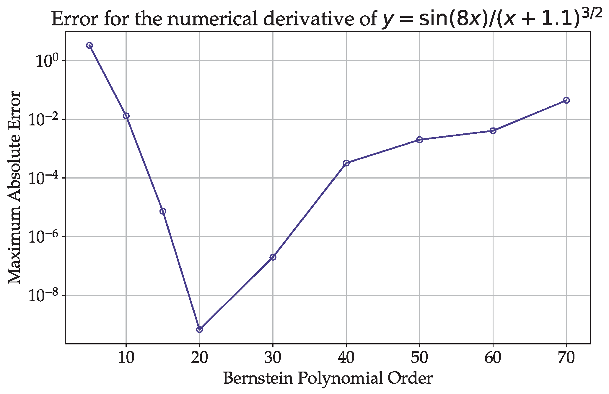
The Bernstein differentiation matrices for the numerical derivative of the first order D, and second order $D^{\left(2\right)}$, are computed using Bernstein polynomials, evaluated at Chebyshev–Gauss–Lobatto (CGL) nodes by leveraging the flipping and negative sum trick (NST) to improve accuracy (Equations (3), (6) and (7) and Algorithm 1). The spatial domain is defined on the segment $[-1,1]$ and transformed to order domains if necessary.

The spatial discretization is described using an example of a constant-coefficient convection–diffusion equation. The special cases are described in greater detail in the numerical examples section.

For the constant-coefficient convection–diffusion equation

$${\displaystyle \frac{\partial u}{\partial t}}+c{\displaystyle \frac{\partial u}{\partial x}}=\gamma {\displaystyle \frac{{\partial }^{2}u}{\partial x^2}},$$

(23)

the semi-discrete form is given by

$${\displaystyle \frac{d{\beta }_k}{dt}}=\sum _{j=0}^n{A}_{kj}{\beta }_j,k=0,1,\dots ,n.$$

(24)

where the Bernstein polynomial expansion coefficients $\beta =\left[{\beta }_j\right],j=0,1,\dots n$ are the unknowns.

The discrete spatial derivatives operator matrix $A=\left[A_{kj}\right],k,j=0,1,\dots n$ is obtained after substituting the approximate derivatives using Bernstein polynomial differentiation matrices ${\displaystyle \frac{\partial u}{\partial x}=D\beta }$, ${\displaystyle \frac{{\partial }^{2}u}{\partial x^2}=D^{\left(2\right)}\beta }$, and $u=B\beta$ into Equation (23). Then,

$${\displaystyle \frac{d\left(B\beta \right)}{dt}}=\left(\gamma D^{\left(2\right)}-cD\right)\beta .$$

(25)

From there, it follows that

$$A=\left(\gamma B^{-1}{D}^{\left(2\right)}-c{B}^{-1}D\right),$$

(26)

where $B^{-1}$ is the inverse of the Bernstein-basis matrix. From the approximately constant-coefficient convection–diffusion equation, the special cases of advection and diffusion equations arise as special cases. The advection equation is discretized as

$${\displaystyle \frac{d\beta }{dt}}=A\beta ,$$

(27)

where the system matrix is constructed as

$$A=-c{B}^{-1}D.$$

(28)

The numerical setup for the diffusion equation proceeds by using the second-order differentiation matrix $D^{\left(2\right)}$ to represent the diffusion term ${\displaystyle \gamma \frac{{\partial }^{2}u}{\partial x^2}}$, and the system matrix A becomes

$$A=\gamma B^{-1}{D}^{\left(2\right)}.$$

(29)

The convection–diffusion equation discretization presented here for the Bernstein polynomial collocation can be compared to Chebyshev pesudospectral discretization [19,20,21], where the system matrix for the convection–diffusion equation takes the form

$$A=-c{D}_{Cheb}+\gamma D_{Cheb}^{\left(2\right)},$$

(30)

for the constant-speed advection equation, it is defined as

$$A=-c{D}_{Cheb}.$$

(31)

and for the diffusion equation, it takes the form

$$A=\gamma D_{Cheb}^{\left(2\right)}.$$

(32)

In Equations (30)–(32), the $D_{Cheb}$, and $D_{Cheb}^{\left(2\right)}$ are the first- and second-order Chebyshev differentiation matrices.

The Chebyshev pseudospectral method is known for its high accuracy and stability and is used later to assess the relative accuracy of the present method.

The numerical solution process is as follows. First, the initial condition for $u(x,0)$ is set. Then, the coefficients $\beta$ of the Bernstein polynomial expansion of unknown solution $u(x,t)$ are computed by solving the linear system $B\beta =u(x,0)$. The Bernstein polynomial expansion coefficients $\beta$ are advanced in time. At the desired timestep, the solution $u(x,t)$ is reconstructed from the Bernstein coefficients. The details of timestepping are discussed next.

3.2. Timestepping

In the present study, explicit timestepping methods are used. Although classical Runge–Kutta of the fourth order has been used elsewhere [21,22,26], in the present study, the Strong Stability-Preserving Runge–Kutta (SSP-RK) integrators are employed. For the explicit SSP-RK time discretizations, a general s-stage method is written (in the Shu–Osher form) as

$$\begin{array}{cc}\hfill u^{\left(0\right)}& \hfill =u^n,\hfill \\ \hfill u^{\left(i\right)}& \hfill =\sum _{k=0}^{i=1}{\alpha }_{ik}{u}^{\left(k\right)}+\Delta t{\beta }_{ik}L\left(u^{\left(k\right)}\right),i=1,2,\dots ,s\hfill \\ \hfill u^{n+1}& \hfill =u^{\left(s\right)}.\hfill \end{array}$$

(33)

Here, the system of ODEs for ${\beta }_k\left(t\right),k=0,1,\dots n$, Equation (24), is evolved in time using the five-stage fourth-order SSP-RK(5,4) method by Spiteri and Ruuth [28]:

$$\begin{array}{c}\hspace{1em}\beta \left(1\right)={\beta }^n+0.391752226571890\Delta tA\left({\beta }^n\right)\hfill \\ \beta \left(2\right)=0.444370493651235{\beta }^n+0.555629506348765\beta \left(1\right)+0.368410593050371\Delta tA\left(\beta \left(1\right)\right)\\ \beta \left(3\right)=0.620101851488403{\beta }^n+0.379898148511597\beta \left(2\right)+0.251891774271694\Delta tA\left(\beta \left(2\right)\right)\\ \beta \left(4\right)=0.178079954393132{\beta }^n+0.821920045606868\beta \left(3\right)+0.544974750228521\Delta tA\left(\beta \left(3\right)\right)\\ {\beta }^{n+1}=0.517231671970585\beta \left(2\right)+0.096059710526147\beta \left(3\right)+0.063692468666290\Delta tA\left(\beta \left(3\right)\right)\\ +0.386708617503268\beta \left(4\right)+0.226007483236906\Delta tA\left(\beta \right(4\left)\right),\hfill \end{array}$$

(34)

which has C = 1.508 (Ceff = 0.302). This method is particularly suited for maintaining stability when solving hyperbolic PDEs.

As we can see, at every stage, the discretized differential operator is applied to a solution vector by a matrix–vector product. The application of differentiation matrix symmetries can be used to our advantage, as previously shown, to reduce the number of operations of the direct matrix–vector product. With a higher polynomial order and number of stages in the Runge–Kutta method, the numerical efficiency improvements increase. For SSP-RK5(4), the factor is 6 $\times timesteps\times (N^2-2N)$.

3.3. Stability of the Numerical Method

According to the linear stability analysis, the numerical scheme is stable if the eigenvalues of the system matrix in Equation (24) scaled by the timestep size $\Delta t\sigma \left(A\right)$ fall within the stability region of the timestepping method in the complex plane.

In the present study, we assess the stability of the Bernstein polynomial collocation method relative to the Chebyshev pseudospectral method to gain better insight into comparative advantages; we summarize the result in Figure 3.

In Figure 3a, the computed eigenvalues of the discrete advection operator for Bernstein collocation in (28) and Chebyshev pseudospectral method defined by (31), adjusted for boundary conditions $\tilde{A}=A[1:n,1:n]$, are plotted side-by-side for polynomial order $n=20$. The timestep size $\Delta t=0.08$ is chosen so that the scaled eigenvalues remain within the stability region of the SSP-RK(5,4) method (solid line). The highly distinguishing feature is that both methods produce identical eigenspectra (to a round-off precision), raising questions surrounding the similarity of matrices.

In Figure 3b, the unscaled eigenspectra of the diffusion operator of both methods, defined by Equations (29) and (32), respectively, accounted for the boundary conditions on both sides so that $\tilde{A}=A[1:n-1,1:n-1]$ are plotted for the same polynomial order $n=20$ and for diffusion coefficient $\gamma =0.022$. The eigenvalues are identical (to a round-off precision) and purely imaginary.

In Figure 3c, the eigenvalues of convection diffusion operators for the Bernstein (23) and Chebyshev (30) collocation methods based on the values of advection velocity $c=3.5$, diffusion coefficient $\gamma =0.022$, and $n=20$ (see Figure 3 in [21]) are shown, showing the same pattern as above.

The matrices considered are not normal, so the eigenvalues provide only a necessary, but not sufficient, condition for stability. To further assess the stability, we show the pseudospectra of the system matrices in Figure 4. The stability criterion involving pseudospectra is more strict (see [20]), requiring that the pseudospectra of a certain level be contained in the stability region. In this representation, we can differentiate the footprint of system matrices of the Chebyshev and Bernstein collocation method. The Chebyshev collocation method requires marginally smaller timesteps to achieve stability based on this criterion.

4. Numerical Examples

4.1. Linear Advection Equation

The example numerically solves the one-dimensional linear advection equation using two different methods: Chebyshev pseudospectral and Bernstein polynomial collocation methods (with and without the use of symmetry-based tricks), using Chebyshev–Gauss–Lobatto (CGL) nodes for both.

The problem is to solve the linear advection equation

$${\displaystyle \frac{\partial u}{\partial t}}+a{\displaystyle \frac{\partial u}{\partial x}}=0,$$

(35)

with $a=1.5$, on a domain $[-1,1]$, subject to Dirichlet boundary conditions. The initial condition is ${\displaystyle u(x,0)=sin\left(2x\right)}$, and the boundary condition is ${\displaystyle u(-1,t)=sin(-2-3t)}$. This problem appears in [1].

The problem is approximately solved using two methods. In the Chebyshev collocation method, the Chebyshev differentiation matrix is constructed at the Chebyshev–Gauss–Lobatto nodes, and the right-hand side operator $A=a{D}_{Cheb}$ approximates the spatial derivative in the advection equation. The solution $u(x,t)$ is approximated as a sum of Chebyshev polynomials, and the timestepping is carried out using the SSP-RK(5,4) method. Given the Chebyshev differentiation matrix D, the advection equation is discretized as

$${\displaystyle \frac{d{u}_i}{dt}}=-a\sum _{j=0}^n{D}_{ij}{u}_j,$$

(36)

where $u_i$ is the value of the solution at node $x_i$, and $D_{ij}$ are the elements of the Chebyshev differentiation matrix.

For the Bernstein method, the solution is expanded as a sum of Bernstein-basis functions:

$$u(x,t)=\sum _{k=0}^n{\beta }_k\left(t\right)B_k\left(x\right),$$

(37)

where $B_k\left(x\right)$ are the Bernstein-basis polynomials and ${\beta }_k\left(t\right)$ are the time-dependent coefficients. The advection equation is then discretized as

$${\displaystyle \frac{d{\beta }_k}{dt}}=-a\sum _{j=0}^n{D}_{kj}{\beta }_j,$$

(38)

where $D_{kj}$ is the differentiation matrix in the Bernstein basis. The matrix $A=a{B}^{-1}D$ is constructed, where B is the matrix mapping the Bernstein coefficients to function values at the Chebyshev–Gauss–Lobatto collocation points. The initial function $u(x,0)$ is projected onto the Bernstein polynomial basis, and the Bernstein polynomials’ coefficients evolve in time. For this approach, two cases are considered: with and without the use of symmetry-based tricks. In both cases, the system is evolved in time using the SSP-RK(5,4) method.

After each timestep, the Dirichlet boundary condition at $x=-1$ is enforced by setting ${\displaystyle u(-1,t)=sin(-2-3t)}$.

The exact solution for this problem is ${\displaystyle u_{\mathrm{exact}}(x,t)=sin(2x-3t)}$. The maximum absolute error is computed as the difference between the numerical and exact solutions at the final time.

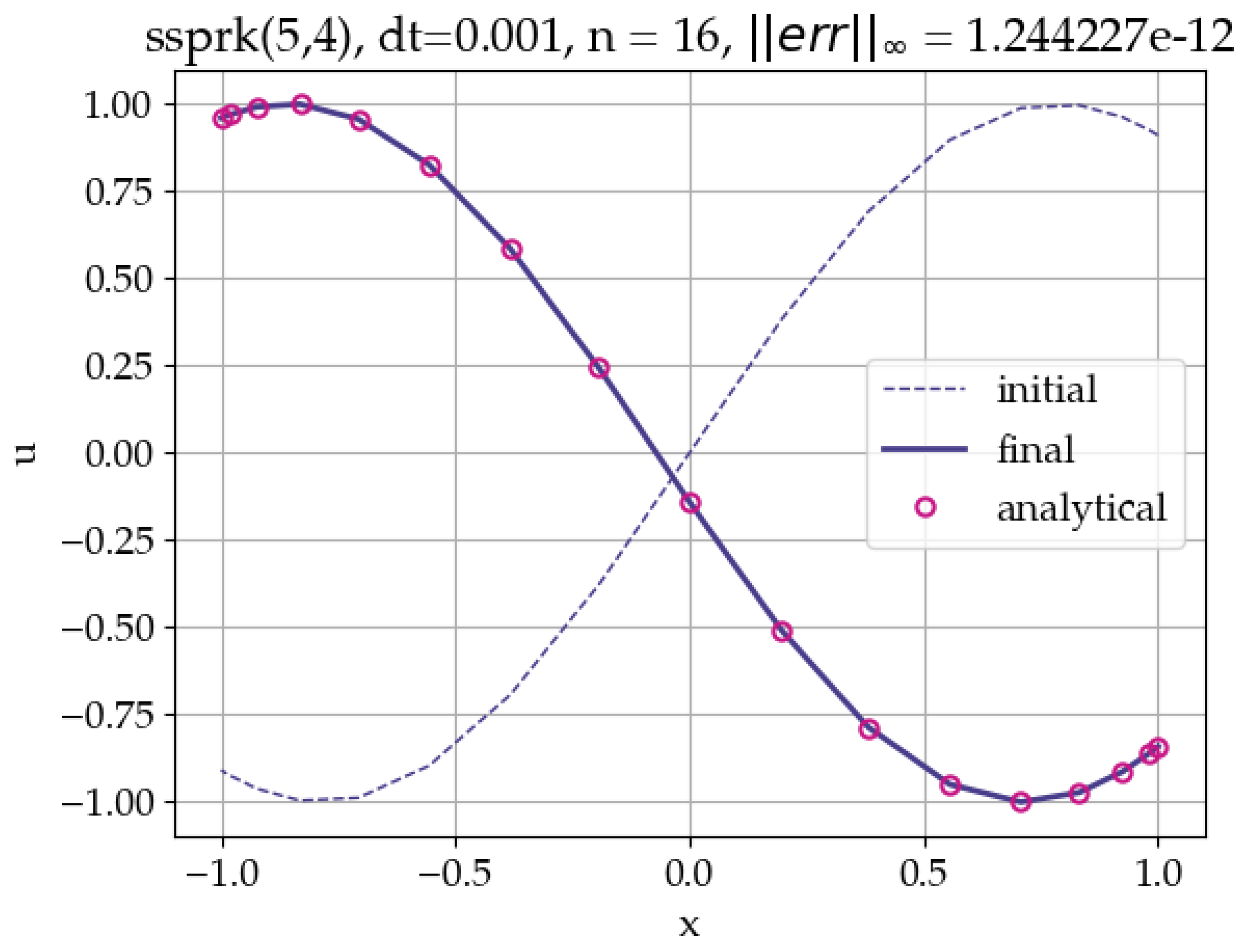
In Figure 5, the representative numerical solution using the Bernstein polynomial collocation, for $n=16$ and timestep size $dt=0.001$, is shown. The figure shows initial, final numerical, and analytical solutions. The advected profile is smooth, which explains the spectral accuracy.

Figure 6 compares the accuracy of the Chebyshev and Bernstein polynomial methods (with and without the symmetry modifications) for solving the linear advection equation. It shows the maximum absolute error between the numerical and exact solutions for various polynomial orders, plotting the error on a log scale to evaluate the performance of each method. High accuracy and spectral convergence is seen for both Chebyshev and Bernstein method. Since the same timestep size is used for all polynomial orders ($dt=1\times {10}^{-5}$), the difference is visible for higher n, due to the loss of stability.

The tabular representation of the convergence of the maximum absolute error is given in

Table 1. Maximum absolute error convergence relative to polynomial order N for three methods.

N	Chebyshev Polynomial	Bernstein Polynomial	Bernstein with Symmetry
8	$2.9297\times {10}^{-5}$	$2.9297\times {10}^{-5}$	$2.9297\times {10}^{-5}$
10	$2.6254\times {10}^{-7}$	$2.6254\times {10}^{-7}$	$2.6254\times {10}^{-7}$
12	$1.7967\times {10}^{-9}$	$1.7967\times {10}^{-9}$	$1.7966\times {10}^{-9}$
14	$8.8787\times {10}^{-11}$	$8.9011\times {10}^{-11}$	$8.9153\times {10}^{-11}$
16	$9.4951\times {10}^{-11}$	$9.6282\times {10}^{-11}$	$9.4638\times {10}^{-11}$
17	$9.4393\times {10}^{-11}$	$9.4028\times {10}^{-11}$	$9.2728\times {10}^{-11}$
18	$9.4254\times {10}^{-11}$	$9.4866\times {10}^{-11}$	$9.3891\times {10}^{-11}$
19	$9.4898\times {10}^{-11}$	$9.6924\times {10}^{-11}$	$9.6055\times {10}^{-11}$
20	$9.4683\times {10}^{-11}$	$8.8217\times {10}^{-11}$	$9.7988\times {10}^{-11}$
21	$9.4234\times {10}^{-11}$	$9.0184\times {10}^{-11}$	$8.2505\times {10}^{-11}$
22	$9.4890\times {10}^{-11}$	$7.7193\times {10}^{-11}$	$7.9375\times {10}^{-11}$
23	$9.4842\times {10}^{-11}$	$1.2173\times {10}^{-10}$	$1.8022\times {10}^{-10}$
24	$9.4242\times {10}^{-11}$	$1.4185\times {10}^{-10}$	$1.3264\times {10}^{-10}$

, to better assess the difference of the three approaches. We see that, unlike the forward problem, the application of symmetries to Bernstein polynomial differentiation matrices produces only very small accuracy improvements. This corroborates similar findings for the Chebyshev case, found in [26].

4.2. Spatially Variable-Coefficient Advection Equation

The problem solved here is used for the finer detail assessment of the Bernstein polynomial collocation method and its improvements via symmetry modifications of differentiation matrices. It was used to test the accuracy improvements for differentiation matrices in the Chebyshev pseudospectral method in [26]. The initial value problem for the variable-coefficient advection equation is given as

$$\begin{array}{cc}\hfill u_t+x{u}_x& \hfill =0,-1\le x\le 1,0<t\le T,\hfill \end{array}$$

(39)

$$\begin{array}{cc}\hfill u(x,0)& \hfill =f\left(x\right),-1\le x\le 1,\hfill \end{array}$$

(40)

where the initial condition is set to ${\displaystyle f\left(x\right)={cos}^2\left(\frac{\pi x}{2}\right)}$, and the exact solution is ${\displaystyle u(x,t)=f\left(xexp(-t)\right)}$. The boundary conditions are not required. Problem (39) is advanced in time using SSP Runge–Kutta 5(4) (the fourth-order Runge–Kutta is used in [26]). The advection equation is discretized as

$${\displaystyle \frac{d\beta }{dt}}=A\beta .$$

(41)

To handle the non-uniform advection coefficient, the matrix A is constructed as

$$A=-B^{-1}\left(\mathbf{x}D\right),$$

(42)

where $B^{-1}$ is the inverse of the Bernstein-basis matrix, D is the Bernstein polynomial differentiation matrix, and $\mathbf{x}$ is a diagonal matrix with the CGL nodes $\left\{x_i\right\}$ on the diagonal.

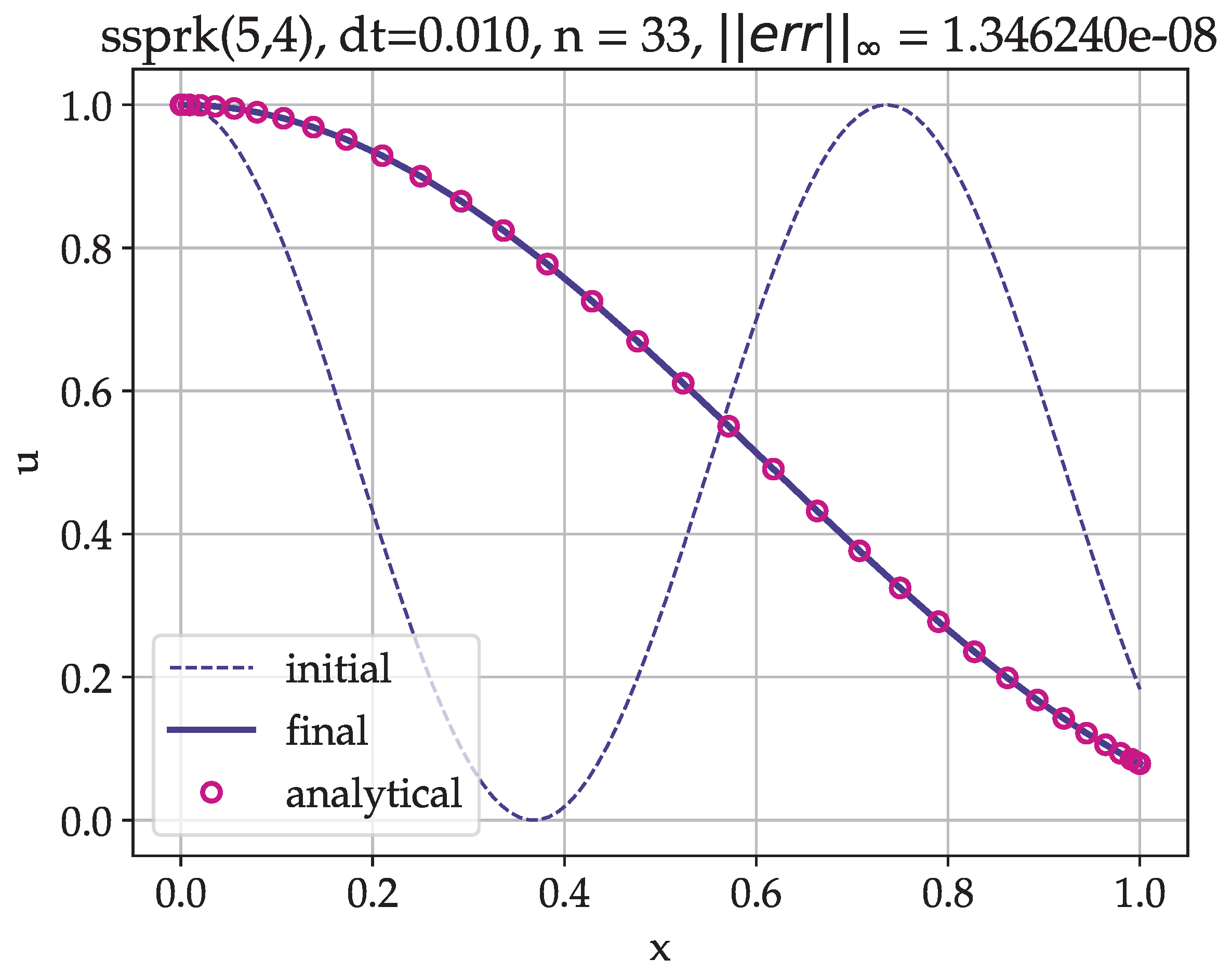
In Figure 7, the representative solution using polynomial order $n=33$ and timestep size $dt=0.01$, together with the initial and analytical solutions, is shown.

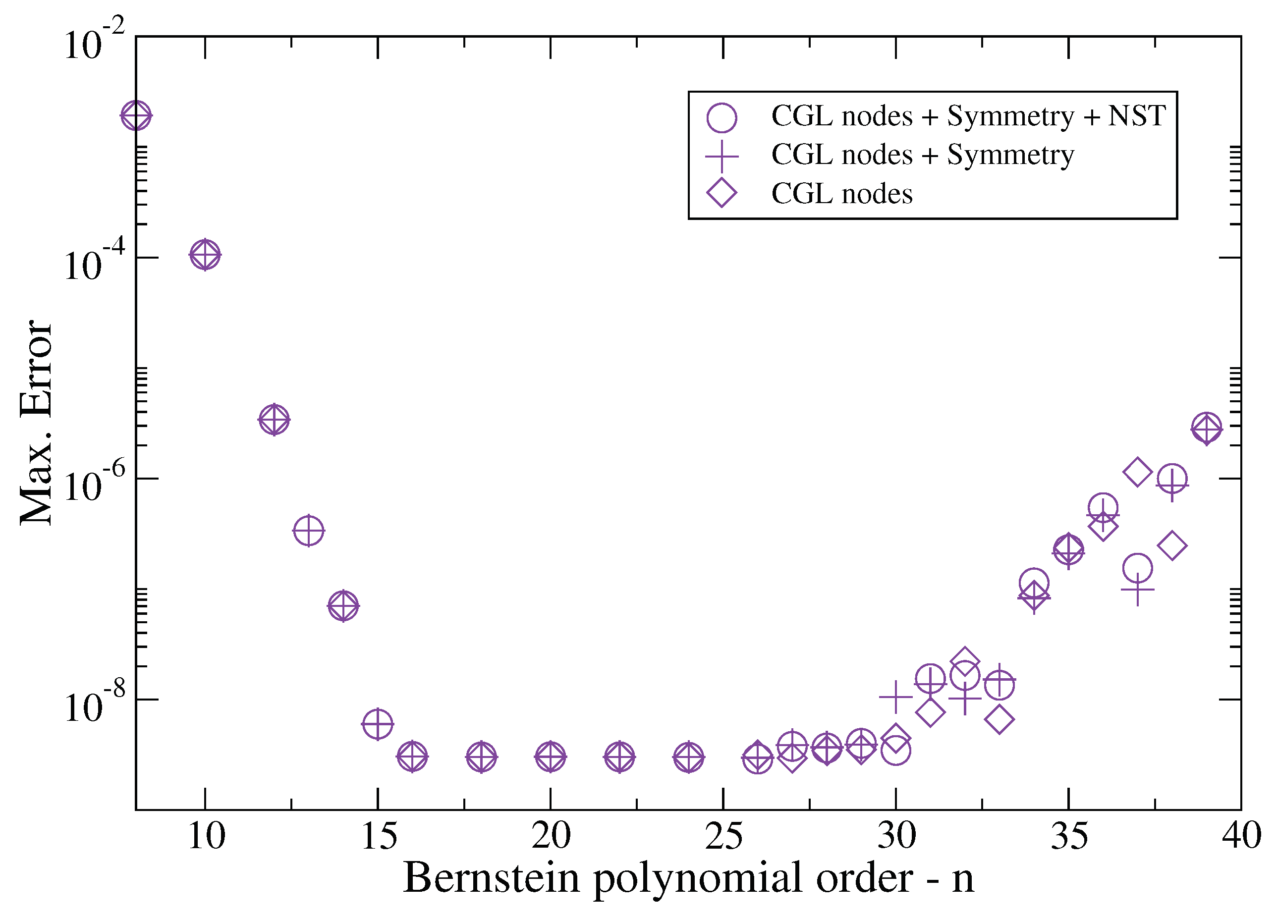
To assess the accuracy improvement of the proposed method, we compare the numerical and analytical solution by plotting the error as a function of polynomial order in Figure 8.

4.3. Nonlinear Convection–Diffusion Equation via Cole–Hopf Transformation

In this example, we consider the nonlinear one-dimensional convection-diffusion equation,

$${\displaystyle \frac{\partial u}{\partial t}}+u{u}_x=\mu u_{xx},$$

(43)

with initial Dirichlet boundary conditions given as

$$u(x,0)=f\left(x\right),0\le x\le 1,$$

(44)

$$u(0,t)=\alpha \left(t\right),u(1,t)=\beta \left(t\right),t\ge 0.$$

(45)

This nonlinear partial differential equation is challenging to solve directly due to the nonlinearity in the convection term. However, using the advantage of the Cole–Hopf transformation, this equation can be linearized; see [29]. Using the Cole–Hopf transformation,

$$u(x,t)=-2\mu {\displaystyle \frac{w_x(x,t)}{w(x,t)}},$$

(46)

in Equation (43), the original equation becomes a heat equation of the following form:

$${\displaystyle \frac{\partial w}{\partial t}}=\mu w_{xx},0\le x\le 1,t\ge 0.$$

(47)

The initial and boundary conditions are consistently transformed to produce the following ones:

$$w(x,0)=exp\left(-{\int }_0^x{\displaystyle \frac{f\left(s\right)}{2\mu }}ds\right),0\le x\le 1,$$

(48)

$$2\mu w_x(0,t)+\alpha \left(t\right)w(0,t)=0,t\ge 0,$$

(49)

$$2\mu w_x(1,t)+\beta \left(t\right)w(1,t)=0,t\ge 0,$$

(50)

After solving the heat equation by advancing the diffusion equation in time and obtaining the solution for $w(x,t)$, we apply the inverse Cole–Hopf transform, Equation (46), to produce the solution $u(x,t)$ to the original nonlinear convection–diffusion problem.

We validate the Bernstein polynomial collocation with symmetry properties applied to differentiation matrices by solving the problem above and compare it against a Chebyshev pseudospectral solution. The problem given by Equations (43)–(45) is solved with $\mu =0.02$, $u(x,0)=sin\left(\pi x\right),0\le x\le 1$, and $\alpha \left(t\right)=\beta \left(t\right)=0$. The Cole–Hopf transformation in (46) produces the following initial and boundary conditions for the new variable:

$$w(x,0)=exp\left({\displaystyle \frac{cos\left(\pi x\right)-1}{2\pi \mu }}\right),0\le x\le 1,$$

(51)

$$w_x(0,t)=w(1,t)=0,t\ge 0,$$

(52)

i.e., the boundary conditions have transformed to zero-Neumann. Physically, the solution starts with a sinusoidal wave that propagates to the right, forming a wavefront that dissipates in time due to the action of viscous dissipation—Figure 9.

In both studied cases, a Strong Stability-Preserving Runge–Kutta, SSP-RK(5,4), for time integration is used. Boundary conditions are explicitly enforced during the time integration.

To gain insight into the relative accuracy of both methods when applied to the same problem, two approaches—the Chebyshev and the Bernstein polynomial methods—are compared by calculating the absolute difference between the final solutions obtained using each method:

$$\mathrm{diff} = |u_{\mathrm{Chebyshev}}\left(x\right)-u_{\mathrm{Bernstein}}\left(x\right)|.$$

(53)

The graph in Figure 10 shows the example absolute difference distribution for the polynomial order $n=30$ and final time $t=2.0$ s. The same timestep size of $dt=1\times {10}^{-4}$ s is used. The magnitude of the differences between the two methods is on the order of ${10}^{-8}$, which indicates an extremely tiny discrepancy. This suggests that both methods are highly accurate and are producing solutions that are nearly identical. The errors of magnitude ${10}^{-8}$ suggest that we are observing the limit of numerical precision rather than any inherent shortcomings in either method. These differences could be attributed to how floating-point arithmetic handles each method’s approach to differentiation and interpolation.

The fluctuations in absolute difference are irregular across the domain $x\in [0,1]$, but the overall magnitude remains small, with no obvious trend. These oscillations in the error could be attributed to differences in how each method approximates the solution at specific points, particularly in regions where boundary conditions might influence the solution.

Table 2. Maximum absolute difference convergence for Bernstein and Chebyshev methods for nonlinear convection–diffusion using Cole–Hopf transformation.

N	Time = 0.5 s	Time = 1.0 s	Time = 1.5 s	Time = 2.0 s
20	$4.6556\times {10}^{-4}$	$6.3691\times {10}^{-4}$	$3.0450\times {10}^{-5}$	$2.5781\times {10}^{-5}$
22	$7.1145\times {10}^{-4}$	$1.2537\times {10}^{-4}$	$3.8916\times {10}^{-5}$	$7.9931\times {10}^{-6}$
24	$2.6036\times {10}^{-4}$	$4.7010\times {10}^{-5}$	$1.7413\times {10}^{-5}$	$6.8082\times {10}^{-7}$
26	$4.3908\times {10}^{-5}$	$5.0630\times {10}^{-5}$	$2.1452\times {10}^{-6}$	$9.5901\times {10}^{-7}$
28	$7.3969\times {10}^{-5}$	$2.0744\times {10}^{-5}$	$1.5481\times {10}^{-6}$	$2.7960\times {10}^{-7}$
30	$4.2066\times {10}^{-5}$	$3.0789\times {10}^{-6}$	$9.6723\times {10}^{-7}$	$2.4258\times {10}^{-8}$
32	$1.4057\times {10}^{-5}$	$2.2765\times {10}^{-6}$	$2.3635\times {10}^{-7}$	$6.8427\times {10}^{-8}$

gives the convergence of the maximum absolute difference between Chebyshev pseudospectral and Bernstein polynomial collocation methods for several values of polynomial order and at four representative time instants.

In general, the Chebyshev method tends to be more computationally efficient due to the use of nodal values of the function. The Bernstein method, in the present form, has negative tradeoff in terms of efficiency when handling boundary conditions as they are applied to nodal values of the function, which requires transformation from expansion coefficient representation to nodal values and back.

The results show that Bernstein polynomial collocation and Chebyshev pseudospectral methods are both highly effective at solving the given problem, with only minor numerical differences arising between the two. The result underscores the robustness of both methods for solving PDEs with high accuracy.

4.4. Non-Stationary Heat Diffusion in One-Dimensional Rod

This example represents a classic case of non-stationary heat conduction in a rod with a time-varying boundary condition at one end and insulation at the other end.

In this example, we solve the unsteady heat diffusion equation in a one-dimensional domain to produce the distribution of the temperature over time given the time-varying boundary condition at one end. The heat-diffusion equation reads

$${\displaystyle \frac{\partial u(x,t)}{\partial t}}=\alpha {\displaystyle \frac{{\partial }^{2}u(x,t)}{\partial x^2}},$$

(54)

where $\alpha$ is the thermal diffusivity coefficient of the material and $u(x,t)$ is an unknown temperature distribution. To parametrize the physical setup, we the use heat constant a, such that the rod has the fixed length given by $l={\displaystyle \frac{a}{\sqrt{\pi }}}$, and the thermal diffusivity is given as $\alpha ={\left(2{\displaystyle \frac{a}{l}}\right)}^2$, i.e., the length of the rod and thermal diffusivity, respectively, are a function of the heat constant a.

The problem simulates the presence of a heat source with oscillating temperature at one end, so, at $x=0$, the Dirichlet boundary condition for the temperature is imposed as $u(0,t)=Asin\left({\displaystyle \frac{a^2}{l^2}}t\right)$. At the other end of the rod, $x=l$, the zero-Neumann boundary condition, is enforced on temperature, implying that there is no heat flux at the end.

The analytical solution representing time-varying temperature distribution in a one-dimensional rod reads as follows:

$$\begin{array}{cc}\hfill u(x,t)=Asin\left({\displaystyle \frac{a^2}{l^2}}t\right)+ \hfill & \hfill \sum _{n=0}^{\infty }{\displaystyle \frac{4{sin}^2\left(\frac{w_n}{2}\right)}{w_n+w_n^5}}sin\left(w_n{\displaystyle \frac{1-x}{2}}\right)·\hfill \\ & \hfill \hspace{1em}\hspace{1em}\left[w_n^{2}exp\left(-w_n\left({\displaystyle \frac{a^2}{l^2}}t\right)\right)-w_n^{2}cos\left({\displaystyle \frac{a^2}{l^2}}t\right)-sin\left({\displaystyle \frac{a^2}{l^2}}t\right)\right],\hfill \end{array}$$

(55)

where $w_n=n/pi+\pi /2$.

The numerical solution is performed using the present method—the Bernstein polynomial collocation method—and using the Chebyshev pseudospectral method. Figure 11 and Figure 12 show the numerical solution using Bernstein polynomials at four characteristic time instances and absolute error distribution for polynomial order $n=24$.

The maximum absolute error convergences for both Bernstein and Chebyshev methods across several polynomial orders and at characteristic instances of time are shown in

Table 3. Maximum absolute error convergence for Bernstein and Chebyshev methods.

a. Bernstein Collocation Method
$\mathit{N}$	Time = 0.25	Time = 0.50	Time = 0.75	Time = 1.00
8	$2.05419\times {10}^{-4}$	$1.73372\times {10}^{-4}$	$3.21948\times {10}^{-4}$	$2.35233\times {10}^{-4}$
12	$2.07676\times {10}^{-4}$	$1.73378\times {10}^{-4}$	$3.24333\times {10}^{-4}$	$2.39406\times {10}^{-4}$
16	$2.096\times {10}^{-4}$	$1.73377\times {10}^{-4}$	$3.26325\times {10}^{-4}$	$2.4143\times {10}^{-4}$
20	$2.08235\times {10}^{-4}$	$1.73388\times {10}^{-4}$	$3.24975\times {10}^{-4}$	$2.395\times {10}^{-4}$
24	$2.07718\times {10}^{-4}$	$1.7316\times {10}^{-4}$	$3.24025\times {10}^{-4}$	$2.39179\times {10}^{-4}$
b. Chebyshev Pseudospectral Method
$\mathit{N}$	Time = 0.25	Time = 0.50	Time = 0.75	Time = 1.00
8	$2.05419\times {10}^{-4}$	$1.73372\times {10}^{-4}$	$3.2194\times {10}^{-4}8$	$2.35233\times {10}^{-4}$
12	$2.07676\times {10}^{-4}$	$1.73378\times {10}^{-4}$	$3.24333\times {10}^{-4}$	$2.39406\times {10}^{-4}$
16	$2.096\times {10}^{-4}$	$1.73378\times {10}^{-4}$	$3.26326\times {10}^{-4}$	$2.4143\times {10}^{-4}$
20	$2.08239\times {10}^{-4}$	$1.73378\times {10}^{-4}$	$3.24967\times {10}^{-4}$	$2.39498\times {10}^{-4}$
24	$2.07676\times {10}^{-4}$	$1.73378\times {10}^{-4}$	$3.24333\times {10}^{-4}$	$2.39406\times {10}^{-4}$

. The number of timesteps is large and most of the error comes from temporal and not spatial discretization, leading to the small difference between these two higher-order methods.

5. Conclusions

The implementation of the polynomial collocation solution method for initial value problems of partial differential equation using Bernstein polynomials defined over arbitrary real-line segments, in collocation points based on Chebyshev–Gauss–Lobatto points, produces differentiation matrices that possess particular symmetry properties, which may be exploited for numerically efficient and accurate computation. In analogy with Chebyshev spectral method differentiation matrices, it is concluded that Bernstein polynomials possess centro-antisymmetric odd-order differentiation matrices and centro-symmetric even-order differentiation matrices. These symmetry properties are used to reduce the number of operations for the generation of differentiation matrices by using ‘flipping’, described originally for Chebyshev differentiation matrices. Also, the opportunity of using efficient matrix–vector products is possible in the presence of these symmetries. Further, round-off errors are reduced in a similar manner as with the Chebyshev case using negative sum trick.

Moreover, important results follow from the formulation of the Bernstein polynomial collocation method on Chebyshev–Gauss–Lobatto collocation points for linear initial value problems. The eigenvalues of the system matrices for the linear constant-coefficient convection–diffusion problem match on all tested polynomial orders of practical interest for the Chebyshev and Bernstein collocation methods described in this article. However, their pseudospectra differ, leading to marginally different stability properties.

This comparison of the Bernstein collocation and Chebyshev pseudospectral approaches validates both methods as highly accurate, with differences negligible for most practical purposes. If the goal is to obtain a reliable solution for a PDE, either method could be used, depending on the specific requirements.