Abstract
This study presents an in-depth analysis of the macroscopic mechanical properties of periodic nanocomposites containing arbitrarily-shaped inclusions, with a particular focus on the effective stiffness and its dependence on microstructural parameters. We employ a complex variable method to address the problem, considering the interface elasticity effect, which may significantly influence the stress distribution and overall stiffness of the nanocomposites. The research reveals that the effective stiffness of the nanocomposites is not only dependent on the volume fraction and shape of the inclusions but also on the interface properties, particularly the interface elasticity parameter. Our findings indicate that an increase in the interfacial elasticity parameter results in a stiffer composite, highlighting the importance of interfacial effects in determining the mechanical behavior of nanocomposites. The study also explores the impact of inclusion size and orientation on the effective stiffness, demonstrating size-dependent phenomena and the influence of orientation angle on the stiffness elements. These insights contribute to a better understanding of the mechanical properties of nanocomposites and provide a foundation for the design of materials with tailored properties for specific engineering applications.
1. Introduction
The advent of nanocomposites, which incorporate nanoscale inclusions as reinforcing elements, has marked a significant leap forward in material science and technology. These advanced materials have been studied in various fields [1,2,3,4,5] such as force-electric systems, bioengineering, and optics, owing to their unique mechanical, electronic [6], magnetic [7,8] and other functional properties, and also their high stability in extreme conditions [9,10]. The demand for these materials with tailored properties is increasing, emphasizing the critical need to understand and enhance their mechanical properties.
A remarkable feature of nanocomposites is the close relationship between their mechanical properties, such as Young’s modulus, strength, and toughness, and their specific size. Techniques like atomic force microscopy have enabled the determination of these properties at the nanoscale for nanocolumns, nanotubes, and nanowires. Observations of incipient nanoscale correlation phenomena by scientists, such as the bending tests on silicon carbide nanorods by Wong et al. [1], have shown that changes in diameter can lead to corresponding changes in bending modulus. Similar phenomena were observed by Poncharal et al. [11] in carbon nanotubes. The size dependence of nanoscale properties is understood as a consequence of the interface effect stemming from surface/interface energies and stresses at the material’s surface and structure [12,13,14]. The interface effect is neglected for macroscopic materials as its influence is proportional with the ratio of surface to volume, which is only obvious at the nanoscale.
Predicting the overall effective properties of nanocomposites by introducing surface or interfacial effects between fibers and the surrounding matrix has been a focus of research [15,16,17,18]. The continuum medium-based model retains significant advantages in this endeavor. Researchers such as Duan et al. [19], Chen et al. [20], and Xiao et al. [21] have derived the effective elastic properties of nanocomposites by considering interfacial effects based on the effective medium theory. Models like the composite cylindrical combination model (CCA), the generalized self-consistent method (GSCM), and the Mori–Tanaka method (MTM) have been widely used to calculate the effective modulus of composites containing nanofibers or nanoparticles [22,23,24,25]. However, these existing effective medium theories do not generally explain the detailed problems associated with the interaction of multiple fibers, treated in medium theory as a representative in-plane confinement problem. To address this shortcoming, Mogilevskaya et al. [26] evaluated the effective modulus of nanocomposites with interfacial effects by constructing an equivalent circular inclusion with displacement and stress distribution acting at the far point equal to a cluster of tiny circular inclusions arranged in a typical pattern in the composite.
In practical engineering, the inclusions are often periodically distributed into the matrix. For these composites, it is more accurate to use either a representative volume unit (RVE) model or a representative unit cell (RUC) model to study periodic boundary conditions at their boundaries. The finite element method (FEM) is one of the most often used methods to compute such RUC models due to its simplicity and effectiveness. Wang et al. [27] developed a generalized interface model with two different stiffnesses, and the interface was modeled with two layers of different stiffness. Yvonnet et al. [28] developed the extended finite element method (XFEM) to compute the fiber nanocomposite RUC model, which takes into account interfacial effects without requiring a specific model representation for the interface. However, for the extension of nanocomposites, it is very challenging to incorporate interfacial effects into the general FEM scheme because the presence of interfacial effects and discontinuities in material properties across the fiber (inclusion)-matrix interface results in stress concentrations at the interface. In such a case, the interface results obtained via these methods will be highly sensitive to the quality of the mesh, making it time consuming to obtain reasonable and accurate results with these methods. To overcome this shortcoming, Dai et al. [29] proposed a new method based on the complex variable formulation and Faber series for the evaluation of the effective properties of composites containing unidirectional periodic nanofibers where circular fibers have been evaluated.
This study aims to provide a comprehensive analysis of the macroscopic mechanical properties of periodic nanocomposites containing arbitrarily-shaped inclusions. We will investigate how microstructural parameters, including the shape, size, orientation, and volume fraction of nanoscale inclusions, as well as the interface property and material constant differences between the inclusion and matrix, influence the effective stiffness of nanocomposites. Our approach will allow for a more accurate prediction of the overall effective properties of nanocomposites by considering surface or interfacial effects, which are crucial at the nanoscale. The results of this research will contribute to the understanding of the mechanical behavior of nanocomposites and can guide the design and optimization of materials with tailored properties for specific engineering applications.
2. Problem Formulation and the Boundary Conditions
Consider an infinite matrix embedded with periodic nanoscale inclusions of arbitrary shape under plane-strain deformation subject to remote mechanical loads , and (see Figure 1a). A square representative unit cell (RUC) of side length a is taken out from the nanocomposite, inside which a Cartesian coordinate system is constructed with its origin placed at the centroid of the inclusion. We use and to denote the matrix and inclusion phases, respectively, and L to denote the interface between and . Construct a right-handed local coordinate system at L where n and t are, respectively, the outward normal and tangential directions to L. The angle between the n direction and the positive -axis is measured by (See Figure 1b). Both the matrix and inclusion are assumed to be isotropic, homogeneous, and linearly elastic with shear moduli and and Poisson’s ratios and , respectively. In what follows, the subscript or superscript 0 and 1 are used to denote quantities inside and , respectively.
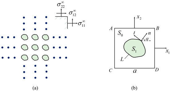
Figure 1.
(a) A nanoporous material with periodic inclusions of arbitrary shape; (b) A square RUC of the structure.
Considering the structure periodicity, every RUC should possess identical deformation mode and there should be no separation or overlap between neighboring RUCs. This indicates that the displacement increments and their gradients are uniform when across the edges of the RUC, which can be expressed as
where . Also, the equilibrium condition requires that
Since the stress components can be derived from the displacement components, Equation (3) can be used to determine the displacement increments after the remote loads are given.
At the boundary between the inclusion and matrix, a non-slippery condition is assumed which requires that the displacement be continuous when across L
The stress components, however, may experience a jump when across the interface L since the size of the inclusion may reach the nanoscale when the interface stress effect starts to play important roles. According to the well-known G-M interface stress model [12,13,14], the stress jump can be written as
where is the arc length and is the interface stress
where and are the interface Lamé constants, and is the interfacial hoop strain.
3. Solution to the Problem Using the Complex Variable Method
For plane problems, the displacements and stresses can be expressed in the coordinate system via two analytic complex functions and as [30]
where is the shear modulus, z is the complex variable , and with being the Poisson’s ratio. By using Equation (7), the displacement boundary conditions (1) and (2) that describe the structure periodicity can be expressed, respectively, as
where , , and are arbitrarily-chosen points on the edges that satisfy
At the inclusion-matrix interface, the displacement boundary condition (4) can be rewritten as
The stress boundary condition (5) can be simplified into an alternative form as
For the present plane-strain problem, the hoop strain from Equation (6) is equal to the hoop strain at the interface on either side of the bulk materials. Here we utilize the interfacial hoop strain on the matrix side which is
To deal with the arbitrary inclusion shape considered in this work, the conformal mapping function
may be introduced to map the interface boundary curve and its exterior onto the unit circle centered at the origin in an imaginary - plane and the exterior of the unit circle, respectively. In particular, points at the interface L satisfy the following mapping relation
The parameter R is related to the inclusion size and is a real number while the parameters are determined by the inclusion shape and are complex numbers. For practical calculation, the mapping (14) is usually truncated into finite series terms.
Notice that the complex potentials in the inclusion domain and can be expanded into the following series form
where a1j (j = 1…N) and b1j (j = 1…N) are unknown complex coefficients. The complex potentials in the matrix domain (which is the intersection of the exterior of the inclusion and the interior of the RUC) can be expressed as the following form according to the superposition principle
where a0j (j = 1…N), b0j (j = 1…N), c0j (j = 1…M) and d0j (j = 1…M) are unknown complex coefficients while are Faber polynomials for the square RUC that can be described as
Inserting the series forms of the complex potentials (16) and (17) into the boundary conditions (11) and (12) gives
and
where
In the above, the coefficients hij (i = 1…17) are Fourier coefficients that can be calculated as follows:
By comparing the coefficients of the two sides of (19) and (20), one set of linear equations about a1j (j = 1…N), b1j (j = 1…N), a0j (j = 1…N), b0j (j = 1…N), c0j (j = 1…M) and d0j (j = 1…M) can be obtained.
Inserting (16) and (17) into the periodic boundary conditions (8) and (9) gives
In order to address the displacement boundary conditions (23) to (26) on the RUC edges, the collocation method can be employed. This entails selecting a group of points on the RUC edges that satisfy the aforementioned boundary conditions. As long as the number of collocation points is sufficiently large, the results obtained via this method will be sufficiently accurate. It is possible to select collocation points at equal distances from each edge of the square ABCD that satisfy the following conditions:
Calculate the corresponding mapped points of the above collocation points in the - plane and insert them into the boundary conditions (23) to (26). Then another set of linear equations about a1j (j = 1…N), b1j (j = 1…N), a0j (j = 1…N), b0j (j = 1…N), c0j (j = 1…M) and d0j (j = 1…M) can be obtained. After the unknown coefficients are solved from the linear equations, the elastic field inside the RUC is then determined. Based on the solution of the elastic field, the effective stiffness of the nanocomposite can be given as follows:
To obtain the elements in the effective stiffness matrix, four different and independent loading conditions should be considered. For example, one can set , ; , ; , and , , and then utilize the symmetry of the stress tensor to obtain the corresponding displacement incremental (i = 1…4). The effective stiffness matrix directly relates the stress components and strain components. We believe this might be more convenient for engineers in practice. In fact, one can easily determine the elastic constants from the elements in the effective stiffness matrix.
4. Numerical Examples and Discussion
4.1. Verification of the Present Solution
The accuracy of the present solution shall be verified in this section from two aspects. Firstly, notice that composites usually exhibit macroscopically orthotropic behaviors and the constitutive relations for orthotropic materials under plane-strain deformation reads
Therefore, the effective stiffness matrix of the periodic nanocomposites in this work should resemble that in Equation (29). Fortunately, we have found that the stiffness elements defined in Equation (28) always satisfies and for all the numerical examples. This conclusion also indicates that we need to only consider , , and . Secondly, we compare our results for periodic nanocomposites with circular holes with the known ones by setting the parameter to be 0.001. Here, we have rewritten [31]. Since the nanocomposites with circular holes are symmetric about the and axes, we have . The comparisons of , and have been plotted in Figure 2. Good agreement guarantees the validity of the present solution.
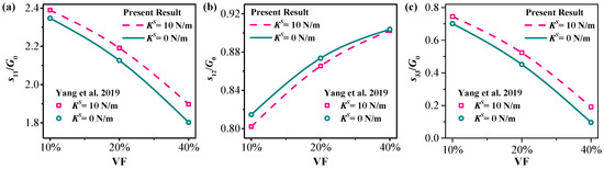
Figure 2.
Comparison of the effective stiffness matrix elements (a) , (b) and (c) of a period nanocomposite structure containing nanoscale circular holes with varying VFs and surface elasticity constants. The radius of the circular hole is 5 nm. Present results are plotted using lines (including solid and dash ones) while results by Yang et al. [32] are plotted using symbols (squares and circles).
4.2. Numerical Investigations of the Effective Stiffness of Periodic Nanocomposites
The effective stiffness of a periodic nanocomposite depends on its microstructure, including the shape, size, orientation, and volume fraction of the nanoscale inclusion, as well as the interface property and the material constant difference between the inclusion and matrix. In the following, numerical examples will be shown to investigate the influences of the above-mentioned factors. Table 1 and Table 2 list the inclusion shapes and their conformal mappings, material constants of the matrix and inclusion, and other important parameters and their values, respectively.

Table 1.
Inclusion shape and their conformal mappings.
Table 2.
Material type and material constants of the matrix and inclusion phases (on the left side) and the values of the parameters taken in the numerical examples (on the right side).
4.2.1. Investigation on the Influence of Volume Fraction (VF)
Table 3 and Table 4 present the effective stiffness elements (, , and ) with the VF of periodic nanocomposites containing elliptical and square inclusions, respectively. The constant R is set to 5 nm, the orientation angle is 0°, and the interface elasticity constant KS can assume values of 0 or 10 N/m. As evidenced in Table 3 and Table 4, an increase in VF from 0.1 to 0.3 results in a decrease in the elements for soft inclusions, indicating a compliance enhancement in the nanocomposite. Conversely, an increase in VF from 0.1 to 0.3 results in an increase in the elements for hard inclusions, implying a stiffness increase in the nanocomposite. It can thus be concluded that the impact of VF on the effective stiffness of a nanocomposite is markedly dependent upon the specific inclusion type. Furthermore, the impact of the interface stress effect is investigated by varying the interface elasticity parameter . It is observed that the elements increase when is increased from 0 to 10 N/m, indicating that the interface stress effect results in a stiffening effect. A comparison of the results presented in Table 3 and Table 4 reveals that the shape of the inclusion can also influence the effective stiffness of the nanocomposite. However, the impact of inclusion shape is considerably less pronounced compared to the effects of K S and VF, despite the fact that the stress field surrounding different shapes of nano-inclusions can exhibit notable differences [33,34]. While the influence of inclusion shape on the effective stiffness elements is relatively minor, a notable distinction emerges when comparing elliptical and square inclusions. The values of and exhibit slight differences for the elliptical inclusion but are identical for the square inclusion. This is because that the elements and roughly reflect the tension resistances of the nanocomposite in the and directions, respectively. It can be expected that the tension resistance of the nanocomposite in the direction will differ from that in the direction for elliptical inclusions, whereas it will be identical for square inclusions.
Table 3.
Variation in the effective stiffness elements with the volume fraction (VF) of periodic nanocomposites containing elliptical inclusions. The parameter R = 5 nm.
Table 4.
Variation in the effective stiffness elements with the volume fraction (VF) of periodic nanocomposites containing square inclusions. The parameter R = 5 nm.
4.2.2. Investigation on the Influence of Inclusion Size
Table 5 and Table 6 list the variation in the effective stiffness elements with inclusion size of periodic nanocomposites containing elliptical and square inclusions, respectively. The VF of inclusion is set to be 20%, the orientation angle is 0°, and the interface elasticity constant can assume values of 0 or 10 N/m. The parameter R is assumed to vary from 5 nm to 20 nm because the possible size-dependent phenomena is apparent in this range. The results show that the effective stiffness elements of the nanocomposite do not change when R increases from 5 nm to 20 nm for the case of which implies the size-independency of the effective stiffness of the nanocomposite in this case, since it means that the stress jump across the interface is zero and the problem degenerates to the traditional one. However, when the interface elasticity parameter is increased to 10 N/m, the effective stiffness elements not only become larger, but become size-dependent, increasing slightly with decreasing inclusion size, implying a stiffer composite for smaller inclusions. Moreover, the size effect gets weaker for hard inclusions when compared with soft ones.
Table 5.
Variation in the effective stiffness elements with inclusion size of periodic nanocomposites containing elliptical inclusions. The VF of inclusion is 20%.
Table 6.
Variation in the effective stiffness elements with inclusion size of periodic nanocomposites containing square inclusions. The VF of inclusion is 20%.
4.2.3. Investigation on the Influence of Orientation Angle
For orthotropic nanocomposites, it is of great importance to investigate how the orientation angle of the inclusion may affect their effective mechanical properties. Figure 3 plots the variation in the effective stiffness elements of the nanocomposite , and with the orientation angle for the square inclusion when the parameter R is set to be 5 nm and the VF to be 0.2. Notice that for the case of square inclusions, the element is always equal to due to the geometrical symmetry, which has also been demonstrated by our numerical examples (See Table 4 and Table 6). The figure shows that the elements , and hardly change with the orientation angle when . However, when is increased to 10 N/m, the variations of the elements become a little more obvious with the orientation angle. Despite that, the maximum relative change of the elements for different orientation angles is smaller than 0.2%, implying that the nanocomposite may be viewed as a transversely homogeneous material.
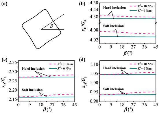
Figure 3.
The inclusion shape (a) and variation in the effective stiffness elements (b) , (c) and (d) of the nanocomposite with the orientation angle for the square inclusion.
In this study, we have assumed a non-slippery interface between the inclusion and matrix and considered the interface elasticity parameter KS to be constant during the mechanical analysis. However, molecular dynamics (MD) simulation [35] shows that for metal nanocomposites, interfacial debonding may occur due to the accumulated surface stress if the matrix is initially dislocation-free. The debonding behavior may significantly affect the interfacial displacement boundary condition between the inclusion and matrix and cause a drop in the stress–strain curve, and therefore the overall mechanical behavior of the nanocomposite. This subject is worth studying in the future.
5. Conclusions
The present investigation provides a comprehensive understanding of the effective stiffness of periodic nanocomposites with arbitrarily-shaped inclusions by examining the influence of various microstructural parameters. Our findings, derived from the complex variable method, underscore the pivotal role of the interface elasticity parameter in determining the mechanical properties of nanocomposites.
We have demonstrated that the effective stiffness of nanocomposites is markedly dependent on the interface elasticity parameter, with an increase in leading to a stiffer composite. This is attributed to the stiffening effect induced by the interface stress, which becomes increasingly significant as the inclusion size approaches the nanoscale. The size effect on the effective stiffness is also evident, with smaller inclusions resulting in a slightly stiffer composite when the interface elasticity parameter is non-zero. This size dependency is a direct consequence of the increasing ratio of surface/interfaces to the total volume of the material as it approaches the nanoscale. Furthermore, our numerical examples reveal that the shape of the inclusion, while influential, has a less pronounced impact on the effective stiffness compared to the interface stress effect and volume fraction. Notably, the orientation angle of the inclusion has a minimal effect on the effective stiffness elements, suggesting that the nanocomposite can be considered transversely homogeneous within the range of orientation angles investigated.
In summary, this study offers valuable insights into the mechanical behavior of nanocomposites and the critical factors that govern their effective stiffness. Our results emphasize the importance of considering interfacial effects and microstructural parameters in the design and optimization of nanocomposite materials for engineering applications. Future research may focus on extending this methodology to other types of nanocomposites and exploring additional factors that could influence their mechanical properties.
Author Contributions
Conceptualization, S.W., M.C. and H.Y.; Data curation, S.W.; Formal analysis, S.W.; Funding acquisition, H.Y.; Investigation, M.C. and H.L.; Methodology, H.Y.; Project administration, H.Y.; Software, S.W. and X.J.; Supervision, H.Y.; Validation, S.W. and H.L.; Visualization, X.J. and C.Y.; Writing—original draft, S.W.; Writing—review & editing, S.W., X.J., M.C., H.L., C.Y. and H.Y. All authors have read and agreed to the published version of the manuscript.
Funding
This work is supported by the National Natural Science Foundation of China (Nos. 12002004, 12202010, U2141251, 12402191); the State Key Laboratory of Mechanics and Control for Aerospace Structures (Nanjing University of Aeronautics and astronautics) (Grant No. MCAS-E-0124Y02); the Fundamental Research Funds for the Central Universities under Grant B240201115; and the Natural Science Foundation of Guangdong Province (Grant No. 2022A1515011773); the JiangXi “Double Thousand Plan” (S2021CQKJ1650); the Natural Science Foundation of Jiangsu Province (BK20210787).
Data Availability Statement
Data are contained within the article.
Conflicts of Interest
The authors declare no conflicts of interest.
References
- Wong, E.W.; Sheehan, P.E.; Lieber, C.M. Nanobeam mechanics: Elasticity, strength, and toughness of nanorods and nanotubes. Science 1997, 277, 1971–1975. [Google Scholar] [CrossRef]
- Naganuma, T.; Kagawa, Y. Effect of particle size on the optically transparent nano meter-order glass particle-dispersed epoxy matrix composites. Compos. Sci. Technol. 2002, 62, 1187–1189. [Google Scholar] [CrossRef]
- Cui, Y.; Lieber, C.M. Functional nanoscale electronic devices assembled using silicon nanowire building blocks. Science 2001, 291, 851–853. [Google Scholar] [CrossRef] [PubMed]
- Pour, G.B.; Ashourifar, H.; Aval, L.K.; Solaymani, S. CNTs-Supercapacitors: A Review of Electrode Nanocomposites Based on CNTs, Graphene, Metals, and Polymers. Symmetry 2023, 15, 1179. [Google Scholar] [CrossRef]
- Wang, Z.L.; Song, J. Piezoelectric nanogenerators based on zinc oxide nanowire arrays. Science 2006, 312, 242–246. [Google Scholar] [CrossRef]
- Almessiere, M.A.; Algarou, N.A.; Slimani, Y.; Klygach, D.S.; Baykal, A.; Korkmaz, A.D.; Zubar, T.I.; Silibin, M.V.; Vakhitov, M.G.; UI-Hamid, A.; et al. Structure, magnetic and electrodynamic properties of SrInxFe12-xO4/Ni0.5Zn0.5Fe2O4 composites at low temperature. J. Am. Ceram. Soc. 2024, 107, 4936–4948. [Google Scholar] [CrossRef]
- Matzui, L.Y.; Trukhanov, A.V.; Yakovenko, O.S.; Vovchenko, L.L.; Zagorodnii, V.V.; Oliynyk, V.V.; Borovoy, M.O.; Trukhanova, E.L.; Astapovich, K.A.; Karpinsky, D.V.; et al. Functional magnetic composites based on hexaferrites: Correlation of the composition, magnetic and high-frequency properties. Nanomaterials 2019, 9, 1720. [Google Scholar] [CrossRef] [PubMed]
- Trukhanov, S.V.; Fedotova, V.V.; Trukhanov, A.V.; Szymczak, H.; Botez, C.E. Cation ordering and magnetic properties of neodymium-barium manganites. Tech. Phys. 2008, 53, 49–54. [Google Scholar] [CrossRef]
- Trukhanov, S.V.; Trukhanov, A.V.; Kostishyn, V.G.; Panina, L.V.; Turchenko, V.A.; Kazakevich, I.S.; Trukhanov, A.V.; Trukhanova, E.L.; Natarov, V.O.; Balagurov, A.M. Thermal evolution of exchange interactions in lightly doped barium hexaferrites. J. Magn. Magn. Mater. 2017, 426, 554–562. [Google Scholar] [CrossRef]
- Trukhanov, S.V.; Trukhanov, A.V.; Kostishyn, V.G.; Zabeivorota, N.I.; Panina, L.V.; Trukhanov, A.V.; Turchenko, V.A.; Trukhanova, E.L.; Oleynik, V.V.; Yakovenko, O.S.; et al. High-frequency absorption properties of gallium weakly doped barium hexaferrites. Philos. Mag. 2019, 99, 585–605. [Google Scholar] [CrossRef]
- Poncharal, P.; Wang, Z.; Ugarte, D.; de Heer, W.A. Electrostatic deflections and electromechanical resonances of carbon nanotubes. Science 1999, 283, 1513–1516. [Google Scholar] [CrossRef] [PubMed]
- Gurtin, M.E.; Murdoch, A.I. A continuum theory of elastic material surfaces. Arch. Ration. Mech. Anal. 1975, 57, 291–323. [Google Scholar] [CrossRef]
- Gurtin, M.E.; Murdoch, A.I. Surface stress in solids. Int. J. Solids Struct. 1978, 14, 431–440. [Google Scholar] [CrossRef]
- Gurtin, M.E.; Weissmüller, J.; Larche, F. A general theory of curved deformable interfaces in solids at equilibrium. Philos. Mag. A 1998, 78, 1093–1109. [Google Scholar] [CrossRef]
- Miller, R.E.; Shenoy, V.B. Size-dependent elastic properties of nanosized structural elements. Nanotechnology 2000, 11, 139–147. [Google Scholar] [CrossRef]
- Shenoy, V.B. Size-dependent rigidities of nanosized torsional elements. Int. J. Solids Struct. 2002, 39, 4039–4052. [Google Scholar] [CrossRef]
- Sharma, P.; Ganti, S.; Bhate, N. Effect of surfaces on the size-dependent elastic state of nano-inhomogeneities. Appl. Phys. Lett. 2003, 82, 535–537. [Google Scholar] [CrossRef]
- Sharma, P.; Ganti, S. Interfacial elasticity corrections to size-dependent strain-state of embedded quantum dots. Phys. Status Solidi B Basic Solid State Phys. 2002, 234, 10–12. [Google Scholar] [CrossRef]
- Duan, H.L.; Wang, J.; Huang, Z.P.; Karihaloo, B.L. Size-dependent effective elastic constants of solids containing nano-inhomogeneities with interface stress. J. Mech. Phys. Solids 2005, 53, 1574–1596. [Google Scholar] [CrossRef]
- Chen, T.; Dvorak, G.J.; Yu, C.C. Size-dependent elastic properties of unidirectional nano-composites with interface stresses. Acta Mech. 2007, 188, 39–54. [Google Scholar] [CrossRef]
- Xiao, J.H.; Xu, Y.L.; Zhang, F.C. Evaluation of effective electroelastic properties of piezoelectric coated nano-inclusion composites with interface effect under antiplane shear. Int. J. Eng. Sci. 2013, 69, 61–68. [Google Scholar] [CrossRef]
- Wang, G.F.; Feng, X.Q.; Yu, S.W.; Nan, C.W. Interface effects on effective elastic moduli of nanocrystalline materials. Mater. Sci. Eng. A 2003, 363, 1–8. [Google Scholar] [CrossRef]
- Chen, H.; Hu, G.; Huang, Z. Effective moduli for micropolar composite with interface effect. Int. J. Solids Struct. 2007, 44, 8106–8118. [Google Scholar] [CrossRef][Green Version]
- Huang, Z.P.; Sun, L. Size-dependent effective properties of a heterogeneous material with interface energy effect: From finite deformation theory to infinitesimal strain analysis. Acta Mech. 2007, 190, 151–163. [Google Scholar] [CrossRef]
- Doan, T.; Le-Quang, H.; To, Q.-D. Effective elastic stiffness of 2D materials containing nanovoids of arbitrary shape. Int. J. Eng. Sci. 2020, 150, 103234. [Google Scholar] [CrossRef]
- Mogilevskaya, S.G.; Crouch, S.L.; Stolarski, H.K.; Benusiglio, A. Equivalent inhomogeneity method for evaluating the effective elastic properties of unidirectional mult-phase composites with surface/interface effects. Int. J. Solids Struct. 2010, 47, 407–418. [Google Scholar] [CrossRef]
- Wang, H.W.; Zhou, H.W.; Peng, R.D.; Mishnaevsky, L. Nanoreinforced polymer composites: 3D FEM modeling with effective interface concept. Compos. Sci. Technol. 2011, 71, 980–988. [Google Scholar] [CrossRef]
- Yvonnet, J.; Quang, H.L.; He, Q.C. An XFEM/level set approach to modelling surface/interface effects and to computing the size-dependent effective properties of nanocomposites. Comput. Mech. 2008, 42, 119–131. [Google Scholar] [CrossRef]
- Dai, M.; Schiavone, P.; Gao, C.F. A new method for the evaluation of the effective properties of composites containing unidirectional periodic nanofibers. Arch. Appl. Mech. 2017, 87, 647–665. [Google Scholar] [CrossRef]
- Muskhelishvili, N.I. Some Basic Problems of the Mathematical Theory of Elasticity; Noordhoff: Groningen, The Netherlands, 1953. [Google Scholar]
- Tian, L.; Rajapakse, R.K.N.D. Elastic field of an isotropic matrix with a nanoscale elliptical inhomogeneity. Int. J. Solids Struct. 2007, 44, 7988–8005. [Google Scholar] [CrossRef]
- Yang, H.B.; Wang, S.; Yu, C. Effective in-plane stiffness of unidirectional periodic nanoporous materials with surface elasticity. Z. Für Angew. Math. Phys. 2019, 70, 129. [Google Scholar] [CrossRef]
- Wang, S.; Dai, M.; Ru, C.Q.; Gao, C.F. Stress field around an arbitrarily shaped nanosized hole with surface tension. Acta Mech. 2014, 225, 3453–3462. [Google Scholar] [CrossRef]
- Dai, M.; Gao, C.F.; Ru, C.Q. Surface tension-induced stress concentration around a nanosized hole of arbitrary shape in an elastic half-plane. Meccanica 2014, 49, 2847–2859. [Google Scholar] [CrossRef]
- Cui, Y.; Chen, Z. Void initiation from interfacial debonding of spherical silicon particles inside a silicon-copper nanocomposite: A molecular dynamics study. Model. Simul. Mater. Sci. Eng. 2017, 25, 025007. [Google Scholar] [CrossRef]


Disclaimer/Publisher’s Note: The statements, opinions and data contained in all publications are solely those of the individual author(s) and contributor(s) and not of MDPI and/or the editor(s). MDPI and/or the editor(s) disclaim responsibility for any injury to people or property resulting from any ideas, methods, instructions or products referred to in the content. |
© 2024 by the authors. Licensee MDPI, Basel, Switzerland. This article is an open access article distributed under the terms and conditions of the Creative Commons Attribution (CC BY) license (https://creativecommons.org/licenses/by/4.0/).