The Effect of Fractional Order of Time Phase Delay via a Mixed Integral Equation in (2 + 1) Dimensions with an Extended Discontinuous Kernel

Abstract

It is common knowledge that studying integral equations accompanied by and related to phase delay is significant, and that significance grows when considering the problem’s time factor. Through this study, one may predict the material’s state for a short time or infer its state before beginning the investigation. In this work, a phase-lag mixed integral equation (P-MIE) with a continuous kernel in time and a singular kernel in position is studied in (2 + 1) dimensions in the space $L_2\left(\right[a,b]\times [c,d\left]\right)\times C[0,T],T<1$. The properties of fractional integrals are used to generate the mixed integral equation (MIE). Certain assumptions are considered in order to examine convergence, uniqueness of solution, and estimation error. We achieve a class of two-dimensional Fredholm integral equations (FIEs) with time-dependent coefficients after applying the separation technique. After that, we will get a linear algebraic system (LAS) in 2Ds applying the product Nystrӧm method (PNM). The convergence of the LAS’s unique solution is covered. Two applications on the MIE with a logarithmic kernel and a Carleman function are discussed to illustrate the viability and efficiency of the applied techniques. At the end, a valuable conclusion is established.

1. Introduction

With their wide range of applications in science and engineering, integral equations have piqued the curiosity of mathematicians. Recent research in the field of material phenomena has focused on a specific class of integral equations known as quadratic third-kind mixed integral equations with discontinuous kernels. Spectral relationships in this area have addressed a number of challenges, including the formulation and solution of integral equations with various kinds of singular kernels. For example, Alhazmi et al.’s work [1] examined the spectral connections and physical phenomena using a quadratic third-kind mixed integral equation with symmetric discontinuous kernels, emphasizing the complexity of these systems and their solutions. Similarly, in order to increase the knowledge and usefulness of these equations in a variety of mathematical issues, Basseem and Alalyani [2] offered solutions to nonlinear integral equations with various symmetric singular kernels. Moreover, the study of nonlinear integral equations has focused on the use of innovative numerical techniques. A block-by-block approach for nonlinear variable-order fractional of nonlinear integral equation was presented by Afiatdoust et al. [3]. An asymptotic model for mixed integral equations in location and time was presented by Jan [4], providing a solid framework for the analysis of such problems. In [5], authors applied a mathematical model of heat transport in a functionally graded thick plate in the context of Taylor’s series expansion for the dual-phase-lag heat conduction law. The author in [6] studied the time differential dual-phase-lag model of a thermoelastic material. On the other hand, many problems in mechanics, engineering, and physics can be formulated by integral equations. For example, low-frequency electromagnetic perturbation [7]. For that, many researchers pay attention to solving the integral equations with time delay problems analytically or numerically. In [8], the existence of a unique solution of Fredholm–Volterra integral equations (F-VIEs) with phase lag was discussed. Numerical solutions were considered for fractional-order linear delay differential equations via the Laplace transform technique [9]. Rostami and Maleknejad [10] used Hybrid 2-D Taylor polynomials, block pulse functions, and operational matrices of integration to discuss the solution of 2-D NV–FIPDEs with initial conditions. Nili in [11] proposed an efficient mesh-less method for MIEs with phase lag. The technique that combines quadrature rules and the Adomian method for approximating the solutions of phase lag NV-FIEs was developed in [12]. The phase-lag nonlinear integral equation was conformed to the Volterra–Hammerstein integral equation (V-HIE) of the second kind [13]. Xie [14] presented a numerical scheme to discuss the solution of fractional spatial–temporal telegraph equations with variable coefficients by applying the modified fractional Legendre wavelets. On the other hand, numerical solutions of IEs with singular kernels in one or two dimensions take their place in the research; for further details, we recommend the reader refer to references [15,16,17,18,19,20]. PNM was applied to the 2-D VIE to get a LAS in [21]. Also, the PNM was used to treat 2-D FIEs, defined on general curvilinear domains of the plane in [22].

It is known that the phase delay and the study of its behavior directly affect the prediction of how the solution behaves and the knowledge of the effect of memory on it. Also, the effect of the position kernel when it is discontinuous increases the complexity of the problem, which prompts researchers to try to find appropriate methods for these problems, which is what we are trying to address in this research paper.

Studying the treatment of P-MIE with singular kernels in the space $L_2\left(\left[a,b\right]\times \left[c,d\right]\right)\times C\left[0,T\right],\left(T<1\right)$ is the goal of the current work. First, a (2 + 1) dimensional MIE is produced by applying fractional integral characteristics and Taylor expansion on P-MIE. Numerous special types such as the logarithmic kernel, Carleman function, Cauchy kernel, and strong singular kernel, are discussed in Section 3. In Section 4, it is demonstrated that the series of solutions converges to the exact answer, proving the convergence of the MIE’s solution. The contraction theorem is used in Section 5 to show that there is a unique solution. The evidence that the convergence of the estimating error leads to the convergence of the approximation solution is covered in Section 6. Subsequently, the MIE is converted into a 2D-IEs in position with coefficients that are functions of time in Section 7 by applying separation of variables. Following the application of the convergence test, the relationship between the position kernel for the FIE in 2D and its coefficients of fractional time is found in Section 8. Section 9 uses PNM, a popular numerical technique for solving singular IEs, to construct a system of linear algebraic equations (SLAEs). Furthermore, the logarithmic kernel and the Carleman function—the two most prevalent kinds of singular kernels—are dealt with in Nyström’s technique. To show that the techniques offered are useful and efficient in solving P-MIE, numerical applications are solved in Section 10. The Maple 18 software is used to get all the results. The results are also discussed, analyzed and debated. Lastly, the end of this work mentions several significant issues pertaining to this study.

2. Formulation of the Problem

In this section, the authors impose an integral problem in space (2 + 1) with a singular position’s kernel. The integral equation’s time exhibits phase delay is applied on time to obtain a fractional differential equation. Using the characteristics of fractional integrals, the researchers were able to obtain a MIE. Here we get at an important rule: integral equations with phase delay transform into mixed integral equations of Volterra-type appointed to time and Fredholm-type specific to position.

Consider the P-MIE, in the space $L_2\left(\left[a,b\right]\times \left[c,d\right]\right)\times C\left[0,T\right],\left(T<1\right),$

$$\mathsf{\Phi }\left(u,v;t-q\right)=f\left(u,v;t\right)+\lambda {\int }_0^t{\int }_c^d{\int }_a^{b}g\left(t,\tau \right)S\left(\left|u-\delta \right|,\left|v-\gamma \right|\right)\mathsf{\Phi }\left(\delta ,\gamma ;\tau \right)d\delta d\gamma d\tau , q\ll 1,$$

(1)

with initial conditions

$$\mathsf{\Phi }\left(u,v;0\right)=V_1\left(u,v\right), {\left.{\displaystyle \frac{\partial \mathsf{\Phi }\left(u,v;t\right)}{\partial t}}\right]}_{t=0}=V_2(u,v).$$

(2)

where $f(u,v;t)$ is a free term, $\lambda$ is a parameter, $g(t,\tau )$ is a continuous function of time and represents the kernel of Volterra integral term, while $S(\left|u-\delta \right|,\left|v-\gamma \right|)$ is the position kernel that have two singularities and $\mathsf{\Phi }(u,v;t)$ is the unknown function.

We use Taylor’s expansion, in the fractional science, to obtain

$$\begin{gathered} \mathsf{\Phi }\left(u,v;t-q\right)\cong \mathsf{\Phi }\left(u,v;t\right)-{\displaystyle \frac{q^{\alpha }}{\mathsf{\Gamma }\left(\alpha +1\right)}}{\displaystyle \frac{{\partial }^{\alpha }}{\partial t^{\alpha }}}\mathsf{\Phi }\left(u,v;t\right)+{\displaystyle \frac{q^{\alpha +1}}{\mathsf{\Gamma }\left(\alpha +2\right)}}{\displaystyle \frac{{\partial }^{\alpha +1}}{\partial t^{\alpha +1}}}\mathsf{\Phi }\left(u,v;t\right) \\ -{\displaystyle \frac{q^{\alpha +2}}{\mathsf{\Gamma }\left(\alpha +3\right)}}{\displaystyle \frac{{\partial }^{\alpha +2}}{\partial t^{\alpha +2}}}\mathsf{\Phi }\left(u,v;t\right)+\dots +{\left(-1\right)}^n{\displaystyle \frac{q^{\alpha +\left(n-1\right)}}{\mathsf{\Gamma }\left(\alpha +n\right)}}{\displaystyle \frac{{\partial }^{\alpha +n-1}}{\partial t^{\alpha +n-1}}}\mathsf{\Phi }\left(u,v;t\right), \left(n-1\right)<\alpha <n, \end{gathered}$$

(3)

for simplicity, we focus the expansion to the following approximation

$$\mathsf{\Phi }\left(u,v;t-q\right)\cong \mathsf{\Phi }\left(u,v;t\right)-{\displaystyle \frac{q^{\alpha }}{\mathsf{\Gamma }\left(\alpha +1\right)}}{\displaystyle \frac{{\partial }^{\alpha }\mathsf{\Phi }\left(u,v;t\right)}{\partial t^{\alpha }}}+{\displaystyle \frac{q^{\alpha +1}}{\mathsf{\Gamma }\left(\alpha +2\right)}}{\displaystyle \frac{{\partial }^{\alpha +1}\mathsf{\Phi }\left(u,v;t\right)}{\partial t^{\alpha +1}}}.$$

(4)

In Equation (4), we consider the phase-lag of O($q^{\alpha +2})\to 0.$

Using Riemann–Liouville fractional integral properties

$${}_{a}I_t^{\alpha }u\left(x\right)={\displaystyle \frac{1}{\mathsf{\Gamma }\left(\alpha \right)}}{\int }_a^x{\left(x-t\right)}^{\alpha -1}u\left(t\right)dt,$$

(5)

$$\left(\left({}_{a}I_t^{\alpha }{}_{a}I_t^{\beta }\right)u\right)\left(x\right)=\left({}_{a}I_t^{\alpha +\beta }u\right)\left(x\right)={\displaystyle \frac{1}{\mathsf{\Gamma }\left(\alpha +\beta \right)}}{\int }_a^x{\left(x-t\right)}^{\alpha +\beta -1}u\left(t\right)dt,$$

(6)

and Cauchy’s formula for repeated integration

$${\int }_0^t{\int }_0^{{\tau }_n}\dots {\int }_0^{{\tau }_3}{\int }_0^{{\tau }_2}u\left({\tau }_1\right)d{\tau }_{1}d{\tau }_2\dots d{\tau }_{n-1}d{\tau }_n={\displaystyle \frac{1}{\left(n-1\right)!}}{\int }_0^t{\left(t-\tau \right)}^{n-1}u\left(\tau \right)d\tau ,n\in \mathbb{N}.$$

(7)

In the view of Equations (4–7) and Equation (1), we have

$$\begin{gathered} {\mu }_1\mathsf{\Phi }\left(u,v;t\right)-{\mu }_2{\int }_0^t\left(1-{\displaystyle \frac{\alpha {\left(t-\tau \right)}^{\alpha }}{q^{\alpha }}}\right)\mathsf{\Phi }\left(u,v;\tau \right)d\tau \\ -{\mu }_3{\int }_0^t{\left(t-\tau \right)}^{\alpha +1}g\left(t,\tau \right){\int }_c^d{\int }_a^{b}S\left(\left|u-\delta ,v-\gamma \right|\right)\mathsf{\Phi }\left(\delta ,\gamma ;\tau \right)d\delta d\gamma d\tau =F\left(u,v;t\right), \end{gathered}$$

(8)

where,

$$F\left(u,v;t\right)={\displaystyle \frac{1}{\mathsf{\Gamma }\left(\alpha +1\right) }}{\int }_0^t{\left(t-\tau \right)}^{\alpha }f\left(u,v;\tau \right)d\tau +{\displaystyle \frac{q^{\alpha +1}}{\mathsf{\Gamma }\left(\alpha +2\right)}}\left({\displaystyle \frac{{V_2\left(u,v\right)T}^{\alpha }}{\mathsf{\Gamma }\left(\alpha +1\right)}}+V_1\left(u,v\right)\right),$$

and

$${\mu }_1={\displaystyle \frac{q^{\alpha +1}}{\mathsf{\Gamma }\left(\alpha +2\right)}}, {\mu }_2={\displaystyle \frac{q^{\alpha }}{\mathsf{\Gamma }\left(\alpha +1\right)}}, {\mu }_3= {\displaystyle \frac{\lambda }{ \Gamma \left(\alpha \right)}} .$$

(9)

The Formula (8) represents a MIE in (2 + 1) dimensions. This equation is equivalent to the P-MIE (1).

We need to demonstrate that there is a good solution to this equation before we are allowed to begin picking on methods to solve it. For this, we assume the following assumptions:

(i)

In $L_2\left(\right[a,b]\times [c,d\left]\right),$ the kernel of position satisfies

$${\left\{{\int }_c^d{\int }_c^d\left\{{\int }_a^b{\int }_a^b{S}^2(\left|u-\delta \right|,\left|v-\gamma \right|)dud\delta \right\}dvd\gamma \right\}}^{{\displaystyle \frac{1}{2}}}\le C, \left(C \mathrm{i}\mathrm{s} \mathrm{c}\mathrm{o}\mathrm{n}\mathrm{s}\mathrm{t}\mathrm{a}\mathrm{n}\mathrm{t}\right).$$

(ii)

The two functions $V_i\left(x,y\right),$ for the two constants $B_i, i=\left\{1, 2\right\}$ satisfy the following:

$$\left|V_1\left(u,v\right)\right|\le B_1, \mathrm{and} \left|V_2\left(u,v\right)\right|\le B_2 .$$

(iii)

The continuous function $g(t,\tau )$ in time satisfies for a constant $G,$

$$\underset{0\le t\le T}{\mathrm{m}\mathrm{a}\mathrm{x}}\left|{\int }_0^t{\left(t-\tau \right)}^{\alpha +1}g\left(t,\tau \right)d\tau \right|\le {\displaystyle \frac{T^{\alpha +2}}{\alpha +2}} G.$$

(iv)

The normality of the given function $f\left(u,v,t\right)$ in the space $L_2\left(\left[a,b\right]\times \left[c,d\right]\right)\times C\left[0,T\right]$ satisfies

$$‖f\left(u,v,t\right)‖=\underset{0\le t\le T}{\max }\left\{{\int }_0^t{\left\{{\int }_c^d{\int }_a^b{f}^2\left(u,v;\tau \right)dudv\right\}}^{1/2}d\tau \right\}\le L, L \mathrm{i}\mathrm{s} \mathrm{a} \mathrm{c}\mathrm{o}\mathrm{n}\mathrm{s}\mathrm{t}\mathrm{a}\mathrm{n}\mathrm{t}.$$

3. Special Cases from the General Singular Kernel

Many special cases can be derived from the general kernel $S\left(\left|u-\delta \right|,\left|v-\gamma \right|\right).$

• Case 1. Weak singular kernels

(i)

The Logarithmic kernels forms $S\left(\left|u-\delta \right|,\left|v-\gamma \right|\right)$ can take one of the following forms

(i-1)

$S\left(\left|u-\delta \right|,\left|v-\gamma \right|\right)=\mathrm{l}\mathrm{n}\left(\left|u-\delta \right|\right)\times \mathrm{l}\mathrm{n}\left(\left|v-\gamma \right|\right),$

(i-2)

$S\left(\left|u-\delta \right|,\left|v-\gamma \right|\right)=\mathrm{l}\mathrm{n}\left(\left|u-\delta \right|\right)\pm \mathrm{l}\mathrm{n}\left(\left|v-\gamma \right|\right).$

(ii)

Carleman functions forms

(ii-1)

$S\left(\left|u-\delta \right|,\left|v-\gamma \right|\right)={\left|u-\delta \right|}^{-{\beta }_1}.{\left|v-\gamma \right|}^{-{\beta }_2}, \left(0<{\beta }_1,{\beta }_2<1\right),$

(ii-2)

$S\left(\left|u-\delta \right|,\left|v-\gamma \right|\right)={\left|u-\delta \right|}^{-{\beta }_1}\pm {\left|v-\gamma \right|}^{-{\beta }_2}. \left(0<{\beta }_1,{\beta }_2<1\right)$

(iii)

Logarithmic-Carleman kernels forms

(iii-1)

$S\left(\left|u-\delta \right|,\left|v-\gamma \right|\right)=\mathrm{l}\mathrm{n}\left(\left|u-\delta \right|\right)\times {\left|v-\gamma \right|}^{-{\beta }_2},$

(iii-2)

$S\left(\left|u-\delta \right|,\left|v-\gamma \right|\right)={\left|u-\delta \right|}^{-{\beta }_1}.\mathrm{l}\mathrm{n}\left(\left|v-\gamma \right|\right).$

• Case 2. Cauchy singular kernel

$$S\left(\left|u-\delta \right|,\left|v-\gamma \right|\right)={\displaystyle \frac{1}{\left|u-\delta \right|\left|v-\gamma \right|}},$$

• Case 3. Strong singular kernel

$$S\left(\left|u-\delta \right|,\left|v-\gamma \right|\right)={\displaystyle \frac{1}{(u-{\delta )}^2{(v-\gamma )}^2}}.$$

The researcher can find many other mixed and singular cases between the three types.

4. The Convergence Procedure

To discuss the convergence of Equation (8), we construct a sequence of solutions $\{{\mathsf{\Phi }}_i\left(u,v; \mathrm{t}\right){\}}_{i=0}^{\mathrm{\infty }}.$ Then, we pick up two solutions {${\mathsf{\Phi }}_n\left(u,v,t\right),{\mathsf{\Phi }}_{n-1}\left(u,v,t\right)\}$ such that

$$\begin{gathered} {\mu }_1{\mathsf{\Phi }}_n\left(u,v,t\right)-{\mu }_2{\int }_0^t\left(1-{\displaystyle \frac{\alpha }{q^{\alpha }}}{\left(t-\tau \right)}^{\alpha }\right){\mathsf{\Phi }}_{n-1}\left(u,v,\tau \right)d\tau -{\mu }_3 \\ \times {\int }_0^t{\int }_c^d{\int }_a^b{\left(t-\tau \right)}^{\alpha +1}g\left(t,\tau \right)S\left(\left|\left.u-\zeta \right|,\left|v-\eta \right.\right|\right){\mathsf{\Phi }}_{n-1}\left(\zeta ,\eta ;\tau \right)d\zeta d\eta d\tau =F\left(u,v;t\right), \\ {\mu }_1{\mathsf{\Phi }}_{n-1}\left(u,v,t\right)-{\mu }_2{\int }_0^t\left(1-{\displaystyle \frac{\alpha }{q^{\alpha }}}{\left(t-\tau \right)}^{\alpha }\right){\mathsf{\Phi }}_{n-2}\left(u,v,\tau \right)d\tau -{\mu }_3 \\ \times {\int }_0^t{\int }_c^d{\int }_a^b{\left(t-\tau \right)}^{\alpha +1}g\left(t,\tau \right)S\left(\left|\left.u-\zeta \right|,\left|v-\eta \right.\right|\right){\mathsf{\Phi }}_{n-2}\left(\zeta ,\eta ;\tau \right)d\zeta d\eta d\tau =F\left(u,v;t\right). \end{gathered}$$

(10)

Then, assume

$${\mathrm{H}}_n\left(u,v,t\right)={\mathsf{\Phi }}_n\left(u,v,t\right)-{\mathsf{\Phi }}_{n-1}\left(u,v,t\right),{\mathrm{H}}_0\left(u,v,t\right)=F\left(u,v,t\right),$$

which yields

$${\mathsf{\Phi }}_n\left(u,v;t\right)=\sum _{j=0}^n{\mathrm{H}}_j\left(u,v;t\right).$$

(11)

In what follows, we shall demonstrate that this sequence of solutions converges to the exact solution.

Lemma 1.

Under the assumptions (i)–(iv), the infinite series ${\sum }_{i=0}^{\infty }{H}_i(u,v; t)$ is uniformly convergent to a continuous solution function  $\Phi \left(u,v; t\right).$

Proof. 

From Equation $\left(10\right),$ after using Equation (11), we write

$$\begin{gathered} {\mu }_1{\mathrm{H}}_n\left(u,v,t\right)={\mu }_2{\int }_0^t\left(1-{\displaystyle \frac{\alpha }{q^{\alpha }}}{\left(t-\tau \right)}^{\alpha }\right){\mathrm{H}}_{n-1}\left(u,v;\tau \right)d\tau \\ +{\mu }_3{\int }_0^t{\int }_c^d{\int }_a^b{\left(t-\tau \right)}^{\alpha +1}g\left(t,\tau \right)S\left(\left|\left.u-\zeta \right|,\left|v-\eta \right.\right|\right)H_{n-1}\left(\delta ,\gamma ;\tau \right)d\delta d\gamma d\tau . \end{gathered}$$

(12)

Formula (12), after using the Picard method under the assumptions (i–iv), transforms into

$$‖{\mathrm{H}}_n\left(u,v,t\right)‖\le \rho ‖{\mathrm{H}}_{n-1}\left(u,v,t\right)‖,\hspace{1em}\rho ={\displaystyle \frac{\left(\left|{\mu }_2\left(T-\frac{\alpha T^{\alpha +1}}{\left(\alpha +1\right)q^{\alpha }}\right)\right|+\left|{\mu }_{3}C\frac{T^{\alpha +2}}{\alpha +2}G\right|\right)}{\left|{\mu }_1\right|}}.$$

By induction, we have

$$‖{\mathrm{H}}_n\left(u,v,t\right)‖\le {\rho }^n\mathrm{\wp },$$

The inequality, after taking the limit of both sides and using Equation (11), gives

$$\mathsf{\Phi }\left(u,v;t\right)=\underset{n\to \mathrm{\infty }}{\lim }{\mathsf{\Phi }}_n\left(u,v;t\right)=\sum _{n=0}^{\mathrm{\infty }}‖{\mathrm{H}}_n\left(u,v,t\right)‖\le \sum _{n=0}^{\mathrm{\infty }}{\rho }^n\mathrm{\wp },$$

(13)

where

$$‖F\left(u,v,t\right)‖\le \mathrm{\wp }, \mathrm{\wp }={\displaystyle \frac{1}{\mathsf{\Gamma }\left(2+\alpha \right)}}\left\{\alpha L{T}^{\alpha +1}+{\displaystyle \frac{T^{\alpha }{q}^{1+\alpha }}{\mathsf{\Gamma }\left(1+\alpha \right)}}{B}_2+q^{1+\alpha }{B}_1\right\}.$$

(14)

The sequence $\left\{{\mathrm{H}}_n\left(u,v;t\right)\right\}$ converges under this constraint when condition (13) is met, thus we write

$${‖\mathsf{\Phi }\left(u,v;t\right)‖}_H={\sum }_{n=0}^{\mathrm{\infty }}‖{\mathrm{H}}_n\left(u,v;t\right)‖\le \mathrm{\wp }{\left[1-\rho \right]}^{-1}.$$

(15)

Hence, the solution’s convergence is proved.

The inequality (15) leads us to decide that $\rho <1,$ i.e.,

$$\rho ={\displaystyle \frac{T}{q^{\alpha +1}}}\left[\left(1+\alpha \right)q^{\alpha }-\alpha T^{\alpha }+\lambda CG{T}^{\alpha +1}{\displaystyle \frac{\alpha \left(1+\alpha \right)}{\left(2+\alpha \right)}}\right]<1.$$

(16)

The previous inequality (15) leads to the condition

$$T\left[\left(1+\alpha \right)q^{\alpha }+{\displaystyle \frac{\alpha \left(1+\alpha \right)}{\left(2+\alpha \right)}}\lambda C G T^{\alpha +1}\right]<q^{\alpha +1}+\alpha T^{\alpha +1}.$$

(17)

The MIE with a backward time delay may be solved by using relation (17) as the convergence condition. The negative delay equation is only valid on extremely tiny periods until the condition is satisfied, as it is evident from (16) that the greatest time T must be small. In other words, the time delay is only a certain amount that occurs throughout $[t-q,t]$. □

5. Existence and Uniqueness Solution of a Phase-Lag Mixed Integral Equation

To discuss the existence of a unique solution of Equation (1), write (8) in the integral operator form

$$\mathrm{K}\mathsf{\Phi }\left(u,v;t\right)=Q\mathsf{\Phi }\left(u,v;t\right)+{{\displaystyle \frac{1}{\mu }}}_{1}F\left(u,v;t\right) ,$$

(18)

where, we assume

$$Q\mathsf{\Phi }\left(u,v;t\right)=N\mathsf{\Phi }\left(u,v;t\right)+M\mathsf{\Phi }\left(u,v;t\right)$$

(19)

$$N\mathsf{\Phi }\left(u,v;t\right)={\displaystyle \frac{{\mu }_2}{{\mu }_1}}{\int }_0^t\left(1+{\displaystyle \frac{\alpha }{q^{\alpha }}}{\left(t-\tau \right)}^{\alpha }\right)\mathsf{\Phi }\left(u,v;\tau \right)d\tau ,$$

$$M\mathsf{\Phi }\left(u,v;t\right)={\displaystyle \frac{{\mu }_3}{{\mu }_1}}{\int }_0^t{\left(t-\tau \right)}^{\alpha +1}g\left(t,\tau \right){\int }_c^d{\int }_a^{b}S\left(\left|\left.u-\delta \right|,\left|v-\gamma \right.\right|\right)\mathsf{\Phi }\left(\delta ,\gamma ;\tau \right)d\delta d\gamma d\tau .$$

(20)

Here, in Equations (18)–(20) $\mathrm{K}\mathsf{\Phi }\left(u,v;t\right),Q\mathsf{\Phi }\left(u,v;t\right),N\mathsf{\Phi }\left(u,v;t\right),$ and $M\mathsf{\Phi }\left(u,v;t\right)$ are linear operators.

In view of the Banach fixed point theorem, we prove the following theorem.

Theorem 1.

The P-MIE (1) has an existence and unique solution, under the convergence condition (16).

Proof. 

The following lemmas must be proven in order to prove the theorem: □

Lemma 2.

Under (i)–(iv), the space $L_2\left(\left[a,b\right]\times \left[c,d\right]\right)\times C\left[0,T\right],T<1$ is mapped into itself by the integral operator (18).

Proof. 

For this, write

$$‖\mathrm{K}\mathsf{\Phi }\left(u,v;t\right)‖\le ‖Q\mathsf{\Phi }\left(u,v;t\right)‖+{{\displaystyle \frac{1}{\mu }}}_1‖F\left(u,v;t\right)‖,$$

(21)

where

$$‖Q\mathsf{\Phi }\left(u,v;t\right)‖\le ‖N\mathsf{\Phi }\left(u,v;t\right)‖+‖M\mathsf{\Phi }\left(u,v;t\right)‖$$

$$\begin{array}{c}\le ‖{\displaystyle \frac{{\mu }_2}{{\mu }_1}}{\int }_0^t\left(1+{\displaystyle \frac{\alpha }{q^{\alpha }}}{\left(t-\tau \right)}^{\alpha }\right)\mathsf{\Phi }\left(u,v;\tau \right)d\tau ‖\hfill \\ +‖{\displaystyle \frac{{\mu }_3}{{\mu }_1}}{\int }_0^t{\left(t-\tau \right)}^{\alpha +1}g\left(t,\tau \right){\int }_c^d{\int }_a^{b}S\left(\left|\left.u-\delta \right|,\left|v-\gamma \right.\right|\right)\mathsf{\Phi }\left(\delta ,\gamma ;\tau \right)d\delta d\gamma d\tau ‖.\hfill \end{array}$$

Applying conditions (i)–(iii), we have

$$‖Q\mathsf{\Phi }\left(u,v;t\right)‖\le \left|{\displaystyle \frac{{\mu }_2}{{\mu }_1}}\left(T-{\displaystyle \frac{\alpha T^{\alpha +1}}{\left(\alpha +1\right)q^{\alpha }}}\right)\right|‖\mathsf{\Phi }\left(u,v;t\right)‖+\left|{\displaystyle \frac{{\mu }_3}{{\mu }_1}} C{\displaystyle \frac{T^{\alpha +2}}{\left(\alpha +2\right)}}G\right|‖\mathsf{\Phi }\left(u,v;t\right)‖,$$

after using the values of ${\mu }_1,{\mu }_2,{\mu }_{3, }$ we have

$$‖Q\mathsf{\Phi }\left(u,v,t\right)‖\le {\displaystyle \frac{T}{q^{\alpha +1}}}\left[\left(1+\alpha \right)q^{\alpha }-\alpha T^{\alpha }+{\displaystyle \frac{\alpha \left(1+\alpha \right)}{\left(2+\alpha \right)}}\lambda CG{T}^{\alpha +1}\right]‖\mathsf{\Phi }\left(u,v;t\right)‖.$$

(22)

Hence, the operator $Q$ is bounded. Moreover, after using (22) in inequality (21), we get

$$\begin{gathered} ‖\mathrm{K}\mathsf{\Phi }\left(u,v,t\right)‖\le {\displaystyle \frac{T}{q^{1+\alpha }}}\left[\left(1+\alpha \right)q^{\alpha }-\alpha T^{\alpha }+{\displaystyle \frac{\alpha \left(1+\alpha \right)}{\left(2+\alpha \right)}}\lambda CG{T}^{\alpha +1}\right]‖\mathsf{\Phi }\left(u,v;t\right)‖ \\ +{\displaystyle \frac{1}{q^{1+\alpha }}}\left\{\alpha L{T}^{\alpha +1}+q^{1+\alpha }\left({\displaystyle \frac{T^{\alpha }}{\mathsf{\Gamma }\left(1+\alpha \right)}}{B}_2+B_1\right)\right\}. \end{gathered}$$

(23)

From (23) we can deduce the relation

$$\mathcal{o}={\displaystyle \frac{[\alpha L{T}^{\alpha +1}+T^{\alpha }{q}^{1+\alpha }\{{\mathsf{\Gamma }\left(1+\mathsf{\alpha }\right)\}}^{-1}{B}_2+q^{1+\alpha }{B}_1]}{\left[q^{\alpha +1}-T\left\{\left(1+\alpha \right)q^{\alpha }-\alpha T^{\alpha }+\alpha \left(1+\alpha \right) {\left(\left(2+\alpha \right)\right)}^{-1}\lambda CG{T}^{\alpha +1}\right\}\right]}} ,$$

which simplifies as

$$\mathcal{o}={\displaystyle \frac{\wp }{{\mu }_1(1-\rho )}} .$$

(24)

We conclude from (24) that the operator $\mathrm{K}$ maps the ball $B_{\mathcal{o}}$ of radius $\mathcal{o}$ in the space $L_2\left(\right[a,b]\times [c,d\left]\right)\times C[0,T]$ into itself. Moreover, under the condition $\rho <1,$ the inequality (23) shows that the operator $\mathrm{K}$ is bounded. □

Lemma 3.

Under (i)–(iv) the integral operator (19) is continuous and is a conteraction mapping

Proof. 

Assume two different solution ${\mathsf{\Phi }}_1\left(u,v;t\right),{\mathsf{\Phi }}_2\left(u,v;t\right),$ hence we have

$$‖Q{\mathsf{\Phi }}_1\left(u,v,t\right)-Q{\mathsf{\Phi }}_2\left(u,v,t\right)‖$$

$$\le {\displaystyle \frac{T}{q^{\alpha +1}}} \left[\left(1+\alpha \right)q^{\alpha }-\alpha T^{\alpha }+{\displaystyle \frac{\alpha \left(1+\alpha \right)}{\left(2+\alpha \right)}}\lambda CG{T}^{\alpha +1}\right]‖{\mathsf{\Phi }}_1\left(u,v:t\right)-{\mathsf{\Phi }}_2\left(u,v:t\right)‖,$$

And it might alternatively be written as

$$‖Q{\mathsf{\Phi }}_1\left(u,v;t\right)-Q{\mathsf{\Phi }}_2\left(u,v;t\right)‖\le \rho ‖{\mathsf{\Phi }}_1\left(u,v:t\right)-{\mathsf{\Phi }}_2\left(u,v:t\right)‖.$$

The above inequality leads to the continuity of the integral operator, then under the condition of convergence (16), ($\rho <1),$ we have a contraction mapping that leading to a unique solution. Hence, Theorem 1 is proven. □

6. Error Analysis and Stability

Three fundamental concepts are necessary to understand while examining approximate solutions in general and applying computer programs to find the results. These fundamentals include the degree of approximation, the approximate solution’s methodology, and, lastly, the computation program’s mistake. Additionally, we need to be mindful of the behavioral synchronization that exists between the error function and the unknown function, which is the effort function that has to be estimated. Both the unique solution and the two functions show the same behavior in terms of convergence.

In order to demonstrate the convergence of the error, we suppose that there exists a function ${\mathrm{F}}_n\left(x,y;t\right)$ for ${\mathsf{\Phi }}_n\left(x,y;t\right)$, which is an approximate solution of Equation (8). As a result, we have

$$\begin{gathered} {\mu }_1{\mathsf{\Phi }}_n\left(u,v;t\right)-{\mu }_2{\int }_0^t\left(1-{\displaystyle \frac{\alpha }{q^{\alpha }}}{\left(t-\tau \right)}^{\alpha }\right){\mathsf{\Phi }}_n\left(u,v;\tau \right)d\tau \\ -{\mu }_3{\int }_0^t{\int }_c^d{\int }_a^b{\left(t-\tau \right)}^{\alpha +1}g\left(t,\tau \right)S\left(\left|\left.u-\delta \right|,\left|v-\gamma \right.\right|\right){\mathsf{\Phi }}_n\left(\delta ,\gamma ;\tau \right)d\delta d\gamma d\tau =F_n\left(u,v;t\right). \end{gathered}$$

(25)

Hence, from (8) and (25) we have

$$\begin{gathered} {\mathrm{R}}_n\left(u,v;t\right)={\displaystyle \frac{{\mu }_2}{{\mu }_1}}{\int }_0^t\left(1-{\displaystyle \frac{\alpha }{q^{\alpha }}}{\left(t-\tau \right)}^{\alpha }\right){\mathrm{R}}_n\left(u,v;\tau \right)d\tau + \\ {\displaystyle \frac{{\mu }_3}{{\mu }_1}}{\int }_0^t{\int }_c^d{\int }_a^b{\left(t-\tau \right)}^{\alpha +1}g\left(t,\tau \right)S\left(\left|\left.u-\delta \right|,\left|v-\gamma \right.\right|\right){\mathrm{R}}_n\left(\delta ,\gamma ;\tau \right)d\delta d\gamma d\tau +{\displaystyle \frac{1}{{\mu }_1}}{Z}_n\left(u,v;t\right), \end{gathered}$$

(26)

where

$${\mathrm{R}}_n\left(u,v;t\right)=\mathsf{\Phi }\left(u,v;t\right)-{\mathsf{\Phi }}_n\left(u,v;t\right), {\mathrm{Z}}_n\left(u,v;t\right) =F\left(u,v;t\right)-{\mathrm{F}}_n\left(u,v;t\right).$$

(27)

Construct a sequence of error equations $\{{\left(R_n\right)}_i\left(u,v; \mathrm{t}\right){\}}_{i=0}^{\infty }.$ Then, we pick up to error functions {$({\mathrm{R}}_n{)}_m\left(u,v,t\right),({\mathrm{R}}_n{)}_{m-1}\left(u,v,t\right)\}$ such that they satisfy Equation (26). Hence, we have

$$\begin{gathered} {({\mathrm{E}}_n)}_m\left(u,v;t\right)={\displaystyle \frac{{\mu }_2}{{\mu }_1}}{\int }_0^t\left(1-{\displaystyle \frac{\alpha }{q^{\alpha }}}{\left(t-\tau \right)}^{\alpha }\right){({\mathrm{E}}_n)}_{m-1}\left(u,v;\tau \right)d\tau + \\ {\displaystyle \frac{{\mu }_3}{{\mu }_1}}{\int }_0^t{\int }_c^d{\int }_a^b{\left(t-\tau \right)}^{\alpha +1}g\left(t,\tau \right)S\left(\left|\left.u-\delta \right|,\left|v-\gamma \right.\right|\right)({\mathrm{E}}_n{)}_{m-1}\left(\delta ,\gamma ;\tau \right)d\delta d\gamma d\tau , \end{gathered}$$

(28)

where

$$({\mathrm{E}}_n{)}_m\left(u,v,t\right)=({\mathrm{R}}_n{)}_m\left(u,v,t\right)-({\mathrm{R}}_n{)}_m\left(u,v,t\right), ({\mathrm{E}}_n{)}_0\left(u,v,t\right)={\displaystyle \frac{1}{{\mu }_1}}{Z}_n\left(u,v;t\right) ,$$

and

$$({\mathrm{R}}_n{)}_m\left(u,v;t\right)=\sum _{i=0}^m({\mathrm{E}}_n{)}_i\left(u,v;t\right).$$

(29)

It is obvious that the error corresponds to the same integral equation principle with the same time and position kernels. We may talk about the convergence and uniqueness of the error under the same theorem assumptions.

Lemma 4.

The infinite series $\sum _{i=0}^{\infty }(E_n{)}_i\left(u,v;t\right),$ under the assumptions (i)–(v), converges uniformly to $R_n.$

Proof. 

Taking the norm of both sides of Equation (28), to have

$$\begin{gathered} ‖({\mathrm{E}}_n{)}_m\left(u,v,t\right)‖\le \rho ‖({\mathrm{E}}_n{)}_{m-1}\left(u,v,t\right)‖, \\ \rho ={\displaystyle \frac{\left(\left|\left(\alpha +2\right)q^{\alpha }\left(\left(\alpha +1\right)q^{\alpha }T-\alpha T^{\alpha +1}\right)\right|+\left|\lambda \alpha (\alpha +1)C\frac{T^{\alpha +2}}{\alpha +2}G\right|\right)}{\left(\alpha +2\right)q^{\alpha +1}}}. \end{gathered}$$

By induction, we have

$$‖({\mathrm{E}}_n{)}_m\left(u,v,t\right)‖\le {\rho }^m{\displaystyle \frac{\left(\mathsf{\alpha }+2\right) T^{\alpha +1}‖f\left(u,v;t\right)-f_m\left(u,v;t\right)‖}{q^{\alpha +1}}},$$

(30)

taking the sum as $m=0$ to $m\to \infty ,$ we have

$$\sum _{m=0}^{\infty }‖({\mathrm{E}}_n{)}_m\left(u,v,t\right)‖\le {\displaystyle \frac{\left(\mathsf{\alpha }+2\right) T^{\alpha +1}‖f\left(u,v;t\right)-f_m\left(u,v;t\right)‖}{q^{\alpha +1}}}\sum _{m=0}^{\infty }{\rho }^m.$$

Finally, we have

$$‖{\mathrm{R}}_n\left(u,v,t\right)‖\le {\left(1-\rho \right)}^{-1}{\displaystyle \frac{\left(\mathsf{\alpha }+2\right) T^{\alpha +1}‖f\left(u,v;t\right)-f_n\left(u,v;t\right)‖}{q^{\alpha +1}}},$$

(31)

which prove the convergence of the error under the condition $0<\rho <1$. □

Lemma 5.

The error is vanishing as  $n\to \infty$.

Proof. 

This lemma can be proved directly from Equation (31), where at $\mathrm{n}\to \mathrm{\infty }$, we have $f\left(u,v;t\right)=f_n\left(u,v;t\right)$, hence ${‖{\mathrm{R}}_n\left(u,v,t\right)‖}_{\mathrm{n}\to \mathrm{\infty }}\to 0.$ □

Theorem 2.

(without proof)

The error equation ${\mathrm{R}}_n\left(u,v,t\right)$ of Equation (26) has a unique representation.

The proof can be easily obtained after writing Equation (26) in the integral operator form

$${\tilde{\mathrm{K}}\mathrm{R}}_n\left(u,v;t\right)={\displaystyle \frac{1}{{\mu }_1}}{Z}_n\left(u,v;t\right)+\overline{Q}{\mathrm{R}}_n\left(u,v;t\right),$$

$$\overline{Q}{\mathrm{R}}_n\left(u,v;t\right)=\overline{N}{\mathrm{R}}_n\left(u,v;t\right)+\overline{M}{\mathrm{R}}_n\left(u,v;t\right),$$

where

$$\overline{N}{\mathrm{R}}_n\left(u,v;t\right)={\displaystyle \frac{{\mu }_2}{{\mu }_1}}{\int }_0^t\left(1-{\displaystyle \frac{\alpha }{q^{\alpha }}}{\left(t-\tau \right)}^{\alpha }\right){\mathrm{R}}_n\left(u,v;\tau \right)d\tau ,$$

$$\overline{M}{\mathrm{R}}_n\left(u,v;t\right)={\displaystyle \frac{{\mu }_3}{{\mu }_1}}{\int }_0^t{\int }_c^d{\int }_a^b{\left(t-\tau \right)}^{\alpha +1}g\left(t,\tau \right)S\left(\left|\left.u-\delta \right|,\left|v-\gamma \right.\right|\right){\mathrm{R}}_n\left(\delta ,\gamma ;\tau \right)d\delta d\gamma d\tau ,$$

Then, following the same way of Theorem 1, the proof is obtained.

One way is to divide time into intervals, in which case we have

7. Technical Method of Separation

Since time has a significant influence on the advancement of research, selecting the best strategy for handling the time factor is crucial to finding a fast solution to the integral equations. One of these methods is dividing time into intervals, in which case we have a system of integral equations that are solved by the method of successive approximation; see [2,8]. Furthermore, the technique for separation of variables [14,20] is dependable upon the time information that is accessible for the solution. Based on the application of economic theory in solving problems, we assumed that the time function in the unknown function (which we needed to find) is the same as the time function in the known function (the free side).

Assume that the unknown function and the known function have the following forms, respectively

$$\mathsf{\Phi }\left(u,v;t\right)=\mathrm{W}\left(u,v\right)U\left(t\right), f\left(u,v;t\right)=\mathrm{A}\left(u,v\right)U\left(t\right) ,U\left(0\right)\ne 0 ,$$

(32)

where $U\left(t\right)$ is the known time function.

It is clear that the function $\mathrm{F}\left(u,v;t\right)$ of Equation (9), in this case, takes the form

$$F\left(u,v;t\right)=F_1\left(u,v\right)U\left(t\right)={\displaystyle \frac{A\left(u,v\right)}{\mathsf{\Gamma }\left(\alpha \right)}}{\int }_0^t{\left(t-\tau \right)}^{\alpha }U\left(\tau \right)d\tau +{\displaystyle \frac{q^{\alpha +1}}{\mathsf{\Gamma }\left(\alpha +2\right)}}\left({\displaystyle \frac{{V_2\left(u,v\right)T}^{\alpha }}{\mathsf{\Gamma }\left(\alpha +1\right)}}+V_1\left(u,v\right)\right).$$

(33)

Using (29) in (8), we have

$$\begin{gathered} {\mu }_{1}U\left(t\right)\mathrm{W}\left(u,v\right)={\mu }_{2}W\left(u,v\right){\int }_0^t\left(1-{\displaystyle \frac{\alpha {\left(t-\tau \right)}^{\alpha }}{q^{\alpha }}}\right)\mathrm{U}\left(\tau \right)d\tau +{\mu }_3{\int }_0^t{\left(t-\tau \right)}^{\alpha +1}g\left(t,\tau \right)U\left(\tau \right)d\tau \\ \times {\int }_c^d{\int }_a^{b}S\left(\left|u-\delta \right|,\left|y-\gamma \right|\right)\mathrm{W}\left(\delta ,\gamma \right)d\delta d\gamma +F_1\left(u,v\right)U\left(t\right), \end{gathered}$$

(34)

the above formula can be adapted in the form

$$\mathrm{W}\left(u,v\right)-{\displaystyle \frac{{\lambda }_2\left(t,\alpha \right)}{{\lambda }_1\left(t,\alpha ,q\right)}}{\int }_c^d{\int }_a^{b}S\left(\left|u-\delta \right|,\left|y-\gamma \right|\right)\mathrm{W}\left(\delta ,\gamma \right)d\delta d\gamma ={\displaystyle \frac{F_1\left(u,v\right)}{{\lambda }_1\left(t,\alpha ,q\right)}},$$

(35)

where,

$$\begin{gathered} {\lambda }_1\left(t,\alpha ,q\right)={\displaystyle \frac{q^{\alpha }}{\mathsf{\Gamma }\left(\alpha +2\right)}}\left(q-{\displaystyle \frac{\left(\alpha +1\right)}{U\left(t\right)}}{\int }_0^t\left(1-{\displaystyle \frac{\alpha }{q^{\alpha }}}{\left(t-\tau \right)}^{\alpha }\right)\mathrm{U}\left(\tau \right)d\tau \right), \\ {\lambda }_2\left(t,\alpha \right)={\displaystyle \frac{\alpha \left(\alpha +1\right)\lambda }{2 \mathsf{\Gamma }(\alpha +2)U\left(t\right) }}{\int }_0^t{\left(t-\tau \right)}^{\alpha +1}g\left(t,\tau \right)U\left(\tau \right)d\tau , U\left(0\right)\ne 0. \end{gathered}$$

(36)

Equation (35) represents FIE in two dimensions with respect to position, with coefficients that are constant with respect to position, but depend on time, the fractional coefficient, and the parameter of time delay.

8. The Relation Between the Kernel of Position and Its Coefficients of Fractional Time

The reader must examine the prerequisite for identifying a unique solution to Equation (35) in order to determine the important relationship between position and time and its fractional derivatives. Consequently, Equation (35) is expressed as an integral operator

$$\begin{gathered} \mathrm{A}\mathrm{W}\left(u,v\right)={\displaystyle \frac{F_1\left(u,v\right)}{{\lambda }_1\left(t,\alpha ,q\right)}}+\mathrm{B}\mathrm{W}\left(u,v\right), \\ \mathrm{B}\mathrm{W}\left(u,v\right)={\displaystyle \frac{{\lambda }_2\left(t,\alpha \right)}{{\lambda }_1\left(t,\alpha ,q\right)}}{\int }_c^d{\int }_a^{b}S\left(\left|u-\delta \right|,\left|y-\gamma \right|\right)\mathrm{W}\left(\delta ,\gamma \right)d\delta d\gamma . \end{gathered}$$

(37)

The convergence of the solution of (37) in the space $L_2\left(\left[a,b\right]\times \left[c,d\right]\right)$ can be proved after constricting a sequence of solutions $\{{\mathrm{W}}_i\left(u,v\right){\}}_{i=0}^{\infty }.$ Then, picking up two solutions ${\{\mathrm{W}}_n\left(u,v\right),{\mathrm{W}}_{n-1}\left(u,v\right)\}$, following the same way in Section 3, we assume

$${{\varpi }_n\left(u,v\right)=\mathrm{W}}_n\left(u,v\right)-{\mathrm{W}}_{n-1}\left(u,v\right), {\mathrm{W}}_n\left(u,v\right)=\sum _{i=0}^n{\varpi }_i\left(u,v\right).$$

(38)

Then, we state the following:

Lemma 6.

Under the assumptions (i), (iv), the infinite series ${\sum }_{i=0}^{\infty }{\varpi }_i(u,v)$is uniformly convergent to a continuous solution function$W\left(u,v\right).$

Proof. 

As Lemma 1, we have

$${\mathsf{\varpi }}_n\left(u,v\right)={\displaystyle \frac{{\lambda }_2\left(t,\alpha \right)}{{\lambda }_1\left(t,\alpha ,q\right)}}{\int }_c^d{\int }_a^{b}S\left(\left|u-\delta \right|,\left|v-\gamma \right|\right){\mathsf{\varpi }}_{n-1}\left(\delta ,\gamma \right)d\delta d\gamma .$$

(39)

Then

$$‖{\mathsf{\varpi }}_n\left(u,v\right)‖\le {\left(\omega \right)}^n⌈{\displaystyle \frac{F_1\left(u,v\right)}{{\lambda }_1\left(t,\alpha ,q\right)}}⌉, \omega =C.\left|{\displaystyle \frac{{\lambda }_2\left(t,\alpha \right)}{{\lambda }_1\left(t,\alpha ,q\right)}}\right|.$$

Hence, we have  ${\displaystyle \sum _{n=0}^{\mathrm{\infty }}}‖{\mathsf{\varpi }}_n\left(u,v\right)‖\le ⌈{\displaystyle \frac{F_1\left(u,v\right)}{{\lambda }_1\left(t,\alpha ,q\right)}}⌉{\displaystyle \sum _{n=0}^{\mathrm{\infty }}}{\left(\omega \right)}^n.$

Subsequently, the solution’s convergence condition, which connects the position kernel to the time coefficients, is determined as follows:

$$C<\left|{\displaystyle \frac{{\lambda }_1\left(t,\alpha ,q\right)}{{\lambda }_2\left(t,\alpha \right)}}\right|.$$

(40)

Inequality (40) clearly states the necessary condition of a solution unique to Equation (35) that connects the position kernel in space $L_2\left(\left[a,b\right]\times \left[c,d\right]\right)$ to the time variable in $C\left[0,T\right],$ the fractional derivative order, and the delay coefficient. Therefore, we will shed light on the behavior of non-positional coffecients. For this, suppose that the fractional order takes the values $\alpha =0.1, 0.5, 0.8$ associated to the time $t=0.06, 0.9,$ with phase lag $q=0.0002, 0.003, 0.07$. The values of ${\lambda }_1, {\lambda }_2,$ and ${\lambda }_1/ {\lambda }_2$ are displayed in Table 1 and Table 2 below.

Table 1. Shows the values of ${\mathit{\lambda }}_{\mathbf{1}}, {\mathit{\lambda }}_{\mathbf{2}}, {\mathit{\lambda }}_{\mathbf{1}}/ {\mathit{\lambda }}_{\mathbf{2}}$ associated with the time $\mathit{\alpha }$ and $\mathit{q}$.

$\mathit{T}$	$\mathit{\alpha }$	$\mathit{q}$	${\mathit{\lambda }}_{\mathbf{1}}\left(\mathit{t},\mathit{\alpha },\mathit{q}\right)$	${\mathit{\lambda }}_{\mathbf{2}}\left(\mathit{t},\mathit{\alpha }\right)$	$\left|{\mathit{\lambda }}_{\mathbf{1}}/{\mathit{\lambda }}_{\mathbf{2}}\right|$
0.06	0.1	0.0002	2.24647177 × 10−2	1.558214555 × 10−9	1.44169605 × 107
		0.003	2.92986494 × 10−2		1.88027055 × 107
		0.07	7.32816318 × 10−3		4.70292307 × 106
	0.5	0.0002	4.56402136 × 10−3	2.060115707 × 10−9	2.21541991 × 106
		0.003	1.93917719 × 10−3		9.41295281 × 105
		0.07	1.56621550 × 10−3		7.60256084 × 105
	0.8	0.0002	2.93925202 × 10−3	1.125466208 × 10−9	2.61158620 × 106
		0.003	2.41031307 × 10−3		2.14161300 × 106
		0.07	3.215797908 × 10−4		2.85730294 × 105
0.9	0.1	0.0002	0.1102612531	4.948630959 × 10−6	2.22811630 × 104
		0.003	0.1514828497		3.06110621 × 104
		0.07	0.1685235510		3.40545804 × 104
	0.5	0.0002	7.68838019 × 10−2	1.836458028 × 10−5	4.18652649 × 103
		0.003	6.29569392 × 10−2		3.42817196 × 104
		0.07	4.22343163 × 10−3		2.29977030 × 103
	0.8	0.0002	8.80384991 × 10−2	2.204893242 × 10−5	3.99286902 × 103
		0.003	8.52627409 × 10−2		3.86697819 × 103
		0.07	5.41758858 × 10−2		2.45707523 × 104

Table 2. Shows the values of ${\mathit{\lambda }}_{\mathbf{1}}, {\mathit{\lambda }}_{\mathbf{2}}, \left|{\mathit{\lambda }}_{\mathbf{1}}/ {\mathit{\lambda }}_{\mathbf{2}}\right|$ related to the time, $\mathit{\alpha }$ and $\mathit{q}$.

$\mathit{T}$	$\mathit{\alpha }$	$\mathit{q}$	${\mathit{\lambda }}_{\mathbf{1}}\left(\mathit{t},\mathit{\alpha },\mathit{q}\right)$	${\mathit{\lambda }}_{\mathbf{2}}\left(\mathit{t},\mathit{\alpha }\right)$	$\left|{\mathit{\lambda }}_{\mathbf{1}}/{\mathit{\lambda }}_{\mathbf{2}}\right|$
0.06	0.1	0.0002	2.26357831 × 10−2	7.94583098 × 10−11	2.84876222 × 108
		0.003	2.95336629 × 10−2		3.71687530 × 108
		0.07	6.99334837 × 10−3		8.80128006 × 107
	0.5	0.0002	4.60677683 × 10−3	1.03030152 × 10−10	4.47128993 × 107
		0.003	1.96091517 × 10−3		1.90324398 × 107
		0.07	1.47942490 × 10−3		1.43591450 × 107
	0.8	0.0002	2.96781289 × 10−3	5.54826340 × 10−11	5.34908434 × 107
		0.003	2.43469571 × 10−3		4.38821218 × 107
		0.07	2.92036874 × 10−4		5.26357263 × 106
0.9	0.1	0.0002	0.3485415170	5.752106720 × 10−6	6.05937153 × 104
		0.003	0.4845708396		8.42423243 × 104
		0.07	0.6495743338		1.12928074 × 105
	0.5	0.0002	0.3424298187	2.219335342 × 10−5	1.54293861 × 104
		0.003	0.2973429841		1.33978394 × 104
		0.07	7.7707867 × 10−2		3.50140268 × 103
	0.8	0.0002	0.4424471260	2.705506654 × 10−5	1.63535774 × 104
		0.003	0.4334768256		1.60220203 × 104
		0.07	0.3224413618		1.19179659 × 104

Case (1): When $g\left(t,\tau \right)=\left(t^2+\tau \right)$ and $U\left(t\right)=\left(t^3+0.1\right).$

Case (2): When $g\left(t,\tau \right)=\left(t\tau \right),$ and $U\left(t\right)=e^{t/5}.$

In Table 1, the minimal value of $\left|{\mathit{\lambda }}_1/{\mathit{\lambda }}_2\right|$ is 2.29977030 × 10⁺³, whereas in Table 2, it is 3.50140268 × 10⁺³. Applications 1 and 2 will consider the results in Table 1, while applications 3 and 4 will discuss the results in Table 2.

In this study, we will choose two types of weak singular kernels. To explore the discontinuity condition, apply the logarithmic kernel first

$$\begin{gathered} {\left\{{\int }_{-1}^1{\int }_{-1}^1\left[{\int }_{-1}^1{\int }_{-1}^1{S}^2\left(\left|u-\delta \right|,\left|v-\gamma \right|\right)dud\delta \right]dvd\gamma \right\}}^{{\displaystyle \frac{1}{2}}} \\ {=\left\{{\int }_{-1}^1{\int }_{-1}^1\left[{\int }_{-1}^1{\int }_{-1}^1{\mathrm{l}\mathrm{n}\left(\left|u-\delta \right|\right)}^2 {\mathrm{l}\mathrm{n}\left(\left|v-\gamma \right|\right)}^{2}dud\delta \right]dvd\gamma \right\}}^{{\displaystyle \frac{1}{2}}} \\ \le {\left\{{\int }_{-1}^1{\int }_{-1}^1\left[{\int }_{-1}^1{\int }_{-1}^1\mathrm{l}\mathrm{n}\left(\left|u-\delta \right|\right)\ln \left(\left|v-\gamma \right|\right)dud\delta \right]dvd\gamma \right\}}^{{\displaystyle \frac{1}{2}}}=(4 \mathrm{l}\mathrm{n}2)\cong 1.2041. \end{gathered}$$

(41)

Now, the discontinuity condition for the Carleman function

$$\begin{gathered} {\left\{{\int }_{-1}^1{\int }_{-1}^1\left\{{\int }_{-1}^1{\int }_{-1}^1{S}^2\left(\left|u-\delta \right|,\left|v-\gamma \right|\right)dud\delta \right\}dvd\gamma \right\}}^{{\displaystyle \frac{1}{2}}} \\ { =\left\{{\int }_{-1}^1{\int }_{-1}^1\left\{{\int }_{-1}^1{\int }_{-1}^1{\left|u-\delta \right|}^{-2\vartheta } {\left|v-\gamma \right|}^{-2\beta }dud\delta \right\}dvd\gamma \right\}}^{{\displaystyle \frac{1}{2}}} \\ \le \left\{{\int }_{-1}^1{\int }_{-1}^1\left\{{\int }_{-1}^1{\int }_{-1}^1{\left|u-\delta \right|}^{-\vartheta } {\left|v-\gamma \right|}^{-\beta }dud\delta \right\}dvd\gamma \right\}\le {\left\{{\displaystyle \frac{2^{6-\left(\vartheta +\beta \right)}}{\left(1-\vartheta \right)\left(2-\vartheta \right)\left(1-\beta \right)\left(2-\beta \right)}}\right\}}^{{\displaystyle \frac{1}{2}}}. \end{gathered}$$

As a special case, if $\vartheta =\beta$, we have

$${\left\{{\int }_{-1}^1{\int }_{-1}^1\left\{{\int }_{-1}^1{\int }_{-1}^1{\left|u-\delta \right|}^{-2\beta } {\left|v-\gamma \right|}^{-2\beta }dud\delta \right\}dvd\gamma \right\}}^{{\displaystyle \frac{1}{2}}}={\displaystyle \frac{2^{3-\beta }}{\left(1-\beta \right)\left(2-\beta \right)}}.$$

For an example, if $\beta =0.35$, then

$${\left\{{\int }_{-1}^1{\int }_{-1}^1\left\{{\int }_{-1}^1{\int }_{-1}^1{\left|u-\delta \right|}^{-0.7} {\left|v-\gamma \right|}^{-0.7}dud\delta \right\}dvd\gamma \right\}}^{{\displaystyle \frac{1}{2}}}={\displaystyle \frac{2^{2.65}}{\left(0.65\right)\left(1.65\right)}}\cong 17.13855.$$

(42)

Condition (40) is fulfilled when we compare the discontinuity condition values in (41), (42) with the minimum values in Table 1 and Table 2. □

9. The Product Nystrӧm Method

The methods of solving integral equations vary depending on their position’s kernel. If the kernel is continuous, the researcher can follow one of the following methods for solving, which are as follows: Analytical methods such as the kernel analysis method and the approximation method. Semi-analytical methods such as the Adomian method, polynomials, and the homotopy method. Numerical methods are widely used, especially when the integral equation is in a non-linear form. However, if the kernel is singular, then caution is required in the method. Since the error behavior in the methods is irregular, the reason for this is the inability to find singular integrals. Therefore, the singular integral equations can be solved by one of the following two methods: the Toeplitz matrix method or the Nystrӧm multiplication method. Both methods are characterized by the fact that the singular integrals are transformed into ordinary integrals that are easy to solve. The Nystrӧm method for solving singular integral equations is a widely used scheme for solving positional integral equations in one dimension [21,22]. However, it is more difficult to use when trying to solve singular, two-dimensional equations. This is the subject of this section.

Here, we discuss the solution of (35) when the kernel $S\left(\left|\left.u-\delta \right|,\left|y-\gamma \right.\right|\right)$ is discontinuous, by rewriting the integral Equation (35) as follows

$$W_{N_1,N_2}\left(u_i,v_k\right)-{\displaystyle \frac{{\lambda }_2\left(t,\alpha \right)}{{\lambda }_1\left(t,\alpha ,q\right)}}\sum _{j=0}^{N_1}\sum _{l=0}^{N_2}{\mho }_{ij;kl}\overline{S}\left(\left|u_i-u_j\right|,\left|v_k-v_l\right|\right)W_{N_1,N_2}\left(u_j,v_l\right)={\displaystyle \frac{F_1\left(u_i{,v}_k\right)}{{\lambda }_1\left(t,\alpha ,q\right)}},$$

(43)

where, $u_i={\delta }_i=i{h}_1,i=0,1,2,\dots ,N_1$ with $h_1={\displaystyle \frac{b-a}{N_1}},N_1$ even, and $v_k={\gamma }_k=k{h}_2, k=0,1,2,\dots ,N_2$ with $h_2={\displaystyle \frac{d-c}{N_2}},N_2$ even. Here, we assume that $\widehat{S}$ and $\overline{S}$ are respectively, well-behaved, and badly behaved functions of their arguments, and $F_1\left(u,v\right)$ is a given function, while $\mathrm{W}\left(u,v\right)$ is the unknown function.

Definition 1.

The approximate numerical solution  $W_{N_1,N_2}$ satisfy 

$$‖W\left(u,v\right)-W_{N_1,N_2}\left(u_i,v_k\right)‖\to 0 as N_1,N_2\to \infty .$$

(44)

Definition 2.

The estimate error $R_{N_1,N_2}$is defined from the following

$$\begin{gathered} R_{N_1,N_2}={\displaystyle \frac{\left|{\lambda }_2\left(t,\alpha \right)\right|}{\left|{\lambda }_1\left(t,\alpha ,q\right)\right|}}\left|{\int }_c^d{\int }_a^b\widehat{S}\left(u,\delta ;y,\gamma \right)\overline{S}\left(\left|u-\delta \right|,\left|v-\gamma \right|\right)\mathrm{W}\left(\delta ,\gamma \right)d\delta d\gamma \right. \\ \left.-\sum _{j=0}^{N_1}\sum _{l=0}^{N_2}{\mho }_{i,j;k,l}\widehat{S}\left(u,\delta ;v,\gamma \right).W\left(u_i,v_k\right)\right|+{\displaystyle \frac{1}{\left|{\lambda }_1\left(t,\alpha ,q\right)\right|}}\left|F_1\left(u,v\right)-F_1\left(u_i{,v}_k\right)\right|. \end{gathered}$$

(45)

Lemma 7.

The error $‖R_{N_1,N_2}‖=0,$ as $N_1,N_2\to \infty$

Proof. 

From (45), we have

$$\begin{gathered} ‖R_{N_1,N_2}‖\le {\displaystyle \frac{\left|{\lambda }_2\left(t,\alpha \right)\right|}{\left|{\lambda }_1\left(t,\alpha ,q\right)\right|}}‖{\int }_c^d{\int }_a^b\widehat{S}\left(u,\delta ;v,\gamma \right)\overline{S}\left(\left|u-\delta \right|,\left|v-\gamma \right|\right)\mathrm{W}\left(\delta ,\gamma \right)d\delta d\gamma \\ -\sum _{j=0}^{N_1}\sum _{l=0}^{N_2}{\mho }_{i,j;k,l}\widehat{S}\left(u,\delta ;v,\gamma \right).W\left(u_i,v_k\right)‖+{\displaystyle \frac{1}{\left|{\lambda }_1\left(t,\alpha ,q\right)\right|}}‖F_1\left(u,v\right)-F_1\left(u_i{,v}_k\right)‖. \end{gathered}$$

For the first term of the above inequality, we have

$$\begin{array}{l}‖{\displaystyle {\int }_c^d}{\displaystyle {\int }_a^b}\widehat{S}\left(u,\delta ;v,\gamma \right)\overline{S}\left(\left|u-\delta \right|,\left|v-\gamma \right|\right)\mathrm{W}\left(\delta ,\gamma \right)d\delta d\gamma \\ -{\displaystyle \sum _{j=0}^{N_1}}{\displaystyle \sum _{l=0}^{N_2}}{\mho }_{i,j;k,l}\widehat{S}\left(u,\delta ;v,\gamma \right).W\left(u_i,v_k\right)‖\to 0, \mathrm{a}\mathrm{s} N_1,N_2\to \infty .\end{array}$$

Also, for the second term $‖F_1\left(u,v\right)-F_1\left(u_i{,v}_k\right)‖\to 0,\mathrm{a}\mathrm{s}i=N_1,{j=N}_2,N_1,N_2\to \mathrm{\infty }$. Hence, $R_{N_1,N_2}$ will vanish as $N_1,N_2\to \mathrm{\infty }$. □

According to the product Nystrӧm method, we approximate the integral term in $\left(35\right),$ when $u=u_i, v=v_k,$ by a product integration form such as Simpson rule, therefore we write

$$\begin{gathered} {\int }_c^d{\int }_a^b\widehat{S}\left(u_i,\delta ;v_k,\gamma \right)\overline{S}\left(\left|u_i-\delta \right|,\left|v_k-\gamma \right|\right)\mathrm{W}\left(\delta ,\gamma \right)d\delta d\gamma \\ =\sum _{j=0}^{{\displaystyle \frac{N_1-2}{2}}} \sum _{l=0}^{{\displaystyle \frac{N_2-2}{2}}}{\int }_{{\gamma }_{2l}}^{{\gamma }_{2l+2}}{\int }_{{\delta }_{2j}}^{{\delta }_{2j+2}}\widehat{S}\left(u,\delta ;v,\gamma \right)\overline{S}\left(\left|u-\delta \right|,\left|v-\gamma \right|\right)\mathrm{W}\left(\delta ,\gamma \right)d\delta d\gamma . \end{gathered}$$

(46)

Now, if we approximate the nonsingular part of the integrand over each interval $[u_{2i},{ u}_{2i+2}]\times [v_{2k},{ v}_{2k+2}]$ by the second-degree Lagrange interpolation polynomial, which interpolates it at the points $u_{2i},{ u}_{2i+1}, u_{2i+2}: v_{2k},v_{2k+1}, v_{2k+2}$ we obtain

$$\begin{gathered} {\int }_c^d{\int }_a^b\widehat{S}\left(u,\delta ;y,\gamma \right)\overline{S}\left(\left|u-\delta \right|,\left|v-\gamma \right|\right)\mathrm{W}\left(\delta ,\gamma \right)d\delta d\gamma \\ \simeq \sum _{j=0}^{N_1}\sum _{l=0}^{N_2}{\mho }_{i,j;k,l}\widehat{S}\left(u,\delta ;v,\gamma \right)\overline{S}\left(\left|u_i-u_j\right|,\left|v_k-v_l\right|\right) W\left(u_j,v_l\right), \end{gathered}$$

(47)

where the weight functions ${\mho }_{i,j;k,l}$ are given by

$$\begin{gathered} {\mho }_{i,0;k,0}={\beta }_2\left(i,1,k,1\right),{ \mho }_{i,2j+1;k,0 }=-2{\beta }_3(i,j+1,k,1), \\ {\mho }_{i,2j;k,0}={\beta }_1\left(i, j;k.1\right)+{\beta }_2\left(i, j+1;k,1\right), {\mho }_{i,i;k,0 }={ \beta }_1(i,{\displaystyle \frac{i}{2}};k,1), \\ {\mho }_{i,0;k,2l+1}=-2{\gamma }_2(i,1;k,l+1), {\mho }_{i2j+1;k,2l+1}=4{\gamma }_3(i, j+1;k,l+1), \\ {\mho }_{i,2j;k. 2l+1}={\gamma }_1(i,j;k,l+1)+{\gamma }_2(i,j+1;k,l+1), {\mho }_{i,i;k,2l+1}={\gamma }_1(i,{\displaystyle \frac{i}{2}};k,l+1), \\ {\mho }_{i,0;k,2l }={\alpha }_2(i,k1;k,l)+{\beta }_2(i,1;k,l+1), \\ {\mho }_{i,2j+1;k,2l}=-2\left[{\alpha }_3\right(i, j+1;k,l)+{\beta }_3(i, j+1;k,l+1\left)\right], \\ {\mho }_{i,2j;k,2l}={ \alpha }_1(i, j;k,l)+{\beta }_2(i, j+1;k,l+1), \\ {\mho }_{i,i;k,2l}={\alpha }_1\left(i,{\displaystyle \frac{i}{2}};k,l\right)+{\beta }_1\left(i,{\displaystyle \frac{i}{2}};k, l+1\right), {\mho }_{i,0;k,k}={\alpha }_2(i,1;k, k/2), \\ {\mho }_{i,2j+1;k,k }=-2{\alpha }_3\left(i,j+1;k,{\displaystyle \frac{k}{2}}\right), {\mho }_{i,2j;k,k}={\alpha }_1(i, j;k, k/2)+{\alpha }_2(i, j+1;k, k/2), \\ {\mho }_{i,,i;k,k}={\alpha }_1\left(i,{\displaystyle \frac{i}{2}};k,{\displaystyle \frac{k}{2}}\right), \end{gathered}$$

(48)

such that

$$\begin{gathered} {\alpha }_{1\left(i,j;k,l\right)}=A{\int }_{{\gamma }_{2l}}^{{\gamma }_{2l+2}}{\int }_{{\delta }_{2j}}^{{\delta }_{2j+2}}\overline{S}\left(\left|u_i-\delta \right|,\left|v_k-\gamma \right|\right)\left(u-u_{2j-2}\right)\left(u-u_{2j-1}\right)\left(v-v_{2l-2}\right)\left(v-v_{2l-1}\right) d\delta d\gamma , \\ {\beta }_{1\left(i,j;k,l\right)}=A{\int }_{{\gamma }_{2l}}^{{\gamma }_{2l+2}}{\int }_{{\delta }_{2j}}^{{\delta }_{2j+2}}\overline{S}\left(\left|u_i-\delta \right|,\left|v_k-\gamma \right|\right)\left(u-u_{2j-2}\right)\left(u-u_{2j-1}\right)\left(v-v_{2l-1}\right)\left(v-v_{2l}\right) d\delta d\gamma , \\ {\gamma }_{1\left(\left(i,j;k,l\right)\right)}=A{\int }_{{\gamma }_{2l}}^{{\gamma }_{2l+2}}{\int }_{{\delta }_{2j}}^{{\delta }_{2j+2}}\overline{S}\left(\left|u_i-\delta \right|,\left|v_k-\gamma \right|\right)\left(u-u_{2j-2}\right)\left(u-u_{2j-1}\right)\left(v-v_{2l-2}\right)\left(v-v_{2l}\right) d\delta d\gamma , \\ {\alpha }_{2\left(\left(i,j;k,l\right)\right)}=A{\int }_{{\gamma }_{2l}}^{{\gamma }_{2l+2}}{\int }_{{\delta }_{2j}}^{{\delta }_{2j+2}}\overline{S}\left(\left|u_i-\delta \right|,\left|v_k-\gamma \right|\right)\left(u-u_{2j-1}\right)\left(u-u_{2j}\right)\left(v-v_{2l-2}\right)\left(v-v_{2l-1}\right) d\delta d\gamma , \\ {\beta }_{2\left(\left(i,j;k,l\right)\right)}=A{\int }_{{\gamma }_{2l}}^{{\gamma }_{2l+2}}{\int }_{{\delta }_{2j}}^{{\delta }_{2j+2}}\overline{S}\left(\left|u_i-\delta \right|,\left|v_k-\gamma \right|\right)\left(u-u_{2j-1}\right)\left(u-u_{2j}\right) \left(v-v_{2l-1}\right)\left(v-v_{2l}\right) d\delta d\gamma , \\ {\gamma }_{2\left(\left(i,j;k,l\right)\right)}=A{\int }_{{\gamma }_{2l}}^{{\gamma }_{2l+2}}{\int }_{{\delta }_{2j}}^{{\delta }_{2j+2}}\overline{S}\left(\left|u_i-\delta \right|,\left|v_k-\gamma \right|\right)\left(u-u_{2j-1}\right)\left(u-u_{2j}\right) \left(v-v_{2l-2}\right)\left(v-v_{2l}\right) d\delta d\gamma , \\ {\alpha }_{3\left(\left(i,j;k,l\right)\right)}=A{\int }_{{\gamma }_{2l}}^{{\gamma }_{2l+2}}{\int }_{{\delta }_{2j}}^{{\delta }_{2j+2}}\overline{S}\left(\left|u_i-\delta \right|,\left|v_k-\gamma \right|\right)\left(u-u_{2j-2}\right) \left(u-u_{2j}\right) \left(v-v_{2l-2}\right)\left(v-v_{2l-1}\right) d\delta d\gamma , \\ {\beta }_{3\left(\left(i,j;k,l\right)\right)}=A{\int }_{{\gamma }_{2l}}^{{\gamma }_{2l+2}}{\int }_{{\delta }_{2j}}^{{\delta }_{2j+2}}\overline{S}\left(\left|u_i-\delta \right|,\left|v_k-\gamma \right|\right) \left(u-u_{2j-2}\right) \left(u-u_{2j}\right) \left(v-v_{2l-1}\right)\left(v-v_{2l}\right) d\delta d\gamma , \\ {\gamma }_{3\left(\left(i,j;k,l\right)\right)}=A{\int }_{{\gamma }_{2l}}^{{\gamma }_{2l+2}}{\int }_{{\delta }_{2j}}^{{\delta }_{2j+2}}\overline{S}\left(\left|u_i-\delta \right|,\left|v_k-\gamma \right|\right)\left(u-u_{2j-2}\right)\left(u-u_{2j}\right)\left(v-v_{2l-2}\right)\left(v-v_{2l}\right) d\delta d\gamma , \end{gathered}$$

(49)

where $A={\displaystyle \frac{1}{4h_1^2{h}_2^2}}$.

Now assume that

$$u=u_{2j-2}+\zeta h_1, v=v_{2l-2}+\eta h_2, du=h_{1}d\zeta , dv=h_2 d\eta 0\le \zeta ,\eta \le 2 ,$$

then define

$${\psi }_{i,k}={\int }_0^2{\int }_0^2{\zeta }^i{\eta }^j\overline{S}\left(u_i-u_{2i-2}-\zeta h_1;v_k-v_{2k-2}-\eta h_2\right) d\zeta d\eta , i=k=\mathrm{0,1},2 .$$

(50)

Thus, the system (46) becomes

$$\begin{gathered} {\mho }_{i,0;k,0}={\displaystyle \frac{{ h}_1{ h}_2}{4}} \left[{\psi }_{\mathrm{2,2}}-3{\psi }_{\mathrm{2,1}}+2{\psi }_{\mathrm{2,0}}-3{\psi }_{\mathrm{1,2}}+9{\psi }_{\mathrm{1,1}}-6{\psi }_{\mathrm{1,0}}+2{\psi }_{\mathrm{0,2}}-6{\psi }_{\mathrm{0,1}}+4{\psi }_{\mathrm{0,0}}\right], \\ {\mho }_{i,j;2k+\mathrm{1,0} }={\displaystyle \frac{{-h}_1{ h}_2}{2}} \left[{\psi }_{\mathrm{2,2}}-3{\psi }_{\mathrm{2,1}}+2{\psi }_{\mathrm{2,0}}-2{\psi }_{\mathrm{1,2}}+6{\psi }_{\mathrm{1,1}}-4{\psi }_{\mathrm{1,0}}\right], \\ {\mho }_{i,j;2k,0 }={\displaystyle \frac{{ h}_1{ h}_2}{2}} \left[{\psi }_{\mathrm{2,2}}-3{\psi }_{\mathrm{2,1}}+2{\psi }_{\mathrm{2,0}}-2{\psi }_{\mathrm{1,2}}+6{\psi }_{\mathrm{1,1}}-4{\psi }_{\mathrm{1,0}}+{\psi }_{\mathrm{0,2}}-3{\psi }_{\mathrm{0,1}}+2{\psi }_{\mathrm{0,0}}\right], \\ {\mho }_{i,i;k,0 }={\displaystyle \frac{{ h}_1{ h}_2}{4}} \left[{\psi }_{\mathrm{2,2}}-3{\psi }_{\mathrm{2,1}}+2{\psi }_{\mathrm{2,0}}-{\psi }_{\mathrm{1,2}}+3{\psi }_{\mathrm{1,1}}-2{\psi }_{\mathrm{1,0}}\right], \\ {\mho }_{i,0;k,2l+1 }={\displaystyle \frac{-h_1{ h}_2}{2}} \left[{\psi }_{\mathrm{2,2}}-2{\psi }_{\mathrm{2,1}}-3{\psi }_{\mathrm{1,2}}+6{\psi }_{\mathrm{1,1}}+2{\psi }_{\mathrm{0,2}}-4{\psi }_{\mathrm{0,1}}\right], \\ {\mho }_{i,j;2k+\mathrm{1,2}l+1}=h h_1\left[{\psi }_{\mathrm{2,2}}-2{\psi }_{\mathrm{2,1}}-2{\psi }_{\mathrm{1,2}}+4{\psi }_{\mathrm{1,1}}\right], \\ {\mho }_{i,j;2k,2l+1}={\displaystyle \frac{{ h}_1{ h}_2}{2}} \left[{\psi }_{\mathrm{2,2}}-2{\psi }_{\mathrm{2,1}}-2{\psi }_{\mathrm{1,2}}+4{\psi }_{\mathrm{1,1}}+{\psi }_{\mathrm{0,2}}-2{\psi }_{\mathrm{0,1}}\right], \\ {\mho }_{i,i;k,2l+1}={\displaystyle \frac{{ h}_1{ h}_2}{4}} \left[{\psi }_{\mathrm{2,2}}-2{\psi }_{\mathrm{2,1}}-{\psi }_{\mathrm{1,2}}+{2\psi }_{\mathrm{1,1}}\right], \\ {\mho }_{i,0,k,2l}={\displaystyle \frac{{ h}_1{ h}_2}{2}} \left[{\psi }_{\mathrm{2,2}}-2{\psi }_{\mathrm{2,1}}-3{\psi }_{\mathrm{1,2}}+6{\psi }_{\mathrm{1,1}}+2{\psi }_{\mathrm{0,2}}-4{\psi }_{\mathrm{0,1}}+{\psi }_{\mathrm{2,0}}-3{\psi }_{\mathrm{1,0}}+{2\psi }_{\mathrm{0,0}}\right], \\ {\mho }_{i,j;2k+\mathrm{1,2}l}=-{ h}_1{ h}_2 \left[{\psi }_{\mathrm{2,2}}-2{\psi }_{\mathrm{2,1}}-2{\psi }_{\mathrm{1,2}}+4{\psi }_{\mathrm{1,1}}+{\psi }_{\mathrm{2,0}}-2{\psi }_{\mathrm{1,0}}\right], \\ {\mho }_{i,j;2k,2l}={\displaystyle \frac{{ h}_1{ h}_2}{2}} \left[{\psi }_{\mathrm{2,2}}-2{\psi }_{2.1}-2{\psi }_{\mathrm{1,2}}+5{\psi }_{\mathrm{1,1}}+{\psi }_{\mathrm{2,0}}-3{\psi }_{\mathrm{1,0}}+{\psi }_{\mathrm{0,2}}-3{\psi }_{\mathrm{0,1}}+2{\psi }_{\mathrm{0,0}}\right] \\ {\mho }_{i,i;k,2l}={\displaystyle \frac{{ h}_1{ h}_2}{2}} \left[{\psi }_{\mathrm{2,2}}-2{\psi }_{\mathrm{2,1}}-{\psi }_{\mathrm{1,2}}+2{\psi }_{\mathrm{1,1}}+{\psi }_{\mathrm{2,0}}-{\psi }_{\mathrm{1,0}}\right], \\ {\mho }_{i,0;k,k}={\displaystyle \frac{{ h}_1{ h}_2}{4}} \left[{\psi }_{\mathrm{2,2}}-{\psi }_{\mathrm{2,1}}-3{\psi }_{\mathrm{1,2}}+3{\psi }_{\mathrm{1,1}}+2{\psi }_{\mathrm{0,2}}-2{\psi }_{\mathrm{0,1}}\right], \\ {\mho }_{i,j;2k+1,k}={\displaystyle \frac{{-h}_1{ h}_2}{2}} \left[{\psi }_{\mathrm{2,2}}-{\psi }_{\mathrm{2,1}}-2{\psi }_{\mathrm{1,2}}+2{\psi }_{\mathrm{1,1}}\right], \\ {\mho }_{i,j;2kk}={\displaystyle \frac{{ h}_1{ h}_2}{2}} \left[{\psi }_{\mathrm{2,2}}-{\psi }_{\mathrm{2,1}}-2{\psi }_{\mathrm{1,2}}+2{\psi }_{\mathrm{1,1}}+{\psi }_{\mathrm{0,2}}-{\psi }_{\mathrm{0,1}}\right], \\ {\mho }_{i,i;k,k}={\displaystyle \frac{{ h}_1{ h}_2}{4}} \left[{\psi }_{\mathrm{2,2}}-{\psi }_{\mathrm{2,1}}-{\psi }_{\mathrm{1,2}}+{\psi }_{\mathrm{1,1}}\right]. \end{gathered}$$

(51)

In the domain $\left[a,b\right]\times \left[c,d\right]$, the product Nystrӧm method is considered to be convergent of order $o_1+o_2$ if and only if for large $N_1,N_2,$ there exists a constant $\xi >0$ independent of $N_1,N_2$ such that

$$‖W\left(u,v\right)-W_{N_1,N_2}\left(u,v\right)‖\le \xi {N_1}^{o_1}{N_2}^{{ o}_2} ,$$

(52)

The weights functions ${\mho }_{i,j;k,l}$ are constructed by insisting that the rule in $\left(52\right)$ be exact when $\overline{S}\left(\left|u_i,{\delta }_j\right|,\left|v_k,{\gamma }_l\right|\right).W\left(u_i,v_k\right)$ is a polynomial of degree $\le o_1+o_2$.

The weights for Logarithmic and Carleman types:

(i)

Logarithmic kernel type:

When the kernel of (32) takes a logarithmic form

$$S\left(\left|\left.u-\delta \right|,\left|v-\gamma \right.\right|\right)=\mathrm{l}\mathrm{n}\left(\left|u-\delta \right|\right)\mathrm{l}\mathrm{n}\left(\left|v-\gamma \right|\right)$$

(53)

If we suppose that $\chi =i-2j+2 , \varsigma =k-2k+2,$ then the Formula (50) can be rewritten as

$$\begin{gathered} {\psi }_{\mathrm{0,0}}=\left[2\ln \left|h_1\right|-2+\chi \ln \left|\chi \right|\right.\left.+\left(2-\chi \right)\ln \left|\chi -2\right|\right] \left[2\ln \chi \left|h_2\right|-2+\varsigma \ln \left|\varsigma \right|+\left(2-\varsigma \right)\ln \left|\varsigma -2\right|\right], \\ {\psi }_{\mathrm{0,1}}=\left[2\ln \left|h_1\right|+\chi \ln \left|\chi \right|\right. \\ +\left(2-\chi \right)\ln \left|\chi -2\right|-2]\left[2\ln \left|h_2\right|+{\displaystyle \frac{{\varsigma }^2}{2}}\ln \left|b\right|+\left(2-{\displaystyle \frac{{\varsigma }^2}{2}}\right)\ln \left|\varsigma -2\right|-\varsigma -1\right], \\ {\psi }_{\mathrm{0,2}}={\displaystyle \frac{1}{3}}\left[2\ln \left|h_1\right|+\chi \ln \left|\chi \right|\right.+\left(2-\chi \right)\ln \left|\chi -2\right|-2] \\ \times \left[8 \ln \left|h_2\right|+{\varsigma }^3\ln \left|\varsigma \right|\right.\left.+\left(8-{\varsigma }^3\right)\ln \left|\varsigma -2\right|-2{\varsigma }^2-2\varsigma -8/3\right], \\ {\psi }_{\mathrm{1,0}}=\left[2\ln \left|h_1\right|+{\chi }^2/2\ln \left|\chi \right|\right.\left.+\left(2-{\chi }^2/2\right)\ln \left|\chi -2\right|-\chi -1\right] \left[2\ln \left|h_2\right|-2+b\ln \left|\varsigma \right|+\left(2-\varsigma \right)\ln \left|\varsigma -2\right|\right], \\ {\psi }_{\mathrm{2,0}}={\displaystyle \frac{1}{3}}\left[2\ln \left|h_2\right|-2\right.+\left(2-\varsigma \right)\ln \left|\varsigma -2\right| \\ +\varsigma \ln \left|\varsigma \right|] \left[\left(8 \ln \left|h_1\right|+{\chi }^3\ln \left|\chi \right|+\left(8-{\chi }^3\right)\ln \left|\chi -2\right|-2{\chi }^2-2\chi -8/3\right)\right], \\ {\psi }_{\mathrm{1,1}}=\left[2\ln \left|h_1\right|+{\chi }^2/2\ln \left|\chi \right|+\left(2-{\chi }^2/2\right)\ln \left|\chi -2\right|-\chi -1\right]\left[2\ln \left|h_2\right|+{\varsigma }^2/2\ln \left|\varsigma \right|+\left(2-{\varsigma }^2/2\right)\ln \left|\varsigma -2\right|-\varsigma -1\right], \\ {\psi }_{\mathrm{1,2}}={\displaystyle \frac{1}{3}}\left[2\ln \left|h_1\right|+{\chi }^2/2\ln \left|\chi \right|+\left(2-{\chi }^2/2\right)\ln \left|\chi -2\right|-\chi -1\right] \left[\left(8 \ln \left|h_2\right|+{\varsigma }^3\ln \left|b\right|+\left(8-{\varsigma }^3\right)\ln \left|\varsigma -2\right|-2{\varsigma }^2-2\varsigma -8/3\right)\right], \\ {\psi }_{\mathrm{2,1}}={\displaystyle \frac{1}{3}}\left[\left(8 \ln \left|h_1\right|+{\chi }^3\ln \left|\chi \right|+\left(8-{\chi }^3\right)\ln \left|\chi -2\right|-2{\chi }^2-2\chi -8/3\right)\right]\left[2\ln \left|h_2\right|+{\varsigma }^2/2\ln \left|\varsigma \right|+\left(2-{\varsigma }^2/2\right)\ln \left|\varsigma -2\right|-\varsigma -1\right], \\ {\psi }_{\mathrm{2,2}}={\displaystyle \frac{1}{9}}\left[\left(8 \ln \left|h_1\right|+{\chi }^3\ln \left|\chi \right|+\left(8-{\chi }^3\right)\ln \left|\chi -2\right|-2{\chi }^2-2\chi -{\displaystyle \frac{8}{3}}\right)\right]\left[\left(8 \ln \left|h_2\right|+b^3\ln \left|\varsigma \right|+\left(8-{\varsigma }^3\right)\ln \left|\varsigma -2\right|-2{\varsigma }^2-2\varsigma -{\displaystyle \frac{8}{3}}\right)\right]. \end{gathered}$$

(54)

(ii)

Carleman kernel type:

Here, the kernel takes a Carleman type,

$$S\left(\left|\left.u-\delta \right|,\left|v-\gamma \right.\right|\right)={\left|u-\delta \right|}^{-\beta } {\left|v-\gamma \right|}^{-\beta } \left(0<\beta <1\right).$$

(55)

The relations (48) will be written in the forms

$$\begin{gathered} {\psi }_{\mathrm{0,0}}={\displaystyle \frac{h_1^{-\beta } h_2^{-\beta } }{{(\beta -1)}^2}}\left[{\left|\chi -2\right|}^{1-\beta }-{\left|\chi \right|}^{1-\beta }\right]\left[({\left|\varsigma -2\right|}^{1-\beta }-{\left|\varsigma \right|}^{1-\beta })\right], \\ {\psi }_{\mathrm{0,1}}={\displaystyle \frac{h_1^{-\beta } h_2^{-\beta } }{\left(\beta -1\right)}}\left[{\left|\chi -2\right|}^{1-\beta }-{\left|\chi \right|}^{1-\beta }\right]\left[{\displaystyle \frac{\varsigma \left({\left|\varsigma -2\right|}^{1-\beta }-{\left|\varsigma \right|}^{1-\beta }\right)}{\left(\beta -1\right)}}\right.+\left.{\displaystyle \frac{{\left|\varsigma -2\right|}^{2-\beta }-{\left|\varsigma \right|}^{2-\beta }}{\left(\beta -2\right)}}\right], \\ {\psi }_{\mathrm{0,2}}={\displaystyle \frac{h_1^{-\beta } h_2^{-\beta } }{\left(\beta -1\right)}}\left[{\left|\chi -2\right|}^{1-\beta }-{\left|\chi \right|}^{1-\beta }\right]\left[{\displaystyle \frac{{\varsigma }^2}{\left(\beta -1\right)}}\left({\left|\varsigma -2\right|}^{1-\beta }-{\left|\varsigma \right|}^{1-\beta }\right)\right. \\ +\left.{\displaystyle \frac{2 b}{\left(\beta -2\right)}}\left({\left|\varsigma -2\right|}^{2-\beta }-{\left|\varsigma \right|}^{2-\beta }\right)+{\displaystyle \frac{1}{\left(\beta -3\right)}}\left({\left|\varsigma -2\right|}^{3-\beta }-{\left|\varsigma \right|}^{3-\beta }\right)\right], \\ {\psi }_{\mathrm{1,0}}={\displaystyle \frac{h_1^{-\beta } h_2^{-\beta } }{\left(\beta -1\right)}}\left[{\left|\varsigma -2\right|}^{1-\beta }-{\left|\varsigma \right|}^{1-\beta }\right]\left[{\displaystyle \frac{\chi \left({\left|\chi -2\right|}^{1-\beta }-{\left|\chi \right|}^{1-\beta }\right)}{\left(\beta -1\right)}}\right.+\left.{\displaystyle \frac{{\left|\chi -2\right|}^{2-\beta }-{\left|\chi \right|}^{2-\beta }}{\left(\beta -2\right)}}\right], \\ {\psi }_{\mathrm{2,0}}={\displaystyle \frac{h_1^{-\beta } h_2^{-\beta }}{\left(\beta -1\right)}} \left[{\left|\varsigma -2\right|}^{1-\beta }-{\left|\varsigma \right|}^{1-\beta }\right]\times \left[{\displaystyle \frac{{\chi }^2}{\left(\beta -1\right)}}\left({\left|\chi -2\right|}^{1-\beta }-{\left|\chi \right|}^{1-\beta }\right)\right. \\ +\left.{\displaystyle \frac{2 \chi }{\left(\beta -2\right)}}\left({\left|\chi -2\right|}^{2-\beta }-{\left|\chi \right|}^{2-\beta }\right)+{\displaystyle \frac{1}{\left(\beta -3\right)}}\left({\left|\chi -2\right|}^{3-\beta }-{\left|\chi \right|}^{3-\beta }\right)\right], \\ {\psi }_{\mathrm{1,1}}=h_1^{-\beta } h_2^{-\beta }\left[{\displaystyle \frac{\chi }{\left(\beta -1\right)}}\left({\left|\chi -2\right|}^{1-\beta }-{\left|\chi \right|}^{1-\beta }\right)\right.+\left.{\displaystyle \frac{\left({\left|\chi -2\right|}^{2-\beta }-{\left|\chi \right|}^{2-\beta }\right)}{\left(\beta -2\right)}}\right] \\ \times \left[{\displaystyle \frac{\varsigma }{\left(\beta -1\right)}}\left({\left|\varsigma -2\right|}^{1-\beta }-{\left|\varsigma \right|}^{1-\beta }\right)\right.+\left.{\displaystyle \frac{1}{\left(\beta -2\right)}}\left({\left|\varsigma -2\right|}^{2-\beta }-{\left|\varsigma \right|}^{2-\beta }\right)\right], \\ {\psi }_{\mathrm{1,2}}=h_1^{-\beta } h_2^{-\beta }\left[{\displaystyle \frac{\chi \left({\left|\chi -2\right|}^{1-\beta }-{\left|\chi \right|}^{1-\beta }\right)}{\left(\beta -1\right)}}\right.+\left.{\displaystyle \frac{{\left|\chi -2\right|}^{2-\beta }-{\left|\chi \right|}^{2-\beta }}{\left(\beta -2\right)}}\right]\left[{\displaystyle \frac{{\left|b-2\right|}^{3-\beta }-{\left|b\right|}^{3-\beta }}{\left(\beta -3\right)}}\right. \\ \left. +{\displaystyle \frac{{\varsigma }^2\left({\left|\varsigma -2\right|}^{1-\beta }-{\left|\varsigma \right|}^{1-\beta }\right)}{\left(\beta -1\right)}}+{\displaystyle \frac{2 \varsigma \left({\left|\varsigma -2\right|}^{2-\beta }-{\left|\varsigma \right|}^{2-\beta }\right)}{\left(\beta -2\right)}}\right], \\ {\psi }_{\mathrm{2,1}}=h_1^{-\beta } h_2^{-\beta } \left[{\displaystyle \frac{\varsigma \left({\left|\varsigma -2\right|}^{1-\beta }-{\left|\varsigma \right|}^{1-\beta }\right)}{\left(\beta -1\right)}}+\left.{\displaystyle \frac{\left({\left|\varsigma -2\right|}^{2-\beta }-{\left|\varsigma \right|}^{2-\beta }\right)}{\left(\beta -2\right)}}\right]\left[{\displaystyle \frac{{\left|\chi -2\right|}^{3-\beta }-{\left|\chi \right|}^{3-\beta }}{\left(\beta -3\right)}}\right.\right. \\ + {\displaystyle \frac{{\chi }^2 \left({\left|\chi -2\right|}^{1-\beta }-{\left|\chi \right|}^{1-\beta }\right)}{\left(\beta -1\right)}}+\left. {\displaystyle \frac{2 \chi \left({\left|\chi -2\right|}^{2-\beta }-{\left|\chi \right|}^{2-\beta }\right)}{\left(\beta -2\right)}}\right], \\ {\psi }_{\mathrm{2,2}}=h_1^{-\beta } h_2^{-\beta }\left[{\displaystyle \frac{{\chi }^2}{\left(\beta -1\right)}}\right.\left({\left|\chi -2\right|}^{1-\beta }-{\left|\chi \right|}^{1-\beta }\right)+{\displaystyle \frac{2 \chi \left({\left|\chi -2\right|}^{2-\beta }-{\left|\chi \right|}^{2-\beta }\right)}{\left(\beta -2\right)}} \\ +\left({\left|\chi -2\right|}^{3-\beta }-{\left|\chi \right|}^{3-\beta }\right)\left. {\displaystyle \frac{1}{\left(\beta -3\right)}}\right]\left[{\displaystyle \frac{{\varsigma }^2}{\left(\beta -1\right)}}\left({\left|\varsigma -2\right|}^{1-\beta }-{\left|\varsigma \right|}^{1-\beta }\right)\right. \\ \left.+{\displaystyle \frac{2 \varsigma }{\left(\beta -2\right)}}\left({\left|\varsigma -2\right|}^{2-\beta }-{\left|\varsigma \right|}^{2-\beta }\right)+ {\displaystyle \frac{\left({\left|\varsigma -2\right|}^{3-\beta }-{\left|\varsigma \right|}^{3-\beta }\right)}{\left(\beta -3\right)}}\right]. \end{gathered}$$

(56)

The weight functions may be obtained by substituting either (54) or (56) into (51), which leads to the building of a linear algebraic system.

10. Numerical Results and Discussion

Computational applications are provided in this section to show how the suggested techniques and the time phase-lag parameter affect the singular MIE. We took into consideration P-MIE with Carleman and logarithmic kernels. The Nystrӧm technique was used to solve the algebraic system. The results were computed by Maple18 software taking into account two values of $\mathsf{\alpha }=0.2,0.8,$ at $t=0.06$, $0.9$. All results were calculated at $\lambda =0.001$ and $q=0.0002, 0.003, 0.07$. For Carleman kernel type, we consider $\beta =0.35.$ For various positions $\left(u,v\right)\in \left[-\mathrm{1,1}\right]\times [-\mathrm{1,1}]$, numerical solutions (Num. sol) with their associated errors showing the absolute difference between the exact solution and the numerical solution at each point (|$\mathsf{\Phi }\left(u,v;t\right)$ − Num. sol|) indicated by (Error) are presented in the tables. Each table is accompanied by a graph depict the error behavior in the results.

Twelve squares make up Figure 1, Figure 2, Figure 3, Figure 4, Figure 5, Figure 6, Figure 7 and Figure 8. Figure 1, Figure 3, Figure 5 and Figure 7 display the errors in each square. In the meanwhile, the squares in Figure 2, Figure 4, Figure 6 and Figure 8 illustrate the numerical solutions that correspond to them.

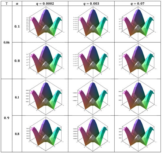
Figure 1. The absolute error comparison at $\mathit{T}=\mathbf{0.06},\mathit{t}=\mathbf{0.9}$ for $\mathit{\alpha }=\mathbf{0.1}$, $\mathit{\alpha }=\mathbf{0.8},$ according to $\mathit{q}=\mathbf{0.0002},\mathbf{0.003},\mathbf{0.07}$.

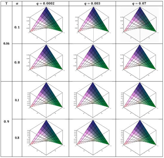
Figure 2. The numerical solution at $\mathit{T}=\mathbf{0.06},\mathit{t}=\mathbf{0.9}$ for $\mathit{\alpha }=\mathbf{0.1}$, $\mathit{\alpha }=\mathbf{0.8},$ when $\mathit{q}=\mathbf{0.0002},\mathbf{0.003},\mathbf{0.07}$.

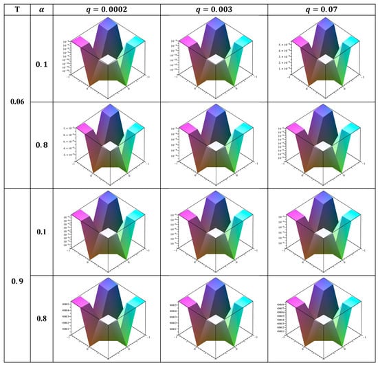
Figure 3. The comparison of absolute error values for the Carleman parameter $\omega =\mathbf{0.35}$, at $\mathit{T}=\mathbf{0.06}, \mathbf{0.9},$ where the fractional derivative takes the values $\mathit{\alpha }=\mathbf{0.1}, \mathrm{and} \mathbf{0.8}$.

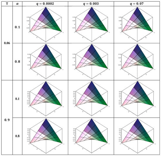
Figure 4. The approximate solution at $\mathit{T}=\mathbf{0.06},\mathit{t}=\mathbf{0.9}$ for $\omega =\mathbf{0.35}$, where $\mathit{\alpha }=\mathbf{0.1}, \mathrm{and} \mathbf{0.8}$.

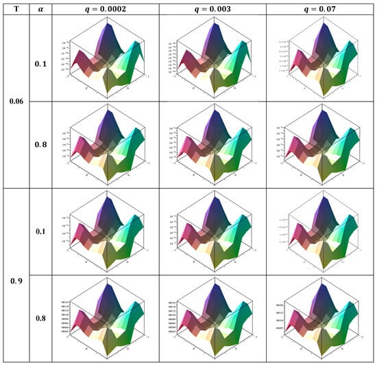
Figure 5. The absolute error values at $\mathit{T}=\mathbf{0.06}$, $\mathbf{0.9}$, for the fractional derivative order $\mathit{\alpha }=\mathbf{0.2} \mathrm{and} \mathbf{0.8}$.

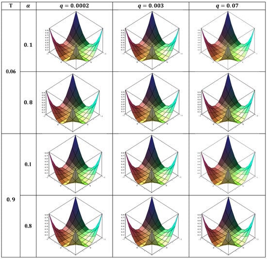
Figure 6. The numerical solution for the fractional derivative order $\mathit{\alpha }=\mathbf{0.2}, \mathbf{0.8}$, at $\mathit{T}=\mathbf{0.06}$, $\mathbf{0.9}$.

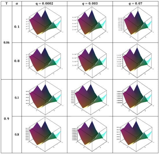
Figure 7. A comparison of the absolute error values for the Carleman parameter $\omega =\mathbf{0.35}$, at $\mathit{T}=\mathbf{0.06},\mathbf{0.09}$, where $\mathit{\alpha }=\mathbf{0.1}, \mathbf{0.8}$ represent the fractional derivative order.

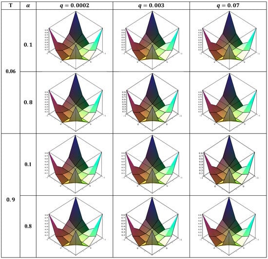
Figure 8. The numerical solution $\omega =\mathbf{0.35},$ at $\mathit{T}=\mathbf{0.06}$, $\mathbf{0.9}$, where the fractional derivative order $\mathit{\alpha }=\mathbf{0.1}, \mathbf{0.8}$.

Application 1: Logarithmic kernel:

The importance of logarithmic kernel in mixed integral equation can be found in the work of Alhazmi et al. [1]

Consider the phase-lag (2 + 1) DMIE equation

$$\mathsf{\Phi }\left(u,v;t-q\right)=f\left(u,v;t\right)+\lambda {\int }_0^t{\int }_{-1}^1{\int }_{-1}^1\left(t^2+\tau \right) \ln \left|u-\delta \right|\ln \left|v-\gamma \right|\mathsf{\Phi }\left(\delta ,\gamma ;\tau \right)d\delta d\gamma d\tau ,$$

(57)

with conditions

$$\mathsf{\Phi }\left(u,v;0\right)={\displaystyle \frac{uv}{10}} , {\left.{\displaystyle \frac{\partial \mathsf{\Phi }\left(u,v;t\right)}{\partial t}}\right]}_{t=0}=0.$$

(58)

Equation (57) can be rewritten with the aid of (58) in the form a MIE in (2 + 1) dimension

$$\begin{gathered} {\displaystyle \frac{q^{\alpha +1}}{\mathsf{\Gamma }\left(\alpha +2\right)}}\left[\mathsf{\Phi }\left(u,v;t\right)-{\displaystyle \frac{\left(\alpha +1\right)}{q}}{\int }_0^t\left(1-{\displaystyle \frac{\alpha {\left(t-\tau \right)}^{\alpha }}{q^{\alpha }}}\right)\mathsf{\Phi }\left(u,v;\tau \right)d\tau \right. \\ -{\displaystyle \frac{\lambda \alpha \left(\alpha +1\right)}{2 }}{\int }_0^t{\left(t-\tau \right)}^{\alpha +1}\left(t^2+\tau \right)d\tau \left.{\int }_c^d\ln \left|v-\gamma \right|{\int }_a^b\ln \left|u-\delta \right|\mathsf{\Phi }\left(\delta ,\gamma ;\tau \right)d\delta d\gamma \right] \\ ={\displaystyle \frac{1}{\mathsf{\Gamma }\left(\alpha \right) }}{\int }_0^t{\left(t-\tau \right)}^{\alpha }f\left(u,v;\tau \right)d\tau +{\displaystyle \frac{q^{\alpha +1}}{\mathsf{\Gamma }\left(\alpha +2\right)}}\left({\displaystyle \frac{uv}{10}}\right). \end{gathered}$$

(59)

The exact solution is $\mathsf{\Phi }\left(u,v;t\right)=uv(t^3+0.1)$, $U\left(t\right)=\left(t^3+0.1\right)$.

Table 3 and Table 4 indicate that the accuracies of the numerical solution of Equation (59) are ${10}^{-7}$ for $\mathsf{\alpha }=0.1$ and ${10}^{-6}$ for $\mathsf{\alpha }=0.8$ when T = 0.06; ${10}^{-4}$ for $\mathsf{\alpha }=0.1$ and ${10}^{-3}$ for $\mathsf{\alpha }=0.8$ when T = 0.9.

Table 3. Shows the numerical solutions for T = 0.06 along with the associated errors.

α	(x, y)	q = 0.0002		q = 0.003		q = 0.07
		Num. Sol.	Error	Num. Sol.	Error	Num. Sol.	Error
0.1	(±1, ±1)	±0.100216007	6.9774 × 10−9	±0.100216005	5.34990 × 10−9	±0.100215979	2.13073 × 10−8
	(±0.5, ±1) (±1, ±0.5)	±0.05010801	6.3372 × 10−9	±0.05010801	4.87618 × 10−9	±0.05010798	1.94338 × 10−8
	(0.0, ±1) (±1, 0.0)	±1.15 × 10−20	1.1464 × 10−20	±6.74 × 10−21	6.7399 × 10−21	±8.62 × 10−21	8.6201 × 10−21
	(0.0, ±0.5) (±0.5, 0.0)	±5.73 × 10−21	5.7321 × 10−21	±3.37 × 10−21	3.3699 × 10−21	±4.31 × 10−21	4.3101 × 10−21
	(±0.5, ±0.5)	±0.025054006	5.78279 × 10−9	±0.025054004	4.44250 × 10−9	±0.025053982	1.77307 × 10−8
0.8	(±1, ±1)	±0.100215962	3.83557 × 10−8	±0.100215953	4.67728 × 10−8	±0.100215649	3.50759 × 10−7
	(±0.5, ±1) (±1, ±0.5)	±0.05010796	3.49964 × 10−8	±0.05010796	5.50074 × 10−8	±0.05010768	3.19868 × 10−7
	(0.0, ±1) (±1, 0.0)	±3.51 × 10−21	3.5096 × 10−21	±5.22 × 10−21	5.2189 × 10−21	±3.21 × 10−19	3.2053 × 10−19
	(0.0, ±0.5) (±0.5, 0.0)	±1.75 × 10−21	1.7548 × 10−21	±2.61 × 10−21	2.6095 × 10−21	±1.60 × 10−19	1.6026 × 10−19
	(±0.5, ±0.5)	±0250539681	3.19071 × 10−8	±0.02505396	5.01720 × 10−8	±0.025053708	2.91713 × 10−8

Table 4. Provides the approximate solution for T = 0.9 together with the related error.

α	(x, y)	q = 0.0002		q = 0.003		q = 0.07
		Num. Sol.	Error	Num. Sol.	Error	Num. Sol.	Error
0.1	(±1, ±1) (−1, −1)	±0.829037206	3.72063 × 10−5	±0.829027082	2.70817 × 10−5	±0.829024343	2.43433 × 10−5
	(±0.5, ±1) (±1, ±0.5)	±0.41453393	3.39313 × 10−5	±0.41452469	2.46979 × 10−5	±0.41452220	2.22005 × 10−5
	(0.0, ±1) (±1, 0.0)	±6.24 × 10−18	6.2399 × 10−18	±3.31 × 10−18	3.3059 × 10−18	±2.67 × 10−18	2.6711 × 10−18
	(0.0, ±0.5) (±0.5, 0.0)	±3.12 × 10−18	3.1202 × 10−18	±1.65 × 10−18	1.6530 × 10−18	±1.34 × 10−18	1.3356 × 10−18
	(±0.5, ±0.5)	±0.207280945	3.09447 × 10−5	±0.207272524	2.25239 × 10−5	±0.207270246	2.02464 × 10−5
0.8	(±1, ±1)	±0.828792380	2.07620 × 10−4	±0.828785621	2.14379 × 10−4	±0.828662607	3.37393 × 10−4
	(±0.5, ±1) (±1, ±0.5)	±0.41431065	1.89345 × 10−4	±0.41430449	1.95510 × 10−4	±0.41419230	3.07696 × 10−4
	(0.0, ±1) (±1, 0.0)	±1.25 × 10−18	1.2482 × 10−18	±.1.65 × 10−18	1.6530 × 10−18	±3.30 × 10−18	3.2966 × 10−18
	(0.0, ±0.5) (±0.5, 0.0)	±6.24 × 10−19	6.2410 × 10−19	±6.66 × 10−19	6.6558 × 10−19	±1.65 × 10−18	1.6483 × 10−18
	(±0.5, ±0.5)	±0.207077321	1.72679 × 10−4	±0.207071699	1.78301 × 10−4	±0.206969388	2.80612 × 10−4

Recalling that the function $\mathsf{\Phi }$ and hence the approximate solution is logically positive when both $u$ and $v$ are either positive or negative, and negative when one is positive and the other is negative.

Application 2: Carleman kernel:

Carleman kernel has many application in the theory of singular integral equations, see Jan [4] and Raad and Al-Atawi [19].

Consider the phase-lag (2 + 1) dimension MIE equation

$$\mathsf{\Phi }\left(u,v;t-q\right)=f\left(u,v;t\right)+\lambda {\int }_0^t{\int }_c^d{\int }_a^b\left(t^2+\tau \right) {\left|u-\delta \right|}^{-\omega }{\left|v-\gamma \right|}^{-\omega }\mathsf{\Phi }\left(\delta ,\gamma ;\tau \right)d\delta d\gamma d\tau . (0\le \omega <1)$$

(60)

Equation (60) can be rewritten with the aid of (58) in the form a MIE in (2 + 1) dimension

$$\begin{gathered} {\displaystyle \frac{q^{\alpha +1}}{\mathsf{\Gamma }\left(\alpha +2\right)}}\left[\mathsf{\Phi }\left(u,v;t\right)-{\displaystyle \frac{\left(\alpha +1\right)}{q}}{\int }_0^t\left(1-{\displaystyle \frac{\alpha {\left(t-\tau \right)}^{\alpha }}{q^{\alpha }}}\right)\mathsf{\Phi }\left(u,v;\tau \right)d\tau \right.-{\displaystyle \frac{\lambda \alpha \left(\alpha +1\right)}{2 }} \\ \left.\times {\int }_0^t{\left(t-\tau \right)}^{\alpha +1}\left(t^2+\tau \right)d\tau {\int }_c^d{\left|v-\gamma \right|}^{-\omega }{\int }_a^b{\left|u-\delta \right|}^{-\omega }\mathsf{\Phi }\left(\delta ,\gamma ;\tau \right)d\delta d\gamma \right] \\ ={\displaystyle \frac{1}{\mathsf{\Gamma }\left(\alpha \right) }}{\int }_0^t{\left(t-\tau \right)}^{\alpha }f\left(u,v;\tau \right)d\tau +{\displaystyle \frac{q^{\alpha +1}}{\mathsf{\Gamma }\left(\alpha +2\right)}}\left({\displaystyle \frac{uv}{10}}\right). \end{gathered}$$

(61)

The exact solution is $\mathsf{\Phi }\left(u,v;t\right)=uv(t^3+0.1)$, $U\left(t\right)=\left(t^3+0.1\right)$.

The approximate solution of Equation (61) has the following accuracy values ${10}^{-8}$ for $\mathsf{\alpha }=0.1$ and ${10}^{-7}$ for $\mathsf{\alpha }=0.8$ when T = 0.06; ${10}^{-4}$ for $\mathsf{\alpha }=0.$ 8 and ${10}^{-5}$ for $\mathsf{\alpha }=0.1$ when T = 0.9. These values are shown in Table 5 and Table 6. Note that if both $u$ and $v$ are positive or negative, the function Φ and, consequently, the approximate solution, are logically positive; if one is positive and the other is negative, the function is logically negative.

Table 5. Shows the numerical solutions for T = 0.06 along alongside the related error.

α	(x, y)	q = 0.0002		q = 0.003		q = 0.07
		Num. Sol.	Error	Num. Sol.	Error	Num. Sol.	Error
0.1	(±1, ±1)	±0.100216002	1.8093 × 10−9	±0.100216001	1.3873 × 10−9	±0.100215994	5.5875 × 10−9
	(±0.5, ±1) (±1, ±0.5)	±0.05010800	1.7763 × 10−9	±0.05010800	1.3791 × 10−9	±0.05010799	5.4727 × 10−9
	(0.0, ±1) (±1, 0.0)	±1.09 × 10−18	1.094 × 10−18	±6.43 × 10−19	6.429 × 10−19	±1.32 × 10−18	1.318 × 10−18
	(0.0, ±0.5) (±0.5, 0.0)	±5.47 × 10−18	5.468 × 10−18	±3.21 × 10−19	3.215 × 10−19	±6.59 × 10−19	6.588 × 10−19
	(±0.5, ±0.5)	±0.025054002	1.7447 × 10−9	±0.025054001	1.3463 × 10−9	±0.025053995	5.3689 × 10−9
0.8	(±1, ±1)	±0.100215990	1.0073 × 10−8	±0.100215988	1.2283 × 10−8	±0.100215908	9.1971 × 10−8
	(±0.5, ±1) (±1, ±0.5)	±0.05010799	9.8341 × 10−9	±0.05010799	1.1992 × 10−8	±0.05010791	9.0024 × 10−8
	(0.0, ±1) (±1, 0.0)	±5.53 × 10−18	5.528 × 10−18	±8.22 × 10−18	8.220 × 10−18	±5.24 × 10−17	5.237 × 10−17
	(0.0, ±0.5) (±0.5, 0.0)	±2.76 × 10−18	2.7639 × 10−18	±4.11 × 10−18	4.110 × 10−18	±2.62 × 10−17	2.6186 × 10−17
	(±0.5, ±0.5)	±0.025053990	9.6324 × 10−9	±0.025053988	1.1746 × 10−8	±0.025053912	8.8136 × 10−8

Table 6. Provides the approximate solution at T = 0.7 together with the corresponding error.

α	(x, y)	q = 0.0002		q = 0.003		q = 0.07
		Num. Sol.	Error	Num. Sol.	Error	Num. Sol.	Error
0.1	(±1, ±1)	±0.829009757	9.7566 × 10−6	±0.829007102	7.1017 × 10−6	±0.829006384	6.3836 × 10−6
	(±0.5, ±1) (±1, ±0.5)	±0.41450955	9.5511 × 10−6	±0.41450695	6.9521 × 10−6	±0.41450625	6.2491 × 10−6
	(0.0, ±1) (±1, 0.0)	±1.11 × 10−15	1.105 × 10−15	±5.85 × 10−16	5.852 × 10−16	±4.73 × 10−16	4.729 × 10−16
	(0.0, ±0.5) (±0.5, 0.0)	±5.52 × 10−15	5.523 × 10−15	±2.93 × 10−16	2.926 × 10−16	±2.36 × 10−16	2.364 × 10−16
	(±0.5, ±0.5)	±0.207259350	9.3499 × 10−6	±0.207256806	6.8056 × 10−6	±0.207256117	6.1174 × 10−6
0.8	(±1, ±1)	±0.828945556	5.4444 × 10−5	±0.828943784	5.6216 × 10−5	±0.828911526	8.8474 × 10−5
	(±0.5, ±1) (±1, ±0.5)	±0.41444670	5.3297 × 10−5	±0.41444497	5.5032 × 10−5	±0.41441389	8.6611 × 10−5
	(0.0, ±1) (±1, 0.0)	±5.20 × 10−16	5.196 × 10−16	±5.54 × 10−16	5.539 × 10−16	±1.37 × 10−15	1.371 × 10−15
	(0.0, ±0.5) (±0.5, 0.0)	±2.60 × 10−16	2.598 × 10−16	±2.77 × 10−16	2.769 × 10−16	±6.86 × 10−16	6.856 × 10−16
	(±0.5, ±0.5)	±0.207197825	5.2175 × 10−5	±0.207196127	5.3873 × 10−5	±0.207165214	8.4786 × 10−6

Application (3): Logarithmic kernel:

For the double logarithmic kernel in two-dimensional, see Jan et al. [14]

Consider the phase-lag (2 + 1) DMIE equation

$$\mathsf{\Phi }\left(u,v;t-q\right)=f\left(u,v;t\right)+{\displaystyle \frac{1}{2}}{\int }_0^t{\int }_c^d{\int }_a^b\left(t. \tau \right) \ln \left|u-\delta \right|\ln \left|v-\gamma \right|\mathsf{\Phi }\left(\delta ,\gamma ;\tau \right)d\delta d\gamma d\tau ,$$

(62)

with conditions

$$\mathsf{\Phi }\left(u,v,0\right)=u^2{v}^2 , {\left.{\displaystyle \frac{\partial \mathsf{\Phi }\left(u,v,t\right)}{\partial t}}\right]}_{t=0}=-{\displaystyle \frac{u^2 v^2}{5}}.$$

(63)

Equation (62) can be rewritten with the aid of (63) in the form

$$\begin{gathered} {\displaystyle \frac{q^{\alpha +1}}{\mathsf{\Gamma }\left(\alpha +2\right)}}\left[\mathsf{\Phi }\left(u,v;t\right)-{\displaystyle \frac{\left(\alpha +1\right)}{q}}{\int }_0^t\left(1-{\displaystyle \frac{\alpha {\left(t-\tau \right)}^{\alpha }}{q^{\alpha }}}\right)\mathsf{\Phi }\left(u,v;\tau \right)d\tau \right.-{\displaystyle \frac{\lambda \alpha \left(\alpha +1\right)}{2 }} \\ \left.\times {\int }_0^t{\left(t-\tau \right)}^{\alpha +1}\left(t. \tau \right) d\tau {\int }_c^d\ln \left|v-\gamma \right|{\int }_a^b\ln \left|u-\delta \right|\mathsf{\Phi }\left(\delta ,\gamma ;\tau \right)d\delta d\gamma \right] \\ ={\displaystyle \frac{1}{\mathsf{\Gamma }\left(\alpha \right) }}{\int }_0^t{\left(t-\tau \right)}^{\alpha }f\left(u,v;\tau \right)d\tau +{\displaystyle \frac{q^{\alpha +1}{u}^2 v^2}{\mathsf{\Gamma }\left(\alpha +2\right)}}\left(1-{\displaystyle \frac{t^{\alpha }}{5\mathsf{\Gamma }\left(\alpha +1\right)}}\right) . \end{gathered}$$

(64)

The exact solution is $\mathsf{\Phi }\left(u,v;t\right)=u^2{v}^2{e}^{-t/5}$, $U\left(t\right)=e^{-t/5}.$

The numerical solution of Equation (64) has accuracy values of ${10}^{-7}$ for $\mathsf{\alpha }=0.1$ and ${10}^{-6}$ for $\mathsf{\alpha }=0.8$ when T = 0.06; ${10}^{-3}$ for $\mathsf{\alpha }=0.$ 8 and ${10}^{-4}$ for $\mathsf{\alpha }=0.1$ when T = 0.9, as indicated by Table 7 and Table 8.

Table 7. Shows the approximate solutions for T = 0.06 along with the associated errors.

α	(x, y)	q = 0.0002		q = 0.003		q = 0.07
		Num. Sol.	Error	Num. Sol.	Error	Num. Sol.	Error
0.1	(±1, ±1)	0.988071714	1.958 × 10−10	0.988071713	1.501 × 10	0.988071713	3.513 × 10−10
	(±0.5, ±1) (±1, ±0.5)	0.247017928	2.678 × 10−10	0.247017928	1.501 × 10−10	0.247017927	7.609 × 10−10
	(0.0, ±1) (±1, 0.0)	7.381 × 10−11	7.381 × 10−11	5.65697 × 10−11	5.657 × 10−11	2.389 × 10−10	2.389 × 10−10
	(0.0, ±0.5) (±0.5, 0.0)	2.746 × 10−10	2.746 × 10−10	2.10452× 10−10	2.105 × 10−10	8.888 × 10−10	8.888 × 10−10
	(±0.5, ±0.5)	0.061754483	5.471 × 10−10	0.061754482	4.082 × 10−10	0.061754480	1.8292 × 10−9
	(0.0, 0.0)	1.713 × 10−10	1.713 × 10−10	1.31276 × 10−10	1.313 × 10−10	5.544 × 10−10	5.544 × 10−10
0.8	(±1, ±1)	0.988071714	7.042 × 10−10	0.988071714	8.342 × 10−10	0.988071719	5.8033 × 10−9
	(±0.5, ±1) (±1, ±0.5)	0.247017927	7.0422 × 10−9	0.247017927	1.5562 × 10−9	0.247017916	1.2444 × 10−8
	(0.0, ±1) (±1, 0.0)	3.931 × 10−10	3.931 × 10−10	4.79153 × 10−10	4.791 × 10−10	3.9947 × 10−9	3.9947 × 10−9
	(0.0, ±0.5) (±0.5, 0.0)	1.4623 × 10−9	1.4623 × 10−9	1.782555 × 10−9	1.7826 × 10−9	1.4861 × 10−8	1.4861 × 10−8
	(±0.5, ±0.5)	0.061754479	2.9951 × 10−9	0.061754478	3.6777 × 10−9	0.061754452	3.0483 × 10−8
	(0.0, 0.0)	9.122 × 10−10	9.122 × 10−10	1.111926 × 10−9	1.1119 × 10−9	9.2701 × 10−9	9.2701 × 10−9

Table 8. Provides the numerical solution for T = 0.9 along with the related error.

α	(x, y)	q = 0.0002		q = 0.003		q = 0.07
		Num. Sol.	Error	Num. Sol.	Error	Num. Sol.	Error
0.1	(±1, ±1)	0.835269777	4.3446 × 10−7	0.835269899	3.1250 × 10−7	0.835269978	2.3311 × 10−7
	(±0.5, ±1) (±1, ±0.5)	0.208818468	9.1511 × 10−7	0.208818211	6.5817 × 10−7	0.208818044	4.9093 × 10−7
	(0.0, ±1) (±1, 0.0)	2.9334 × 10−7	2.9334 × 10−7	2.1099 × 10−7	2.1099 × 10−7	1.5740 × 10−7	1.5740 × 10−7
	(0.0, ±0.5) (±0.5, 0.0)	1.0913 × 10−6	1.0913 × 10−6	7.8494 × 10−7	7.8494 × 10−7	5.8555 × 10−7	5.8555 × 10−7
	(±0.5, ±0.5)	0.052206628	2.2398 × 10−6	0.052205999	1.6110 × 10−6	0.052205590	1.2018 × 10−6
	(0.0, 0.0)	6.8072 × 10−7	6.8072 × 10−7	4.8963 × 10−7	4.8963 × 10−7	3.6526 × 10−7	3.6526 × 10−7
0.8	(±1, ±1)	0.835271821	1.6095 × 10−6	0.835271854	1.6428 × 10−6	0.835272420	2.2084 × 10−6
	(±0.5, ±1) (±1, ±0.5)	0.208814162	3.3906 × 10−6	0.208814092	3.4608 × 10−6	0.208812900	4.6524 × 10−6
	(0.0, ±1) (±1, 0.0)	1.0869 × 10−6	1.0869 × 10−6	1.1094 × 10−6	1.1094 × 10−6	1.4915 × 10−6	1.4915 × 10−6
	(0.0, ±0.5) (±0.5, 0.0)	4.0436 × 10−6	4.0436 × 10−6	4.1273 × 10−6	4.1273 × 10−6	5.5486 × 10−6	5.5486 × 10−6
	(±0.5, ±0.5)	0.052196089	8.2990 × 10−5	0.052195917	8.4708 × 10−6	0.052193000	1.1388 × 10−5
	(0.0, 0.0)	2.5223 × 10−6	2.5223 × 10−6	2.5745 × 10−6	2.5745 × 10−6	3.4611 × 10−6	3.4611 × 10−6

Application 4: Carleman kernel:

For the double Carleman kernel in two-dimensional see Jan et al. [14]

Consider the phase-lag (2 + 1)D-MIE equation

$$\mathsf{\Phi }\left(u,v;t-q\right)=f\left(u,v;t\right)+{\displaystyle \frac{1}{2}}{\int }_0^t{\int }_c^d{\int }_a^b\left(t. \tau \right) {\left|u-\delta \right|}^{-\omega }{\left|v-\gamma \right|}^{-\omega }\mathsf{\Phi }\left(\delta ,\gamma ;\tau \right)d\delta d\gamma d\tau .$$

(65)

Equation (65) can be rewritten with the aid of (63) in the form

$$\begin{gathered} {\displaystyle \frac{q^{\alpha +1}}{\mathsf{\Gamma }\left(\alpha +2\right)}}\left[\mathsf{\Phi }\left(u,v;t\right)-{\displaystyle \frac{\left(\alpha +1\right)}{q}}{\int }_0^t\left(1-{\displaystyle \frac{\alpha {\left(t-\tau \right)}^{\alpha }}{q^{\alpha }}}\right)\mathsf{\Phi }\left(u,v;\tau \right)d\tau \right.-{\displaystyle \frac{\lambda \alpha \left(\alpha +1\right)}{2 }} \\ \left.\times {\int }_0^t{\left(t-\tau \right)}^{\alpha +1}\left(t. \tau \right) d\tau {\int }_c^d{\left|v-\gamma \right|}^{-\omega }{\int }_a^b{\left|u-\delta \right|}^{-\omega }\mathsf{\Phi }\left(\delta ,\gamma ;\tau \right)d\delta d\gamma \right] \\ ={\displaystyle \frac{1}{\mathsf{\Gamma }\left(\alpha \right) }}{\int }_0^t{\left(t-\tau \right)}^{\alpha }f\left(u,v;\tau \right)d\tau +{\displaystyle \frac{q^{\alpha +1}{u}^2 v^2}{\mathsf{\Gamma }\left(\alpha +2\right)}}\left(1-{\displaystyle \frac{t^{\alpha }}{5\mathsf{\Gamma }\left(\alpha +1\right)}}\right). \end{gathered}$$

(66)

The exact solution is $\mathsf{\Phi }\left(u,v;t\right)=u^2{v}^2{e}^{-t/5}$, $U\left(t\right)=e^{-t/5}.$

The following accuracy values are associated with the approximate solution of Equation (66): ${10}^{-5}$ for $\mathsf{\alpha }=0.8$ and ${10}^{-6}$ for $\mathsf{\alpha }=0.1$ when T = 0.06; ${10}^{-3}$ when T = 0.9, Table 9 and Table 10 present these values.

Table 9. Shows the numerical solutions for t = 0.06 together with the corresponding error.

α	(x, y)	q = 0.0002		q = 0.003		q = 0.07
		Num. Sol.	Error	Num. Sol.	Error	Num. Sol.	Error
0.1	(±1, ±1)	0.988071720	6.7307 × 10−9	0.988071718	5.1587 × 10−9	0.988071691	2.1927 × 10−8
	(±0.5, ±1) (±1, ±0.5)	0.247017935	6.8470 × 10−9	0.247017933	5.2369 × 10−9	0.247017906	2.1950 × 10−8
	(0.0, ±1) (±1, 0.0)	7.9725 × 10−9	7.9725 × 10−9	6.1104 × 10−9	6.1104 × 10−9	2.5805 × 10−8	2.5805 × 10−8
	(0.0, ±0.5) (±0.5, 0.0)	3.7631 × 10−9	3.7631 × 10−9	2.8842 × 10−9	2.8842 × 10−9	1.2180 × 10−8	1.2180 × 10−8
	(±0.5, ±0.5)	0.061754486	3.8397 × 10−9	0.061754485	2.9318 × 10−9	0.061754470	1.2474 × 10−8
	(0.0, 0.0)	1.9756 × 10−9	1.9756 × 10−9	1.5142 × 10−9	1.5142 × 10−9	6.3946 × 10−9	6.3946 × 10−9
0.8	(±1, ±1)	0.988071677	3.5915 × 10−8	0.988071669	4.3780 × 10−8	0.988071347	3.6567 × 10−7
	(±0.5, ±1) (±1, ±0.5)	0.247017892	3.5980 × 10−8	0.247017884	4.3843 × 10−8	0.247017562	3.6604 × 10−7
	(0.0, ±1) (±1, 0.0)	4.2459 × 10−8	4.2459 × 10−8	5.1756 × 10−8	5.1756 × 10−8	4.3149 × 10−7	4.3149 × 10−7
	(0.0, ±0.5) (±0.5, 0.0)	2.0041 × 10−8	2.0041 × 10−8	2.4429 × 10−8	2.4429 × 10−8	2.0367 × 10−7	2.0367 × 10−7
	(±0.5, ±0.5)	0.061754462	2.0464 × 10−8	0.061754457	2.4972 × 10−8	0.061754274	2.0837 × 10−7
	(0.0, 0.0)	1.0521 × 10−8	1.0521 × 10−8	1.2825 × 10−8	1.2825 × 10−8	1.0692 × 10−7	1.0692 × 10−7

Table 10. Shows the numerical solutions for T = 0.9 along with the associated errors.

α	(x, y)	q = 0.0002		q = 0.003		q = 0.07
		Num. Sol.	Error	Num. Sol.	Error	Num. Sol.	Error
0.1	(±1, ±1)	0.835297081	2.6870 × 10−5	0.835289538	1.9327 × 10−5	0.835284629	1.4417 × 10−5
	(±0.5, ±1) (±1, ±0.5)	0.208844433	2.6880 × 10−5	0.208836887	1.9334 × 10−5	0.208831976	1.4423 × 10−5
	(0.0, ±1) (±1, 0.0)	3.1687 × 10−5	3.1687 × 10−5	2.2791 × 10−5	2.2791 × 10−5	1.7002 × 10−5	1.7002 × 10−5
	(0.0, ±0.5) (±0.5, 0.0)	1.4956 × 10−5	1.4956 × 10−5	1.0758 × 10−5	1.0758 × 10−5	8.0250 × 10−6	8.0250 × 10−6
	(±0.5, ±0.5)	0.052219691	1.5303 × 10−5	0.052215395	1.1007 × 10−5	0.052212599	8.2108 × 10−5
	(0.0, 0.0)	7.8521 × 10−6	7.8521 × 10−6	5.6478 × 10−6	5.6478 × 10−6	4.2131 × 10−6	4.2131 × 10−6
0.8	(±1, ±1)	0.835170662	9.9549 × 10−5	0.835168602	1.0161 × 10−4	0.835133616	1.3660 × 10−4
	(±0.5, ±1) (±1, ±0.5)	0.208717965	9.9587 × 10−5	0.208715905	1.0165 × 10−4	0.208680905	1.3665 × 10−4
	(0.0, ±1) (±1, 0.0)	1.1739 × 10−4	1.1739 × 10−4	1.1982 × 10−4	1.1982 × 10−4	1.6107 × 10−4	1.6107 × 10−4
	(0.0, ±0.5) (±0.5, 0.0)	5.5406 × 10−5	5.5406 × 10−5	5.6553 × 10−5	5.6553 × 10−5	7.6023 × 10−5	7.6023 × 10−5
	(±0.5, ±0.5)	0.052147694	5.6694 × 10−5	0.052146521	5.786723E-5	0.052126596	7.7792 × 10−5
	(0.0, 0.0)	2.9088 × 10−5	2.9088 × 10−5	2.9689 × 10−5	2.9689 × 10−5	3.9911 × 10−5	3.9911 × 10−5

11. Discussion

From the previous results and figures, it can be concluded that:

(1)

It is apparent that the inaccuracy grows over time, and this makes sense.

(2)

Cases where $u=0$ or $v=0$ in applications (1 and 2) all have zero solutions, which is why they are not included in the tables.

(3)

The numerical solution is a good approximation of the exact solution, as shown by the extremely small error values.

(4)

There seems to be minimal impact on the error values when the fractional power α is altered.

(5)

The results presented in the previous tables show how the phase lag’s effect grows over an extended amount of time.

(6)

According to the logarithmic kernel results, Application 3’s accuracy is nearly equivalent to that of Application 1.

(7)

Application 2 performs better than Application 4 in terms of the Carleman kernel’s results accuracy, indicating that results are impacted by the time function’s status as an exponential function compared to the polynomial.

(8)

The numerical results maintain the symmetric property of the exact solution for both variables, $u$ and $v$.

(9)

The graphs 1–8 verified the effectiveness of the suggested methods.

12. Conclusions

In this study we can established the following:

(1)

We focused on studying the P-MIE with singular kernels, which has tremendous value in mathematical modeling. After using Taylor’s expansion and then using Riemann-Liouville fractional integral on P-MIE, a MIE in (2 + 1) dimensions in position and time was obtained.

(2)

The convergence of the MIE solution was demonstrated by showing that the infinite series of solutions converges uniformly to a continuous function.

(3)

The contraction theorem has been used to prove that a solution exists and is unique under certain conditions by proving that the integral operator is bounded and continuous. Error estimation was discussed to prove the convergence of the error and thus the approximate solution.

(4)

The separation of variables method is a powerful scheme that allows us to transform a multidimensional MIE that depends on time variable into a set of two-dimensional integral equations in position with time-dependent coefficients.

(5)

The connection between position kernels and time-dependent coefficients is investigated. The Nystrӧm method, as an effective numerical method, was applied to the resulting integral equation to achieve a system of linear algebraic equations, which can be easily solved numerically.

(6)

PNM was applied to MIE with logarithmic kernel and Carleman function as popular types of singular kernel. Numerical calculations were performed by using Maple 18. The computational results show how effective and applicable the strategies used to solve P-MIE were.

13. Future Work

We will use the Toeplitz matrix approach to examine the identical issue in the nonlinear situation, and we will compare the Toeplitz matrix method with the product Nystrom method in the nonlinear case.

References

- Alhazmi, S.E.; Abdou, M.A.; Basseem, M. Physical phenomena of spectral relationships via quadratic third kind mixed integral equation with discontinuous kernel. AIMS Math. 2023, 8, 24379–24400. [Google Scholar] [CrossRef]
- Basseem, M.; Alalyani, A. On the solution of quadratic nonlinear integral equation with different singular kernels. Math. Probl. Eng. 2020, 1, 7856207. [Google Scholar] [CrossRef]
- Afiatdoust, F.; Heydari, M.H.; Hosseini, M.M. A block-by-block method for nonlinear variable-order fractional quadratic integral equations. Comput. Appl. Math. 2023, 42, 1–38. [Google Scholar] [CrossRef]
- Jan, A.R. An asymptotic model for solving mixed integral equation in position and time. J. Math. 2022, 2022, 8063971. [Google Scholar] [CrossRef]
- Sur, A.; Paul, S.; Kanoria, M. Modeling of memory-dependent derivative in a functionally graded plate. Waves Random Complex Media 2021, 31, 618–638. [Google Scholar] [CrossRef]
- Chiriţă, S. On the time differential dual-phase-lag thermoelastic model. Meccanica 2017, 52, 349–361. [Google Scholar] [CrossRef]
- Farengo, R.; Lee, Y.C.; Guzdar, P.N. An electromagnetic integral equation: Application to microtearing modes. Phys. Fluids 1983, 26, 3515–3523. [Google Scholar] [CrossRef]
- Abdou, M.A.; Nasr, M.E.; Abdel-Aty, M.A. Study of the normality and continuity for the mixed integral equations with phase-lag term. Int. J. Math. Anal. 2017, 11, 787–799. [Google Scholar] [CrossRef]
- Aljawi, S.; Aljohani, S.; Kamran; Ahmed, A.; Mlaiki, N. Numerical Solution of the Linear Fractional Delay Differential Equation Using Gauss–Hermite Quadrature. Symmetry 2024, 16, 721. [Google Scholar] [CrossRef]
- Rostami, Y.; Maleknejad, K. A novel approach to solving system of integral partial differential equations based on hybrid modified block-pulse functions. Math. Methods Appl. Sci. 2024, 47, 5798–5818. [Google Scholar] [CrossRef]
- Nili Ahmadabadi, M. An efficient method for mixed integral equations with phase lag. Int. J. Comput. Math. 2020, 97, 1170–1182. [Google Scholar] [CrossRef]
- Mosa, G.A.; Abdou, M.A.; Rahby, A.S. Numerical solutions for nonlinear Volterra-Fredholm integral equations of the second kind with a phase lag. AIMS Math 2021, 6, 8525–8543. [Google Scholar] [CrossRef]
- Jan, A.R.; Abdou, M.A.; Basseem, B. A Physical Phenomenon for the Fractional Nonlinear Mixed Integro-Differential Equation Using a Quadrature Nystrom Method. Fractal Fract. 2023, 7, 656. [Google Scholar] [CrossRef]
- Xie, J. Numerical computation of fractional partial differential equations with variable coefficients utilizing the modified fractional Legendre wavelets and error analysis. Math. Methods Appl. Sci. 2021, 44, 7150–7164. [Google Scholar] [CrossRef]
- Chandler-Wilde, S.N.; Gover, M.J.C. On the application of a generalization of Toeplitz matrices to the numerical solution of integral equations with weakly singular convolution kernels. J. Numer. Anal. IMAJNA 1989, 9, 525–544. [Google Scholar] [CrossRef]
- Golberg, M.A. Introduction to the numerical solution of Cauchy singular integral equations. In Numerical Solution of Integral Equations; Springer: Berlin/Heidelberg, Germany, 1990; pp. 183–308. [Google Scholar]
- Shpazzadeh, E.; Chu, Y.M.; Hashemi, M.S.; Moharrami, M.; Inc, M. Hermite multiwavelets representation for the sparse solution of nonlinear Abel’s integral equation. Appl. Math. Comput. 2022, 427, 127171. [Google Scholar] [CrossRef]
- Assari, P.; Adibi, H.; Dehghan, M. The numerical solution of weakly singular integral equations based on the meshless product integration (MPI) method with error analysis. Appl. Numer. Math. 2014, 81, 76–93. [Google Scholar] [CrossRef]
- Theocaris, P.S. Numerical solution of singular integral equations: Methods. J. Eng. Mech. Div. 1981, 107, 733–752. [Google Scholar] [CrossRef]
- Raad, S.A.; Abdou, M.A. An Algorithm for the Solution of Integro-Fractional Differential Equations with a Generalized Symmetric Singular Kernel. Fractal Fract. 2024, 8, 644. [Google Scholar] [CrossRef]
- Raad, S.A.; Al-Atawi, M.M. Nyström Method to Solve Two-Dimensional Volterra Integral Equation with Discontinuous Kernel. J. Comput. Theor. Nanosci. 2021, 18, 1177–1184. [Google Scholar] [CrossRef]
- Laguardia, A.L.; Russo, M.G. A Nyström Method for 2D Linear Fredholm Integral Equations on Curvilinear Domains. Mathematics 2023, 11, 4859. [Google Scholar] [CrossRef]
Disclaimer/Publisher’s Note: The statements, opinions and data contained in all publications are solely those of the individual author(s) and contributor(s) and not of MDPI and/or the editor(s). MDPI and/or the editor(s) disclaim responsibility for any injury to people or property resulting from any ideas, methods, instructions or products referred to in the content. |
© 2024 by the authors. Licensee MDPI, Basel, Switzerland. This article is an open access article distributed under the terms and conditions of the Creative Commons Attribution (CC BY) license (https://creativecommons.org/licenses/by/4.0/).