Analysis of the Impact of Different Road Conditions on Accident Severity at Highway-Rail Grade Crossings Based on Explainable Machine Learning

Abstract

Previous studies on highway_rail grade crossing collisions have primarily focused on identifying factors contributing to the frequency and severity of driver injuries. In recent years, increasing attention has been given to modeling driver injury severity at these crossings. Recognizing the variations in injury severity under different road surface conditions, this study investigates the impact of road surface conditions on driver injury severity at highway_rail grade crossings. Using nearly a decade of accident data (2012–2021), thi study employs a LightGBM model to predict factors influencing injury severity and utilizes SHAP values for result interpretation. The symmetry principle of SHAP esures that factors with identical influence receive equal values, enhancing the reliability of predictive outcomes. The findings reveal that driver injury severity at highway_rail grade crossings varies significantly under different road surface conditions. Key factors identified include train speed, driver age, vehicle speed, annual average daily traffic (AADT), driver presence inside the vehicle, weather conditions, and location. The results indicate that collisions are more frequent when either the vehicle or train travels at high speed. Implementing speed limits for both vehicles and trains under varying road conditions could effectively reduce accident severity. Additionally, older drivers are more prone to severe accidents, highlighting the importance of installing control devices, such as warning signs or signals, to enhance driver alertness and mitigate injury risks. Furthermore, adverse weather conditions, such as rain, snow, and fog, exacerbate accident severity on road surfaces like sand, mud, dirt, oil, or gravel. Timely removal of surface obstacles may help reduce the severity of such accidents.

1. Introduction

Unlike typical road traffic accidents, which often involve collisions between vehicles of similar size and weight, accidents at highway_rail grade crossings are characterized by a stark disparity in mass between trains and motor vehicles. Due to their significantly larger size and weight, trains can cause far more severe damage in the event of a collision. Consequently, accidents at highway_rail grade crossings tend to result in higher fatality rates compared to collisions on regular roadways, where the smaller difference in mass typically leads to less severe outcomes. This substantial disparity underscores the critical importance of studying highway_rail grade crossing accidents to improve safety at these intersections.

From the dual perspectives of technical methodologies and influencing factors, the research on highway_rail grade crossing accidents can be categorized as follows:

Recent studies have extensively analyzed such accidents using advanced analytical techniques. For example, Wang et al. [1] employed a random-parameters logit model to explore the impact of different vehicle types on accident severity, revealing significant heterogeneity in influencing factors. Gradient boosting (GB) models and neural networks (NNs), for instance, have been employed to identify critical factors influencing accident severity, leveraging tools such as partial dependence plots and nonlinear contribution curves to interpret complex variable interactions. Researchers have also utilized predictive modeling and optimization techniques to prioritize safety interventions. These include survival analysis, deep learning, and oversampling strategies to address data imbalance and enhance prediction accuracy. Geospatial methods like ArcGIS have been applied to identify high-risk crossings, while machine learning tools such as LightGBM combined with SHAP analysis have provided valuable insights into variable impacts.

Environmental and infrastructural factors have also been emphasized in the literature. Models such as ordered probit and mixed logit have highlighted the significance of road surface conditions, traffic control measures, weather, lighting, and demographic variables in determining injury severity. Research has explored urban–rural disparities and age/gender differences in accident outcomes, underscoring the need for tailored safety measures. However, despite their critical role, pavement conditions remain underexplored, presenting a notable research gap.

In recent years, integrating machine learning models with the SHAP interpreter has gained popularity for visualizing prediction results. This approach ensures efficient and accurate predictions while leveraging SHAP to provide global and local explanations, quantify feature contributions, and reveal complex nonlinear relationships and feature interactions. SHAP’s theoretical foundation in Shapley values ensures fairness and consistency, offering an impartial and transparent model explanation that is critical for analyzing feature effects and model behavior.

Among the many factors influencing driver behavior and safety, road surface conditions play a particularly significant role, as they directly affect a driver’s ability to maintain control of their vehicle. Road conditions—whether dry, wet, snow-covered, or icy—can significantly impact vehicle performance. Slippery surfaces, such as those covered with water, snow, or ice, reduce tire–road friction, making braking more difficult, increasing stopping distances, and impairing vehicle control, especially in emergencies. These hazardous conditions increase the likelihood of accidents and exacerbate their severity. While previous studies have examined various factors influencing highway–rail grade crossing accidents, including weather conditions (e.g., clear, rainy, snowy, or foggy) and road location (urban or rural), the specific role of road surface conditions has received less attention. Given their importance in influencing driver response times, vehicle handling, and stopping distances—particularly at highway_rail grade crossings, where the consequences of accidents are often catastrophic—this gap warrants further investigation.

This study aims to address this gap by examining the impact of different road surface conditions on the severity of driver injuries at highway_rail grade crossings. Using data from the Federal Railroad Administration (FRA), encompassing 21,163 reported highway_rail crossing accidents in the United States between 2012 and 2021, 14,201 valid cases were retained for analysis after processing and cleaning. Road surface conditions were categorized into four main types: dry, water/wet, snow/slush/ice, and sand/mud/dirt/oil/gravel. The distribution of accidents revealed that 81.8% occurred on dry surfaces, 11.1% on water or wet surfaces, 5.6% on snow/slush/ice surfaces, and 1.5% on sand/mud/dirt/oil/gravel surfaces.

The analysis proceeded as follows: First, collision risk factors were filtered based on dataset characteristics and relevant studies. Next, Light Gradient-Boosting Machine (LightGBM) models were built for each of the four road surface conditions to compare the importance of influencing factors under different scenarios. Finally, Shapley Additive Explanations (SHAP) were used to interpret the LightGBM results, analyzing the contribution of various factors to driver injury severity and identifying key differences across the four scenarios.

The findings reveal distinct patterns: For pavement A and pavement B, the three most important factors affecting injury severity are train speed (TRNSPD), driver age (AGE), and vehicle speed (VEHSPD). Higher values for these factors correlate with greater injury severity. On snow/slush/ice surfaces, train speed and whether the driver is inside the vehicle (INVEH) emerge as particularly critical. For sand/mud/dirt/oil/gravel surfaces, weather conditions are the most prominent factor, likely due to the challenges posed by severe weather and complex road conditions, which make vehicle control more difficult and increase accident severity.

These insights can guide targeted strategies to improve safety at highway_rail grade crossings, such as implementing speed limits for vehicles and trains, installing better signage and warning systems, or applying road treatments to reduce slipperiness in areas prone to adverse weather. By considering road surface conditions in safety measures, interventions can be tailored to address the specific challenges posed by different scenarios, ultimately reducing the frequency and severity of accidents and saving lives.

2. Literature Review

Recent studies have increasingly focused on extracting feature importance related to highway–rail grade crossing accidents. Pan Lu et al. [2] employed a gradient boosting (GB) model to analyze accidents at highway_rail grade crossings, identifying key influencing factors. In addition to generating feature importance, they used partial dependence plots to uncover the relationships between features and accident severity, providing a more intuitive understanding of how different variables contribute under varying conditions. The use of partial dependence plots allows for a clearer interpretation of the nonlinear interactions among variables, which is crucial for accurately identifying the key factors that influence accident outcomes. Similarly, Zheng, ZJ et al. [3] used a neural network (NN) model to analyze collisions at highway–rail grade crossings, producing meaningful rankings of feature importance based on various evaluation criteria. They also generated nonlinear contribution curves to demonstrate the complex relationships between contributing variables and collision severity. Neural networks have proven advantageous in capturing these complex nonlinear interactions, offering deeper insights into the impact of variables that may not be easily identified through traditional linear models. Pasha J et al. [4] focused on highway_rail grade crossings in Florida by developing a predictive model to assess the potential hazards of these crossings. They utilized three distinct methods to evaluate the model’s performance: chi-squared statistics, grouping of crossings based on actual accident data, and Spearman rank correlation coefficients. Their analysis incorporated various factors, such as average daily traffic (ADT), average daily train volume, train speed, existing traffic control devices, accident history, and crossing upgrade records. These factors were used to assess the potential risks at highway_rail grade crossings and help prioritize crossings for safety improvements. Parth Rana et al. [5] applied machine learning techniques to analyze collisions and identify the main factors affecting accident severity at highway_rail grade crossings in Canada. They used spatial autocorrelation and hotspot optimization tools in ArcGIS to pinpoint the most accident-prone locations, providing valuable information for targeted safety interventions. Their study highlights the importance of geographic information systems (GISs) in traffic accident analysis and demonstrates how spatial data can complement machine learning approaches to improve safety at highway_rail crossings. Gao L et al. [6] analyzed nearly 19 years of highway_rail grade crossing data in North Dakota, utilizing a deep learning model to predict accident occurrence. To address data imbalance issues, they employed oversampling techniques and compared the model’s predictive performance using various metrics. The combination of deep learning and data balancing strategies provided a robust framework for accurately forecasting highway_rail crossing accidents, demonstrating the potential of advanced algorithms in safety analysis. Amin Keramati et al. [7] used a competing-risks random survival forest (RSF) to analyze 29 years of highway_rail grade crossing accident data, focusing on accident severity. They employed the variable importance (VIMP) technique to select the most predictive variables for each level of accident severity, offering a detailed understanding of the factors contributing to different severity outcomes. This study illustrates how survival analysis techniques can be applied to traffic safety research, particularly when dealing with time-to-event data, such as accident occurrence and severity.

In addition to these studies, several researchers have examined the critical factors influencing accident severity at highway_rail grade crossings under various conditions. Hao W and Daniel J [8] applied an ordered probit model to explore the determinants of driver injury severity at U.S. highway_rail grade crossings under different control measures. They found that factors such as peak traffic hours, visibility, motor vehicle speed, train speed, driver age, area type, traffic volume, and road surface conditions significantly affected driver injury severity at crossings equipped with both active and passive control measures. Their findings highlight the interaction between environmental factors and control mechanisms in determining the severity of accidents. Wei Hao and Janice Daniel [9] used a mixed logit model to examine the factors affecting driver injury severity at highway_rail grade crossings under different weather conditions. They discovered that motor vehicle speed, train speed, driver age and gender, area type, lighting conditions, road surface conditions, traffic volume, and time of day were significant contributors to driver injury severity. Their research emphasizes the importance of considering environmental and demographic factors in accident severity analysis, especially under varying weather conditions. Wei Hao and Camiae Kanga [10] employed an ordered probit model to analyze the determinants of driver injury severity at urban and rural highway_rail grade crossings. Their findings revealed that accident frequency was higher at rural crossings compared to urban ones, and accidents at rural crossings generally resulted in more severe injuries. This underscores the importance of addressing safety disparities between rural and urban areas, where different infrastructural and environmental factors may contribute to varying accident outcomes. Hao W and Daniel, J further explored the influence of lighting conditions on driver injury severity at U.S. highway_rail grade crossings. Using a mixed logit model, they compared crossings with and without lighting, finding that lighting significantly enhanced safety by improving driver visibility and reducing the likelihood of severe injuries. This study highlights the critical role of lighting in enhancing safety at highway_rail crossings, particularly in reducing the risk of serious accidents in low-visibility conditions. Wang R et al. [11] applied an interpretable machine learning technique based on LightGBM for quantitative radar precipitation estimation. The interpretability of the LightGBM model was analyzed through Shapley Additive Explanations (SHAP) regression values. Kavoosi M et al. [12] developed two optimization models for resource allocation between highway_rail grade crossings to minimize overall risk and the severity of risks, while taking into account available budget constraints. Additionally, some heuristic algorithms were proposed. The results indicated that these heuristic algorithms can provide near-optimal solutions. W Hao and C Kamga [13] used a mixed logit model to investigate the factors affecting the severity of driver injuries at unlit highway_rail grade crossings compared to those with lighting in the United States. The results showed that lighting at highway_rail grade crossings reduces the severity of serious injuries by improving driver visibility, thereby enhancing safety, compared to unlit crossings. W Hao et al. [14] investigated the differences in injury severity among drivers of different age/gender groups involved in accidents at highway_rail grade crossings. Four separate ordered probit models were established. The results showed significant differences among different age/gender groups. Variations in the level, magnitude, and even direction of the impact of individual variables on driver severity were observed across different age/gender groups.

Overall, these studies underscore the importance of using advanced analytical techniques such as machine learning, deep learning, and survival analysis to understand the factors influencing accident severity at highway_rail grade crossings. By identifying key variables and assessing their contributions to accident outcomes, researchers and policymakers can make more informed decisions to enhance safety at these critical intersections. However, this research discusses different pavement conditions and then analyzes the factors influencing the severity of driver injuries in collision accidents at highway_rail grade crossings under different pavement conditions. Pavement conditions have a significant impact on the severity of driver injuries in accidents at highway_rail grade crossings, but previous studies have not paid enough attention to this. In-depth research on pavement conditions can supplement existing related research and provide a basis for formulating targeted safety measures. In addition, this research results can provide references for management departments to formulate strategies.

3. Methods

3.1. Light Gradient-Boosting Machine

LightGBM is a machine learning algorithm based on the gradient boosting framework, specifically designed to solve classification and regression problems. LightGBM utilizes a “Histogram-based Learning” technique, which enables efficient data processing, reduces memory consumption, and improves training speed. Due to the use of histogram-based learning and other optimization techniques, LightGBM achieves high speed on large-scale training datasets. Additionally, LightGBM incorporates the Gradient-Based One-Side Sampling (GOSS) algorithm and the Exclusive Feature Bundling (EFB) algorithm. GOSS reduces the sample dimensionality, while EFB reduces the feature dimensionality, as shown in Figure 1.

$$f_M(x)={\displaystyle \sum _{m=1}^{M}T(x;{\theta }_m})$$

(1)

where $f_M(x)$ is the summation of trees, $x$ is the vector in the training set, $T\left(x;{\theta }_m\right)$ is the mth decision tree, and ${\theta }_m$ is the parameter for the mth tree.

LightGBM learns the mapping function from input space $X$ to gradient space $G$ by using a decision tree. LightGBM trains each tree iteratively using a gradient boosting algorithm, with each step aimed at finding Equation (1) to minimize the loss function $L\left(y_i,p_i\right)$. In binary classification problems, the loss function is the logarithmic loss function

$$L\left(y_i,p_i\right)=-{\displaystyle \frac{1}{N}}\left[y_i\log \left(p_i\right)+\left(1-y_i\right)\log \left(1-p_i\right)\right]$$

(2)

where $N$ is the number of training samples, $y_i$ is the true class labels, and $p_i$ is the model’s predicted probability for the sample $x_i$ being positive.

The negative gradient output value ($g\in G$) of the model logarithmic loss function is [15]

$$g_i=-{\displaystyle \frac{𝜕L\left(y_i+p_i\right)}{𝜕p_i}}$$

(3)

LightGBM uses the GOSS method to split internal nodes, and the weak learner splits with the largest information gain at the split point. Suppose $O$ represents a fixed dataset within a node. The variance gain $V_j^0\left(k\right)$ of this feature at the node at the split point is defined as follows [16]:

$$V_j^0\left(k\right)={\displaystyle \frac{1}{N_0}}\left({\displaystyle {\sum }_{i\in L_0}{g}_i-\frac{{\left({\displaystyle {\sum }_{i\in L_0}{g}_i}\right)}^2}{{\displaystyle {\sum }_{i\in L_0}{\omega }_i+\lambda }}+{\displaystyle {\sum }_{i\in R_0}{g}_i-\frac{{\left({\displaystyle {\sum }_{i\in R_0}{g}_i}\right)}^2}{{\displaystyle {\sum }_{i\in R_0}{\omega }_i+\lambda }}}}\right)$$

(4)

where $N_o$ is the number of samples in node $O$, $L_o$ and $R_o$ are the left and right child nodes that the node $O$ is divided into by the dividing point $k$, respectively, ${\omega }_i$ is the weight of the sample, and ${\lambda }_i$ is the regularization term.

The GOSS algorithm mentioned earlier can accelerate model training by reducing samples, while EFB can further reduce the data scale by reducing the feature dimensions. The EFB algorithm adopts the idea of building a graph, where features serve as nodes, and non-exclusive features are connected by edges. Then, it identifies all bundles of non-exclusive features from the graph. EFB allows a small number of sample points between features to be non-exclusive and sets a maximum conflict threshold $\beta$. A good trade-off between accuracy and training efficiency can be achieved by selecting an appropriate value for $\beta$. This approach is approximate to a greedy strategy.

3.2. Shapley Additive Explanations

SHAP is a technique used to explain machine learning models. It quantifies the contribution of each feature to the model’s prediction based on Shapley values from cooperative game theory. SHAP can reflect both the positive and negative impacts of each feature on the prediction, addressing the black-box nature of LightGBM. SHAP expresses Shapley values as an additive feature attribution method, where the model’s prediction is interpreted as the sum of the attributions of each input feature, as shown in Equation (5) [17]:

$$h\left(x\right)={\varphi }_0+{\displaystyle \sum _{m=1}^M{\varphi }_m{x}_m}$$

(5)

where $h\left(x\right)$ is the model’s predicted value for sample features $x$, ${\varphi }_0$ is the predicted mean value for all training samples, ${\varphi }_m$ is the attribution value for the mth feature, also known as the Shapley value, and $x_m$ is the mth feature sample.

Due to LightGBM’s nonlinear nature, SHAP values are calculated as the weighted average over all subsets $S$ of input features, as shown in Equation (6):

$${\varphi }_m={\displaystyle {\sum }_{S\subseteq \left\{X_M\right\}\backslash \left\{x_m\right\}}\frac{\left|S\right|!\left(M-\left|S\right|-1\right)!}{M!}}\left(H_x\left(S\cup \left\{x_m\right\}\right)-H_x\left(S\right)\right)$$

(6)

where $\left\{X_M\right\}$ is the set of all input features, $M$ is the number of all input features, $\left\{X_M\right\}\backslash \left\{x_m\right\}$ is the set of all possible subsets of input features excluding $\left\{x_m\right\}$, $H_x\left(S\cup \left\{x_m\right\}\right)$ is the model’s predicted value for the feature subset $S$ and the mth feature $\left\{x_m\right\}$, and $H_x\left(S\right)$ is the model’s predicted value for the feature subset.

4. Data Preparation

4.1. Data Source

The data for this study primarily originate from two Federal Railroad Administration (FRA) databases: the Highway_Rail Crossing Database, and the Highway_Rail Accident/Incident Reports. The Highway_Rail Crossing Database, updated through April 2024, contains records dating back to 1975. It provides essential information about highway_rail crossings, including control devices, control systems, geometric features, land use types, and annual average daily traffic (AADT). Meanwhile, the Highway_Rail Accident/Incident Reports focus on detailed information recorded at the time of accidents, such as weather conditions, time of occurrence, train and vehicle speeds, driver gender, and driver behavior.

By leveraging the unique identifier for each crossing (GXID), these two datasets were linked to create a comprehensive dataset for analyzing highway_rail crossing accidents. This study focuses on data from 2012 to 2021, encompassing 21,163 accidents before data cleaning. The dataset was subsequently refined by removing records with missing or erroneous information, ensuring data quality for analysis.

4.2. Dataset Division

To better analyze the impact of different features on the severity of highway_rail grade crossing accidents under varying road surface conditions, the original six road surface conditions (A = dry, B = wet, C = snow/slush, D = ice, E = sand/mud/dirt/oil/gravel, F = water (standing/moving)) were reclassified into four road surface conditions (A = dry, B = wet and water (standing/moving), C = snow/slush/ice, D = sand/mud/dirt/oil/gravel). The processed dataset was thus divided into four subsets. In addition, the severity of the accident refers to the severity of the driver’s injury; Driver represents the severity of injury to the driver, where Driver = 0 indicates only property damage (no injuries), Driver = 1 indicates that the driver was injured, and Driver = 2 indicates that the driver was killed. In addition, the relevant influencing variables are classified, as shown in

Table 1. Variable declaration.

Variable	Classification	Classification Description
Driver	0	Only property damage
	1	Injured
	2	Killed
TRNSPD	0	Less than 50
	1	More than 50
AGE	0	Age 65 and over
	1	Otherwise
VEHSPD	0	Less than 50
	1	More than 50
INVEH	0	Driver not in vehicle
	1	Driver in vehicle
TYPACC	0	Vehicle collision with train
	1	Train colliding with vehicle
AADT	0	Less than 10,000
	1	More than 10,000
TOTOCC	0	The number of vehicle occupants was less than or equal to 2
	1	The number of vehicle occupants was greater than or equal to 3
POSITION	0	Stalled or stuck on crossing
	1	Stopped on crossing
	2	Moving over crossing
	3	Trapped on crossing by traffic
	4	Blocked on crossing by gates
VISIBLTY	0	Day
	1	Night
MOTORIST	0	Went around the gates
	1	Stopped and then proceeded
	2	Did not stop
	3	Stopped on crossing
	4	Went around/through temporary barricade
	5	Went through the gate
	6	Suicide/attempted suicide
Sgnleqp	0	The tracks were not equipped with train signals
	1	The tracks were equipped with train signals
DRIVGEN	0	Female
	1	Male
DayThru	0	During the day the train is less than 50
	1	During the day the train is more than 50
TraficLn	0	Number of lanes less than 3
	1	The number of lanes is greater than or equal to 4

. And in

Table 2. Description of highway_rail collision characteristics.

		Dry		Water/Wet		Snow/Slush/Ice		Sand/Oil/Mud/Dirt/Gravel
Description		Frequency	Percentage	Frequency	Percentage	Frequency	Percentage	Frequency	Percentage
Dependent Variable
Driver	0 = PDO	8121	69.91	1221	77.23	605	75.81	136	67.66
	1 = injured	2815	24.23	289	18.28	163	20.42	54	26.87
	2 = killed	681	5.86	71	4.49	30	3.77	11	5.47
Independent Variable
TRNSPD	0	10,087	86.83	1423	90.00	703	88.10	166	82.59
	1	1530	13.17	158	10.00	95	11.90	35	17.41
AGE	0	1134	9.76	147	9.30	72	9.02	19	9.45
	1	10,483	90.24	1434	90.70	726	90.98	182	90.55
VEHSPD	0	11,457	98.62	1563	98.90	788	98.75	194	96.52
	1	160	1.38	18	1.10	10	1.25	7	3.48
INVEH	0	2405	20.70	499	31.56	220	27.57	34	16.92
	1	9212	79.30	1082	68.44	578	72.43	167	83.08
TYPACC	0	2171	18.69	302	19.10	193	24.19	25	12.44
	1	9446	81.31	1279	80.90	605	75.81	176	87.56
AADT	0	9895	85.18	1346	85.14	420	52.63	201	100
	1	1722	14.82	235	14.86	378	47.37	0	0
TOTOCC	0	11,161	96.07	380	24.04	284	35.59	196	97.51
	1	456	3.93	1201	75.96	514	64.41	5	2.49
POSITION	0	1584	13.63	373	23.59	174	21.80	21	10.44
	1	2372	20.42	348	22.01	144	18.04	34	16.92
	2	4335	37.31	487	30.80	243	30.45	88	43.78
	3	191	1.65	10	0.63	9	1.14	0	0
	4	3135	26.99	363	22.97	228	28.57	58	28.86
VISIBLTY	0	9599	82.63	1151	72.80	646	80.95	195	97.01
	1	2018	17.37	430	27.20	152	19.05	6	2.99
MOTORIST	0	1417	12.20	148	9.36	64	8.02	3	1.49
	1	759	6.53	71	4.49	33	4.14	19	9.45
	2	4195	36.11	540	34.16	311	39.00	120	59.70
	3	3238	27.87	552	34.91	242	30.33	47	23.38
	4	1518	13.07	218	13.79	107	13.40	12	5.98
	5	23	0.20	2	0.13	2	0.25	0	0
	6	467	4.02	50	3.16	39	4.89	0	0
Sgnleqp	0	4279	36.83	576	36.43	311	38.97	80	39.80
	1	7338	63.17	1005	63.57	487	61.03	121	60.20
DRIVGEN	0	3084	26.54	481	30.42	238	29.82	39	19.40
	1	8533	73.46	1100	69.58	560	70.18	162	80.60
DayThru	0	11,423	98.33	1549	97.98	785	98.37	201	100
	1	194	1.67	32	2.02	13	1.63	0	0
TraficLn	0	9786	84.24	1337	84.57	731	91.60	201	100
	1	1831	15.76	244	15.43	67	8.40	0	0

, the frequency and percentage of each variable under four different road conditions are listed.

4.3. Model Parameters

In this study, several key hyperparameters of the LightGBM model were optimized to maximize its performance. The optimized hyperparameters are summarized in the

Table 3. LightGBM model parameters.

Parameter	Optimum Value	Parameter Meaning
max_depth	12	Tree depth
learning_rate	0.05	Controls model training time
min_child_samples	10	Subsample size
n_estimators	200	Number of trees
num_leaves	50	Number of leaves
subsample	0.9	Subsample ratio
random_state	0.003	Random seed

.

max_depth: This parameter limits the depth of the decision tree. A shallower tree may lead to underfitting, failing to capture the complex patterns in the data. In contrast, an excessively deep tree might cause overfitting, where the model becomes overly tailored to the training data and lacks generalization ability for new data.

learning_rate: This controls the speed and convergence behavior during model training. A smaller learning rate results in more stable training but may require more iterations to converge, while a larger learning rate accelerates convergence but risks overshooting the optimal solution.

min_child_samples: This parameter defines the minimum number of samples required to create a leaf node. If the sample count in a node is below this threshold, the split will not proceed further.

n_estimators: This represents the number of trees in the ensemble model. Increasing the number of trees generally improves the model’s performance and stability but also raises computational costs and training time.

num_leaves: This controls the number of leaf nodes in each tree. A larger number of leaves increases the model’s complexity, which may lead to overfitting.

subsample: This parameter specifies the fraction of the training data to be randomly sampled.

random_state: This ensures reproducibility by controlling the randomness in processes such as data sampling and feature selection.

The careful tuning of these hyperparameters is critical for balancing model complexity, training efficiency, and generalization ability.

To compare the classification and prediction performance of various machine learning models on accident datasets under different road conditions, we evaluated them comprehensively using six metrics, as summarized in

Table 4. Model performance comparison for pavement A.

Model	Accuracy (Training)	Accuracy (Test)	Recall	Precision	F1-Score	AUC
LightGBM	0.947	0.707	0.707	0.668	0.672	0.802
Random Forest	0.702	0.693	0.693	0.625	0.570	0.770
GBDT	0.742	0.708	0.708	0.664	0.658	0.802
XGBoost	0.771	0.704	0.7048	0.657	0.660	0.803

,

Table 5. Model performance comparison for pavement B.

Model	Accuracy (Training)	Accuracy (Test)	Recall	Precision	F1-Score	AUC
LightGBM	0.999	0.773	0.773	0.738	0.740	0.807
Random Forest	0.778	0.754	0.754	0.568	0.648	0.796
GBDT	0.8553	0.763	0.763	0.715	0.718	0.820
XGBoost	0.9423	0.767	0.767	0.727	0.734	0.819

,

Table 6. Model performance comparison for pavement C.

Model	Accuracy (Training)	Accuracy (Test)	Recall	Precision	F1-Score	AUC
LightGBM	0.999	0.769	0.769	0.727	0.746	0.819
Random Forest	0.766	0.763	0.763	0.581	0.660	0.788
GBDT	0.873	0.800	0.800	0.757	0.762	0.810
XGBoost	0.984	0.806	0.806	0.762	0.775	0.808

and

Table 7. Model performance comparison for pavement D.

Model	Accuracy (Training)	Accuracy (Test)	Recall	Precision	F1-Score	AUC
LightGBM	0.999	0.659	0.659	0.639	0.649	0.691
Random Forest	0.831	0.659	0.659	0.574	0.592	0.643
GBDT	0.988	0.683	0.683	0.667	0.666	0.612
XGBoost	0.999	0.634	0.634	0.606	0.620	0.656

. The results indicate the following:

On the pavement A dataset, the LightGBM model achieved an accuracy (training) of 94.7%, accuracy (test) of 70.7%, recall of 70.7%, precision of 66.8%, F1-score of 67.2%, and AUC of 0.802. While the accuracy (test) was slightly lower than that of GBDT, and the AUC was marginally lower than that of XGBoost, the overall performance of LightGBM remained competitive.

On the pavement B dataset, the LightGBM model achieved an accuracy (training) of 99.9%, accuracy (test) of 77.2%, recall of 77.3%, precision of 73.8%, F1-score of 74.0%, and AUC of 0.807. The AUC was slightly lower than that of both GBDT and XGBoost, but the LightGBM model consistently exhibited strong performance.

On the pavement C dataset, the LightGBM model achieved an accuracy (training) of 99.9%, accuracy (test) of 76.9%, recall of 76.9%, precision of 73.0%, F1-score of 75.5%, and AUC of 0.819. While the performance metrics were slightly lower compared to other road conditions, the model achieved the highest accuracy (training) and AUC among the evaluated models.

On the pavement D dataset, the LightGBM model achieved an accuracy (Training) of 99.9%, accuracy (test) of 65.9%, recall of 65.9%, precision of 63.9%, F1-score of 64.9%, and AUC of 0.691. Both accuracy (test) and recall were lower than those of GBDT and XGBoost, and the precision and F1-score were lower than those of GBDT.

In summary, despite some variations across different road conditions, LightGBM demonstrated the best overall performance among the evaluated machine learning models.

5. Results

5.1. Evaluation Indicators of the Model

The confusion matrix reflects the classification performance of the LightGBM model on the test set, consisting mainly of four parts: True Positive (TP), True Negative (TN), False Positive (FP), and False Negative (FN). TP represents the number of samples that are actually positive and are predicted as positive by the model. TN represents the number of samples that are actually negative and are predicted as negative by the model. FP represents the number of samples that are actually negative but are predicted as positive by the model. FN represents the number of samples that are actually positive but are predicted as negative by the model. Various performance indicators can be calculated through the confusion matrix, such as Accuracy, Precision, Recall, and F1-Score, which help provide a more comprehensive understanding of LightGBM’s performance.

Accuracy reflects the classification performance of the model, generally indicating that the higher the accuracy, the better the model’s classification performance, with its calculation formula shown in Equation (7):

$$Accuracy={\displaystyle \frac{TP+TN}{TP+FP+TN+FN}}$$

(7)

Precision reflects the proportion of samples predicted as positive by the model that are TP, with its calculation formula shown in Equation (8):

$$\mathrm{Pr}ecision={\displaystyle \frac{TP}{TP+FP}}$$

(8)

Recall reflects the proportion of TP samples that are correctly predicted as positive by the model, with its calculation formula shown in Equation (9):

$$\mathrm{Re}call={\displaystyle \frac{TP}{TP+FN}}$$

(9)

The F1-score reflects the balance between precision and recall; it is the harmonic mean of precision and recall, with its calculation formula shown in Equation (10):

$$F1-Score={\displaystyle \frac{2TP}{2TP+\left(FP+FN\right)}}$$

(10)

The Receiver Operating Characteristic (ROC) curve is a graphical tool used to evaluate the performance of classification models, particularly in classification problems. The ROC curve demonstrates the classification capability of a model by plotting the True Positive Rate (TPR) against the False Positive Rate (FPR) at various classification thresholds. The area under the ROC curve (AUC) is a critical metric for assessing the performance of binary classification models. AUC values range between 0 and 1, with higher values indicating better classification performance of the model. The key advantage of AUC lies in its robustness to imbalanced datasets and its provision of a unified measure for evaluating model performance across different threshold settings.

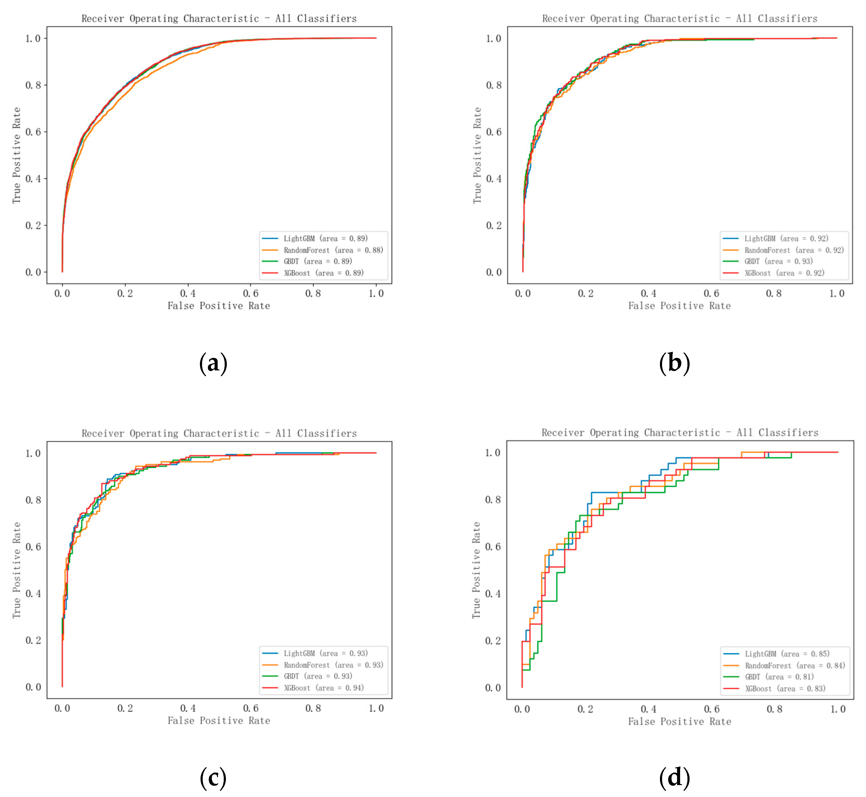
The model’s prediction results are shown in Figure 2. As can be seen in Figure 2a, under condition A (dry road conditions), the AUC is 0.89, which is consistent Wang et al. [18], who found that speed differentials signicantly impact similar to other machine learning models. The ROC curve indicates that the classifier performs quite well, although there is still room for improvement. The model shows good performance in distinguishing between different categories (accident severity). Dry road conditions provide better traction, which likely explains the relatively lower AUC score compared to other conditions.

In Figure 2b, under condition B (wet or water road surfaces), the AUC is 0.92, which is higher, slightly inferior to GBDT. This suggests that the model performs better in distinguishing accident severity under wet or waterlogged conditions. These road conditions generally lead to a higher accident rate, as vehicles may skid or lose traction, making it easier for the model to distinguish between different levels of accident severity.

Figure 2c shows that, under condition C (snow/slush/ice road conditions), the AUC is 0.93, indicating that the model can very accurately differentiate between levels of accident severity on icy or snowy roads, albeit slightly inferior to XGBoost. The increased difficulty in controlling vehicles on such surfaces leads to more severe accidents, which might explain the model’s strong performance in these extreme conditions.

In Figure 2d, under condition D (sand, mud, dirt, oil, or gravel road conditions), the AUC is 0.85, indicating that the model’s classification performance is poorer compared to other road conditions, outperformed by all of the other machine learning models. This may be due to the fact that vehicles exhibit various unstable behaviors on these complex surfaces, leading to more complex accident severity patterns, making it harder for the model to accurately predict and differentiate between accident types.

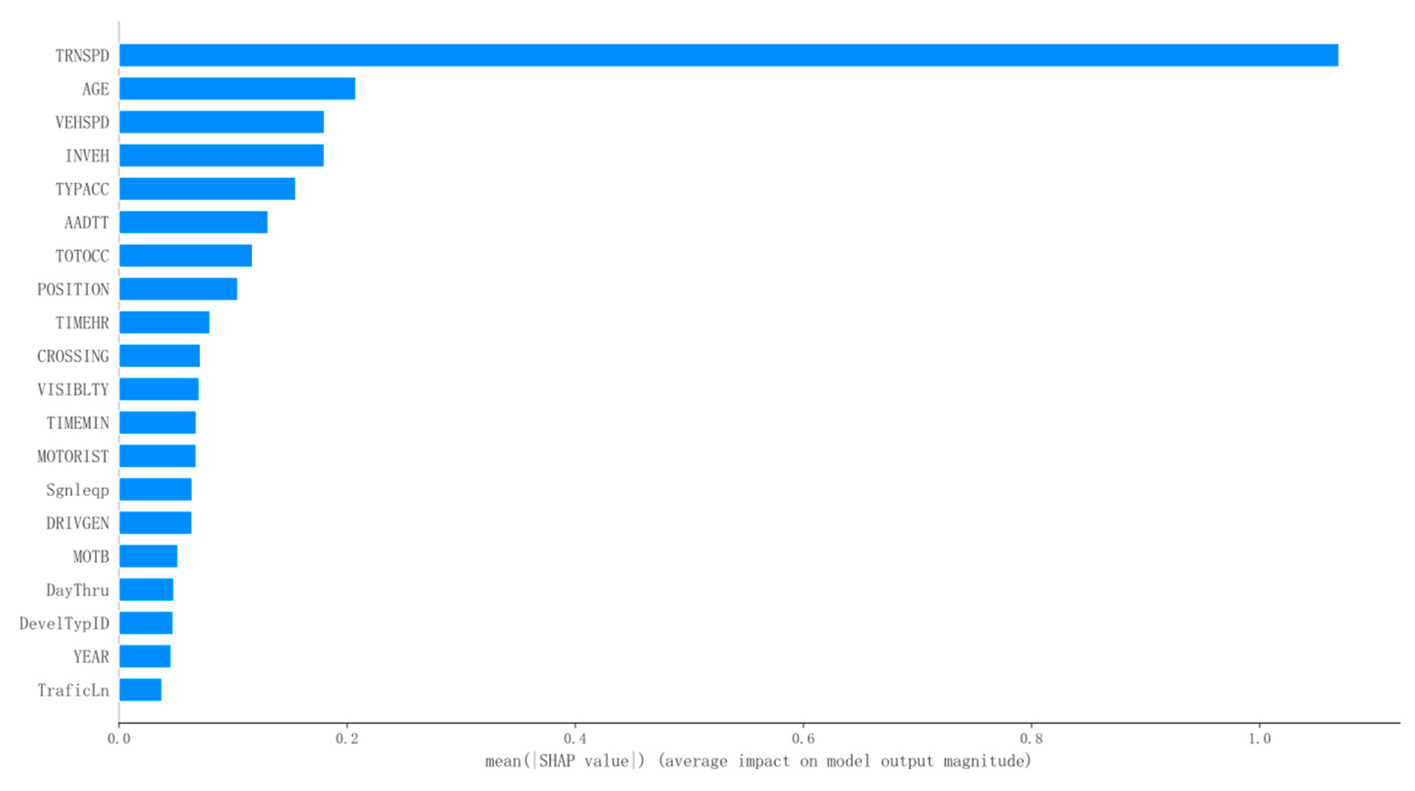
5.2. Importance of Risk Factors Not Grouped

First, the processed dataset was utilized to predict the severity of highway_rail grade crossing accidents, identifying the impact of various features across all road conditions. This served as a foundation for comparing the effects under different road conditions in subsequent analyses. In this study, SHAP was employed to interpret the LightGBM model, providing insights into the differences in the ranking of factors influencing accident severity.

Using the feature importance rankings derived from the SHAP model, the contributions and interactions of key factors affecting the severity of highway_rail grade crossing accidents were analyzed. Li et al. [19] demonstrated that driver behaviors, such as gap acceptance, play a significant role in influencing accident severity. This study further supports the importance of behavioral factors in determining outcomes, especially in complex driving enviroments. as illustrated in Figure 3. The results reveal that the five most influential features are “TRNSPD” (train speed), “AGE” (driver age), “VEHSPD” (vehicle speed), “INVEH” (whether the driver was inside the vehicle), and “TYPACC” (type of accident). However, feature importance alone does not fully account for the multicollinearity between these features, nor does it uncover the underlying mechanisms through which these factors exert their influence.

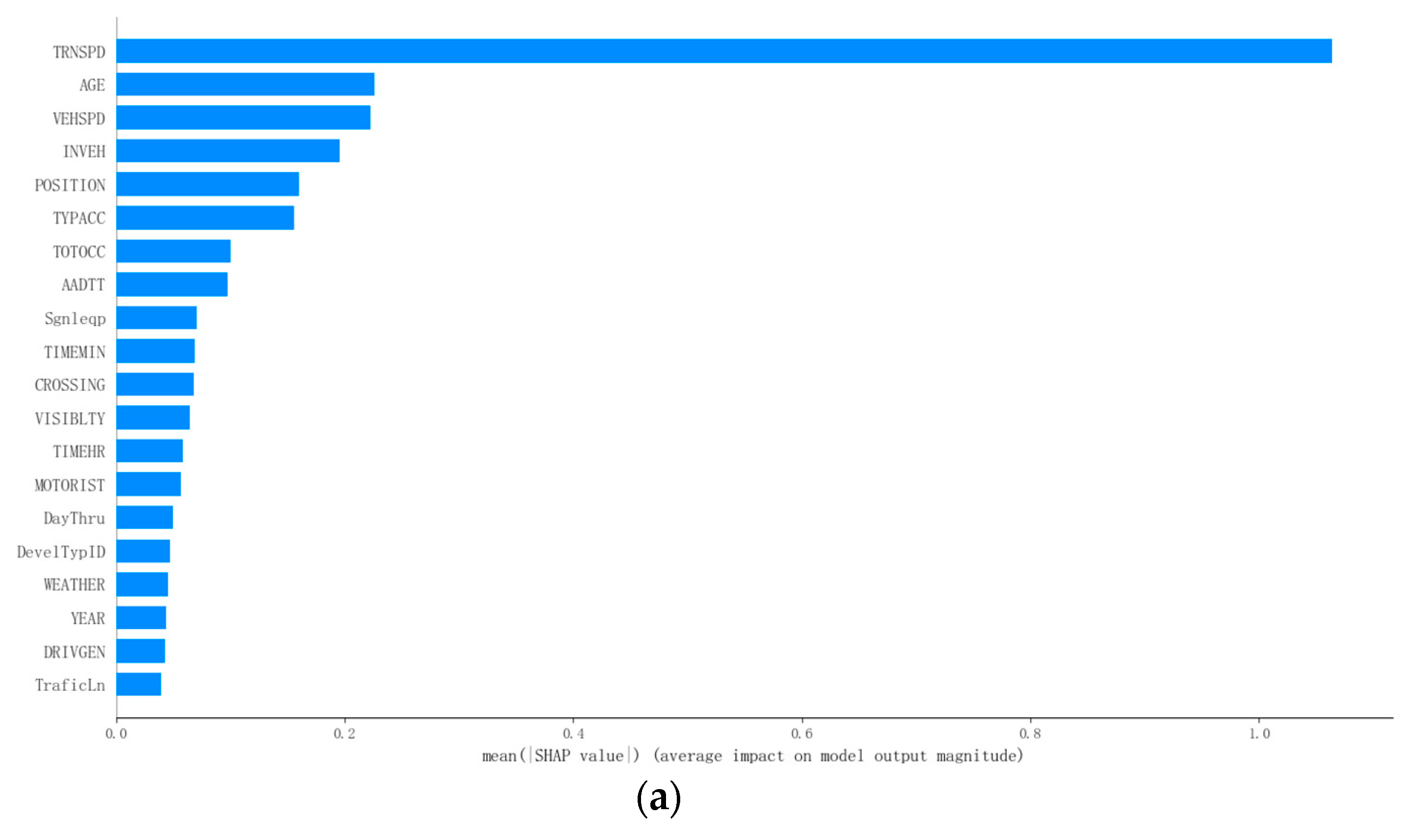
To assess the contribution of various features to the severity of highway_rail crossing accidents, a SHAP summary plot was generated, as shown in Figure 4. This study focuses on analyzing the top five factors influencing accident severity:

TRNSPD (train speed): As TRNSPD increases, the corresponding SHAP value also rises. This suggests that higher train speeds tend to result in more severe injuries for the driver, while lower train speeds lead to less severe accidents. The increased severity may be attributed to the reduced reaction time of the train driver at higher speeds, limiting the ability to take timely emergency actions. Additionally, higher train speeds increase braking distances, contributing to more serious injuries.

AGE (driver age): As the driver’s age increases, the SHAP value also increases, indicating that older drivers are more likely to suffer severe injuries. Younger drivers, on the other hand, tend to experience less severe accidents. This could be due to delayed brain responses in older drivers when confronted with sudden danger, preventing them from avoiding the hazard. In contrast, younger drivers generally react more quickly, allowing them to take emergency actions in time, thus reducing the severity of their injuries.

VEHSPD (vehicle speed): As VEHSPD increases, the SHAP value also rises, signifying that higher vehicle speeds are associated with more severe injuries. Lower vehicle speeds tend to result in less severe accidents. This may be due to the fact that higher vehicle speeds reduce the driver’s ability to make accurate judgments quickly, which can lead to more serious accidents, similar to the effect of high train speeds.

INVEH (driver inside the vehicle): It can be observed that when the driver is not inside the vehicle, the severity of injuries is lower compared to when the driver is inside. This is likely because the driver may take timely action to leave the vehicle upon recognizing imminent danger, reducing the extent of injury in a collision between the vehicle and the train.

TYPACC (type of accident): When “TYPACC” equals 1 (train collides with motor vehicle), it has a stronger positive impact on accident severity compared to when “TYPACC” equals 0 (motor vehicle collides with train). This is likely due to the greater kinetic energy of the train, which exerts a stronger force on the vehicle, leading to more severe accidents in train-to-vehicle collisions.

5.3. Importance of Risk Factors Grouped

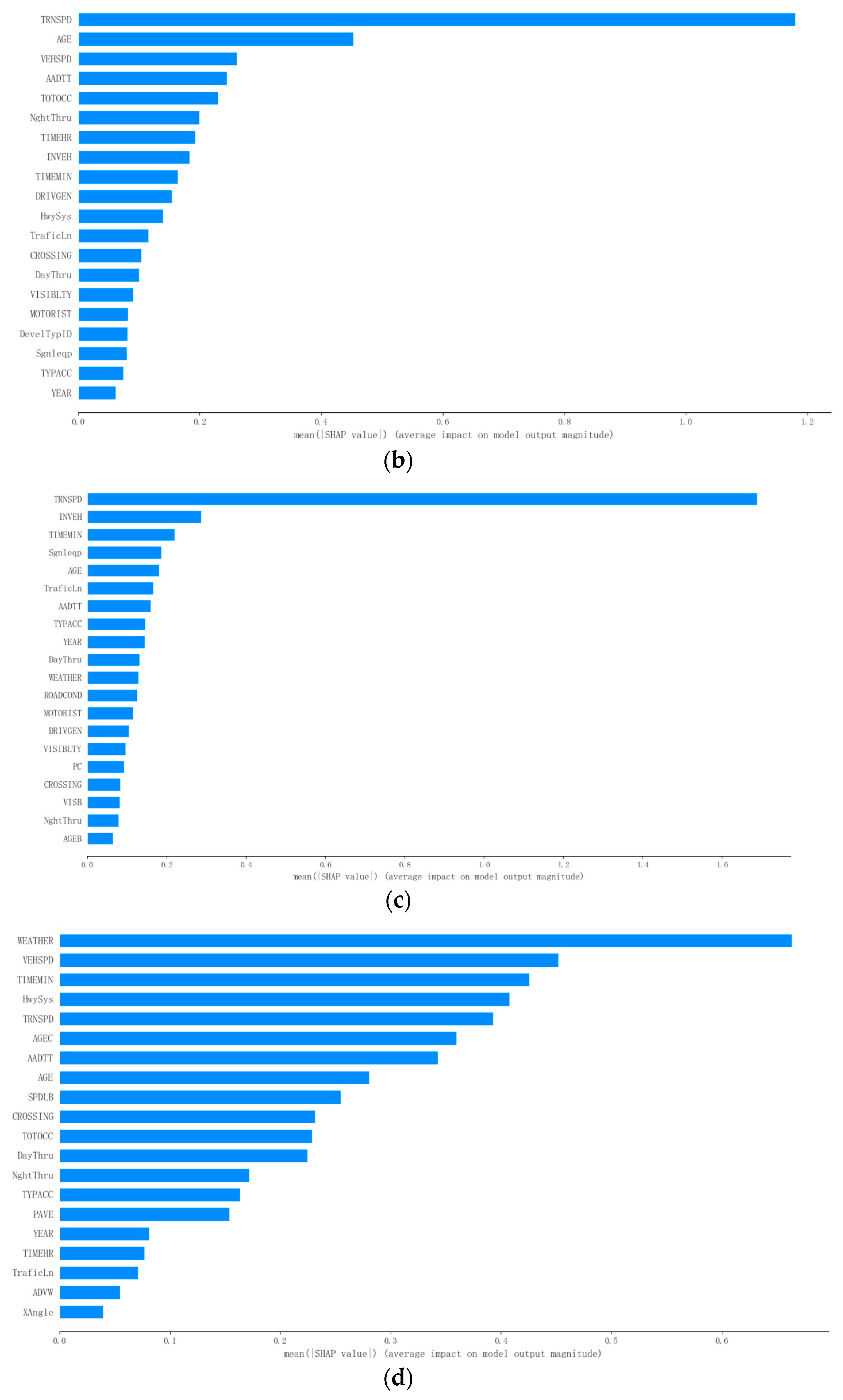
To evaluate the impact of different features on the severity of highway_rail grade crossing accidents under various road surface conditions, feature importance charts were created for the four road conditions, as shown in Figure 5.

Road Condition A (dry) (Figure 5a): The five most influential features affecting accident severity are “TRNSPD” (train speed), “AGE” (driver age), “VEHSPD” (vehicle speed), “INVEH” (whether the driver was in the vehicle), and “POSITION” (vehicle position).

Road Condition B (wet or with water) (Figure 5b): The top five influential features are “TRNSPD” (train speed), “AGE” (driver age), “VEHSPD” (vehicle speed), “AADTT” (average annual daily traffic), and “TOTOCC” (total occupants in the vehicle).

Road Condition C (snow, slush, or ice) (Figure 5c): The most influential features are “TRNSPD” (train speed), “INVEH” (whether the driver was in the vehicle), “TIMEMIN” (time in minutes), “Sgnleqp” (signal equipment), and “AGE” (driver age).

Road Condition D (sand, mud, dirt, oil, or gravel) (Figure 5d): The top five features are “WEATHER” (weather conditions), “VEHSPD” (vehicle speed), “TIMEMIN” (time in minutes), “HwySys” (highway rescue system), and “TRNSPD” (train speed).

To investigate the contributions of various factors to the severity of driver injuries in accidents at highway_rail grade crossings, SHAP force plots were generated for accident datasets under four road conditions, as shown in Figure 6. The results provide the following insights:

Pavement A (dry) (Figure 6a): Factors such as DRIVGEN = 1 (female drivers), INVEH = 1 (driver inside the vehicle), TYPACC = 1 (train colliding with a motor vehicle), and VEHSPD = 0 (vehicle speed) increase the severity of driver injuries. In contrast, TRNSPD = 14 (train speed) reduces the severity of injuries.

Pavement B (wet or with water) (Figure 6b): Under this condition, VISIBILITY = 1 (nighttime) and AADT = 2338 (average annual daily traffic) contribute to increased injury severity. However, factors such as TRNSPD = 40 (train speed), VEHSPD = 10 (vehicle speed), TOTOCC = 1 (single occupant), and INVEH = 0 (driver outside the vehicle) mitigate the severity of injuries.

Pavement C (snow, slush, or ice) (Figure 6c): Here, INVEH = 1 (driver inside the vehicle) increases the severity of driver injuries, while TRNSPD = 11 (train speed) has a mitigating effect.

Pavement D (sand, mud, dirt, oil, or gravel) (Figure 6d): Factors such as TRNSPD = 48 (train speed) and WEATHER = 1 (adverse weather conditions) contribute to increased injury severity. On the other hand, factors such as AGE = 20 (driver age), AADT = 20 (average annual daily traffic), and VEHSPD = 5 (vehicle speed) reduce the severity of injuries.

These findings highlight the influence of various contextual factors on the severity of driver injuries under different road conditions, providing valuable insights for targeted safety interventions.

The SHAP summary plots for each road condition, as shown in Figure 6, provide insights into the factors influencing the severity of highway–rail crossing accidents:

Pavement A (dry) (Figure 7a): The importance of the “POSITION” feature significantly increases, suggesting that when the vehicle is positioned as “moving over crossing”, “trapped on crossing by traffic”, or “blocked on crossing by gates”, accident severity tends to be higher. This is likely because, when a train is approaching, the vehicle being in these positions may prevent the driver from moving off the crossing in time, leading to more severe accidents. Additionally, it can be observed that as TRNSPD, AGE, and VEHSPD increase, the SHAP values also increase. This indicates that higher values of TRNSPD, AGE, and VEHSPD are associated with more severe injuries for the driver, while lower values of these factors are less likely to result in severe accidents. This may be due to higher speeds and older age reducing the driver’s reaction time and increasing braking distances when facing sudden events, thus amplifying the severity of the accident.

Pavement B (wet/standing water) (Figure 7b): The importance of “AADTT” (annual average daily traffic) and “TOTOCC” (total occupants) increases. This suggests that when the traffic volume is low and there are fewer vehicle occupants, drivers may feel safer and engage in more aggressive driving behaviors, disregarding the wet road conditions. Similarly, Wang et al. [20] observed that low traffic volumes often lead to increased risk-taking behavior, which correlates with higher accident severity. Combined with high train speeds, this reduces reaction times for both the driver and the train, potentially leading to severe accidents. Conversely, when the traffic volume is higher and there are more vehicle occupants, drivers are likely to be more cautious, leading to lower accident severity due to reduced vehicle and train speeds. Additionally, similar to Road Condition A, as TRNSPD, AGE, and VEHSPD increase, the SHAP values also increase. This indicates that higher values of TRNSPD, AGE, and VEHSPD contribute to more severe injuries for the driver, while lower values of these factors are less likely to result in severe accidents.

Pavement C (snow/ice) (Figure 7c): The importance of the “Sgnleqp” (signal equipment) feature increases, indicating that the presence of train signals reduces accident severity compared to crossings without signals. This may be because signals alert drivers, encouraging them to slow down or stop at the crossing, particularly on icy or snow-covered roads, thereby reducing the likelihood or severity of accidents. Additionally, it can be observed that higher TRNSPD tends to result in more severe injuries for the driver. Furthermore, when the driver is inside the vehicle, the severity of the accident increases. This may be due to the fact that drivers inside the vehicle are less likely to take timely self-rescue actions in the event of danger, which can lead to more severe outcomes.

Pavement D (sand, mud, oil, etc.) (Figure 7d): “WEATHER” emerges as the most influential factor, with clear or cloudy weather being linked to lower accident severity compared to rain, snow, or fog. This is likely because, despite the poor road surface, visibility is generally better in clear weather, allowing drivers more time to react and adjust their speed or route. In contrast, adverse weather conditions further degrade the road’s friction, increasing the risk of skidding or losing control. Li et al. [21] analyzed mandatory lane-changing behaviors under adverse road conditions and found that such behaviors significantly contribute to accident severity on unstable surfaces. Additionally, “HwySys” (highway rescue system) appears among the top five features for the first time. The presence of a rescue system can reduce response times and provide timely assistance, reducing the severity of the accident. In the absence of a rescue system, injured individuals may not receive prompt help, leading to more severe outcomes.

5.4. Influence of Risk Factors

To further understand the mechanisms by which various features influence the severity of highway_rail grade crossing accidents, SHAP dependency plots were generated for important features. These plots not only capture the main effects of individual factors but also reveal the interactions between two factors and how they influence accident severity, as illustrated in the figures.

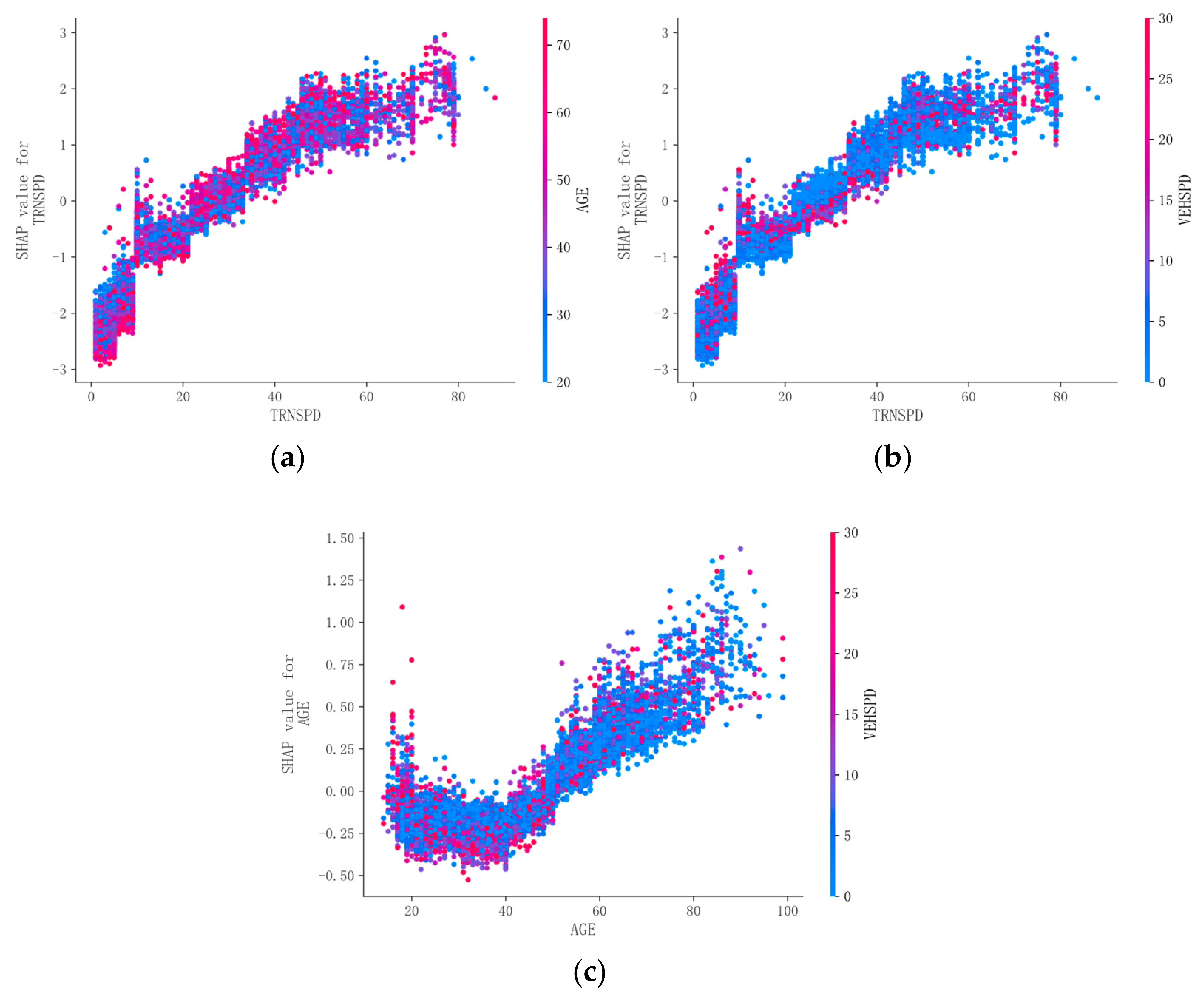
Under pavement A, as shown in Figure 8a,b, the impact of “TRNSPD” (train speed) on accident severity is significant, consistent with the findings of Pan Lu et al. A linear relationship can be observed between “TRNSPD” and accident severity. As TRNSPD increases, the SHAP value rises, indicating higher accident severity. However, once TRNSPD reaches 80, the SHAP value plateaus, suggesting that further increases in train speed do not significantly escalate accident severity. Additionally, “AGE” (driver age) and “VEHSPD” (vehicle speed) also significantly influence accident severity. Younger drivers and lower vehicle speeds are associated with more severe accidents. This could be because, on dry roads, vehicles have better traction, allowing drivers to maintain control at higher speeds. However, at very high speeds, the impact force increases dramatically, leading to more severe accidents. Younger drivers may also engage in more aggressive driving behaviors, contributing to greater accident severity.

As shown in Figure 8c, unlike other studies where the age threshold was set differently, this study diverges by setting the age boundary at 65 years. When “AGE” is less than 40, SHAP values show a decreasing trend with increasing age, indicating lower accident severity. However, when AGE exceeds 40, the relationship becomes linear, with the SHAP values increasing as AGE rises, suggesting higher accident severity. “VEHSPD” follows a similar pattern to AGE. This could be because younger drivers tend to react more quickly and handle sudden threats better at lower speeds, thus reducing accident severity. In contrast, older drivers traveling at higher speeds may experience longer braking distances, slower reaction times, and an increased likelihood of severe accidents due to these factors.

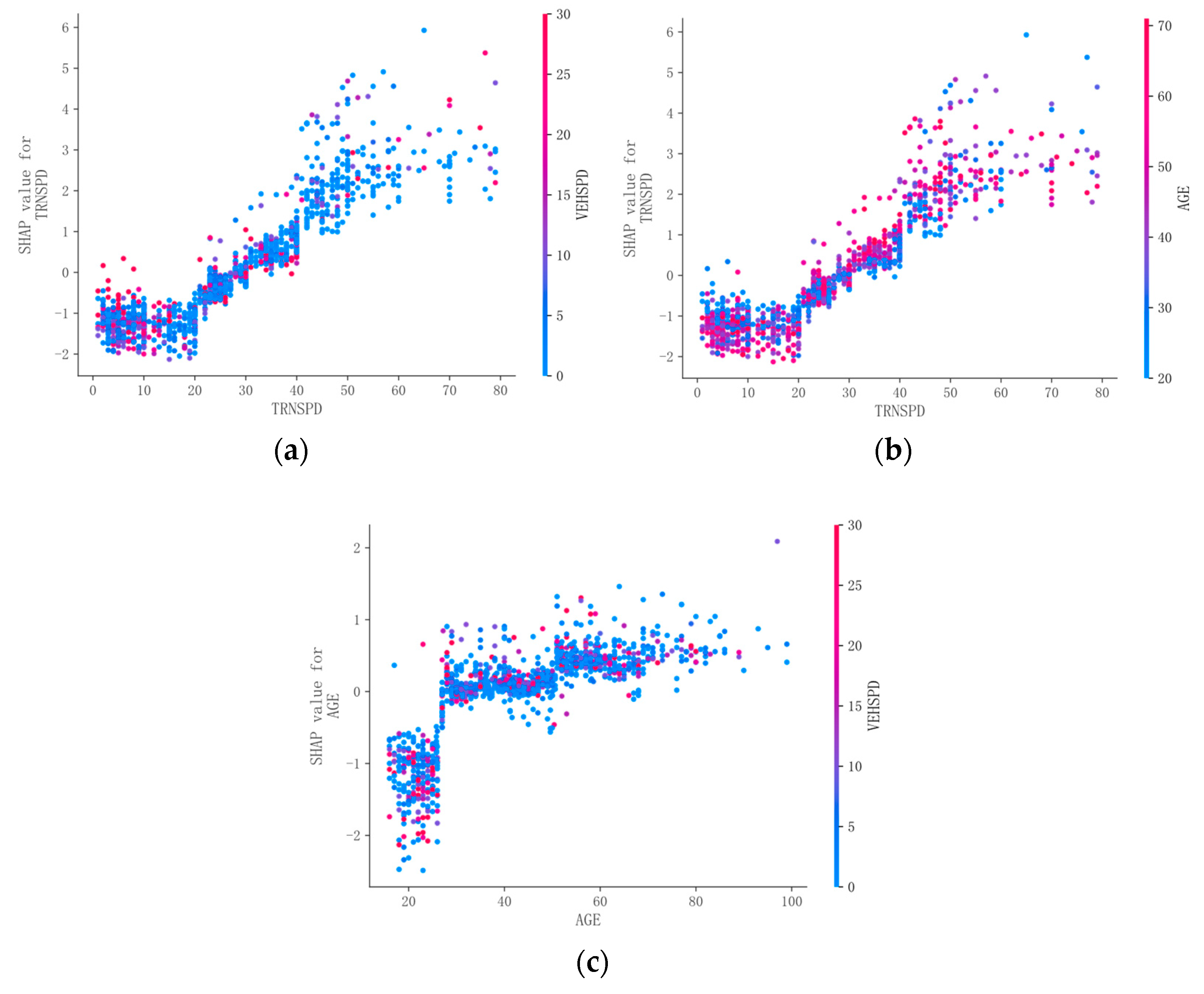
Under pavement B, as shown in Figure 9a,b, the impact of train speed on accident severity remains positively correlated within a certain range, similar to dry road conditions. However, the distribution of SHAP values exhibits greater volatility, particularly when the train speed is below 40. In this speed range, there is an almost linear relationship: the higher the train speed, the greater the accident severity. When the train speed exceeds 40, the distribution of SHAP values begins to flatten, indicating that further increases in speed do not lead to higher SHAP values.

Additionally, AGE and VEHSPD significantly affect accident severity. Older drivers and higher VEHSPD are more likely to be involved in serious accidents, possibly due to the slippery road conditions. Train speeds between 20 and 40 represent a critical range. Although the train speed is not high, factors such as slippery surfaces and increased braking distances reduce the driver’s control over the vehicle. Furthermore, older drivers may react more slowly, and higher speeds increase braking distances and reaction times, significantly impacting accident severity.

When train speed exceeds 40, the variability in SHAP values increases significantly, particularly in the 40–60 speed range, where the SHAP values fluctuate greatly. At this point, the impact of train speed on accident severity becomes nonlinear, possibly due to higher uncertainty at high speeds on wet surfaces, influenced by additional variables.

As shown in Figure 9c, when AGE is below 30, SHAP values exhibit greater volatility, especially around age 20, where the SHAP values are significantly higher than for other age groups. VEHSPD also has a substantial effect on accident severity, with higher speeds leading to more severe accidents. This may be due to younger drivers’ aggressive driving behaviors, their tendency to overlook road conditions due to insufficient driving experience, and their inability to respond effectively to sudden situations. In contrast, older drivers, who have more driving experience, can maintain better control of their vehicles even at higher speeds, thus reducing the severity of accidents.

Under pavement C, as shown in Figure 10, when the train speed (TRNSPD) is below 40, the SHAP values are relatively low, indicating a lower severity of accidents, regardless of whether the driver is inside the vehicle. However, when the train speed exceeds 40, particularly in the 40–70 range, the severity of accidents increases significantly when the driver is inside the vehicle. This increase in severity is likely due to the substantial difference in mass between trains and motor vehicles, which leaves the driver unable to react effectively in the event of a collision, resulting in more severe accidents.

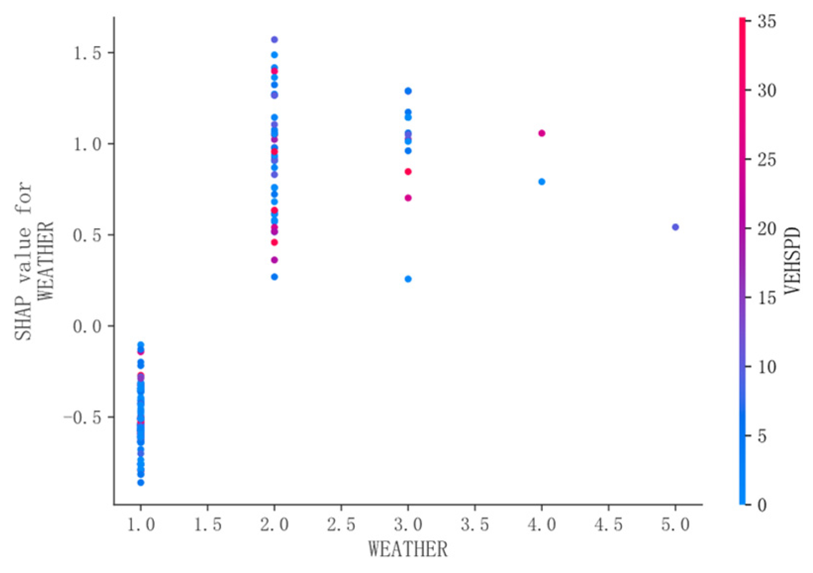
Under pavement D, as shown in Figure 11, the SHAP values are lower when the weather is clear, indicating lower accident severity. In contrast, under other weather conditions, the SHAP values are higher, suggesting a greater likelihood of severe accidents. This may be because, on sunny days, drivers benefit from better visibility and are more able to observe road conditions. When there is snow or ice, drivers tend to drive more cautiously, which reduces accident severity. However, in poor weather conditions, visibility decreases, making it difficult for drivers to accurately assess road conditions, potentially leading to more severe accidents.

When VEHSPD is below 20, SHAP values are low, indicating lower accident severity, regardless of when the accident occurs. However, when VEHSPD exceeds 20, the SHAP values increase, making severe accidents more likely. This may be due to the shorter braking distance of vehicles at lower speeds, which gives drivers sufficient reaction time, thus resulting in lower accident severity.

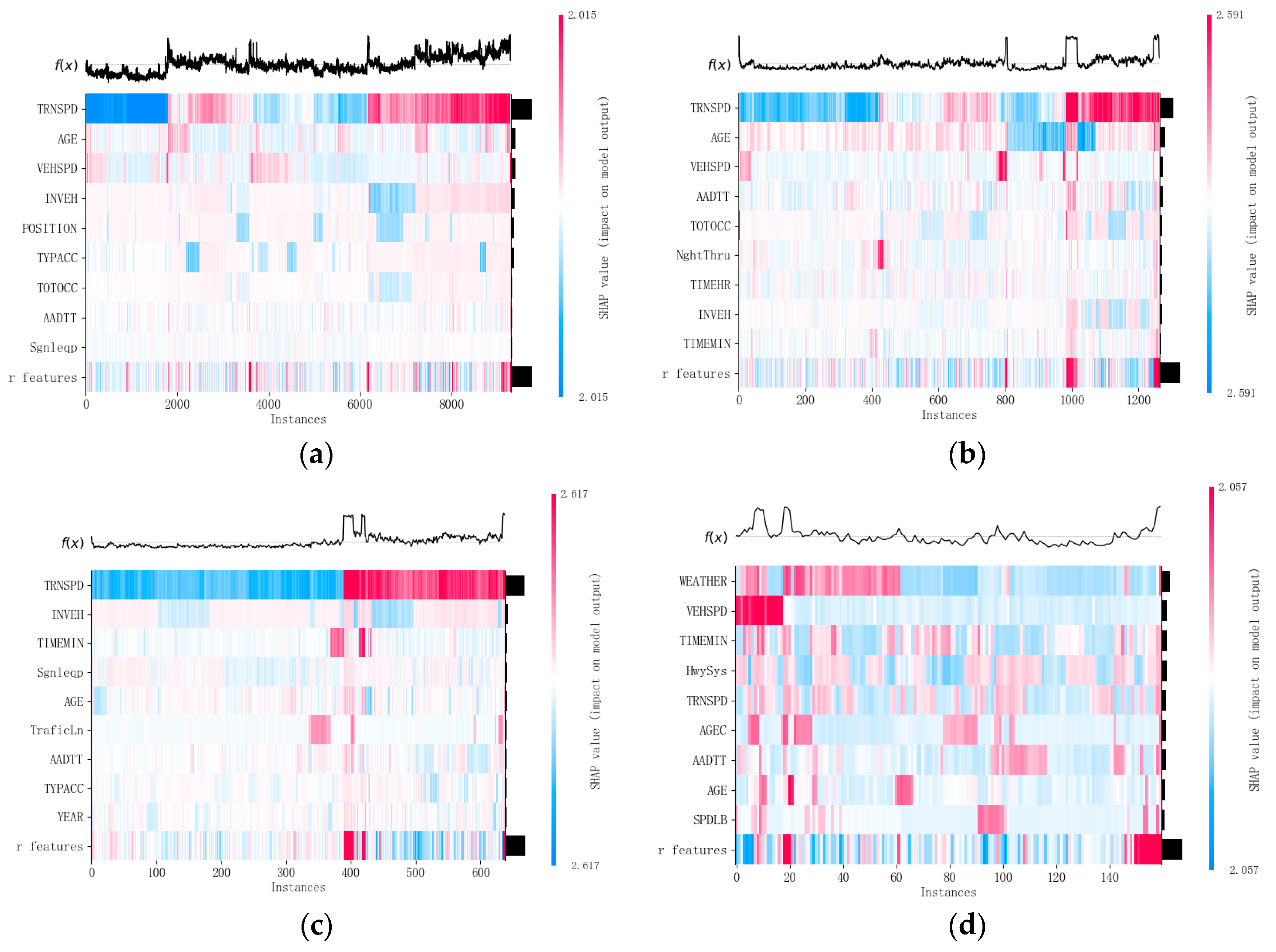
As shown in Figure 12a, under pavement A, f(x) is generally stable, although some peaks and valleys are still observed. The peaks correspond to higher predicted accident severity, while the valleys indicate lower predicted severity. Considering the SHAP values, in regions with higher f(x), the SHAP value for TRNSPD is shown in red, indicating that train speed has a significant positive contribution to predicting accident severity. Similarly, the SHAP values for AGE and VEHSPD also exhibit significant red areas in the high-accident-severity predictions, suggesting that higher speeds and older drivers increase accident severity.

In Figure 12b, under pavement B, f(x) shows larger fluctuations, with certain areas indicating a significant increase in predicted accident severity. TRNSPD continues to provide a strong positive contribution when predicting higher accident severity. Additionally, the SHAP values for AGE, AADT, and VEHSPD demonstrate a noticeable positive effect on predicting high accident severity, especially when AADT is high. Increased traffic volume on slippery roads significantly increases accident severity.

Figure 12c illustrates that, under pavement C, f(x) shows some prominent peaks, indicating that the model predicts higher accident severity in certain areas. In regions of predicted high accident severity, the SHAP values for TRNSPD and INVEH are positive, indicating a positive impact on accident severity. Furthermore, the influence of Sgnleqp becomes more significant, suggesting that the interaction between train speed and signaling equipment plays a major role in predicting high accident severity.

Figure 12d shows that, under pavement D, f(x) displays prominent peaks in certain areas. In regions of predicted high accident severity, the SHAP values for WEATHER and VEHSPD are positive, indicating that adverse weather conditions (rain, snow, fog) and higher VEHSPD have a positive impact on the prediction of accident severity.

6. Conclusions

This study utilizes interpretable machine learning to analyze the factors affecting the severity of driver injuries under different road surface conditions at highway–rail grade crossings. The dataset includes highway–rail grade crossing collision incidents that occurred in the United States from 2012 to 2021. After data cleaning, 14,198 cases were used for analysis. The LightGBM algorithm was employed to build models for four datasets, achieving high accuracy in predicting highway–rail grade crossing collision incidents. The SHAP method further enhanced the interpretability of the LightGBM algorithm by identifying important influencing factors and analyzing their impact and interactions in highway–rail grade crossing collisions.

The research results show the following:

• Under the condition of pavement A, the factors that have a greater impact on the severity of driver injury are TRNSPD, AGE, and VEHSPD. This study found that as TRNSPD (train speed), AGE, and VEHSPD (vehicle speed) increase, the severity of driver injuries also increases. Higher values of TRNSPD, AGE, and VEHSPD are often associated with more severe accidents, while lower values of these factors are less likely to result in high injury severity.
• Under the condition of pavement B, similar to the condition of pavement A, the factors that have a greater impact on the severity of driver injury are TRNSPD, AGE, and VEHSPD. Similar to pavement A, as the sample values of these three influencing factors increase, drivers are more likely to experience higher levels of injury severity.
• Under the condition of pavement C, the factors that have a greater impact on the severity of driver injury are TRNSPD and INVEH. It was also found that the driver being in the vehicle is more likely to lead to the occurrence of serious accidents.
• Under the condition of pavement D, unlike the previous three pavement conditions, the influence degree of TRNSPD is not that significant. Instead, weather conditions become the most prominent influencing factor. Drivers are more likely to be severely injured under severe weather conditions. Meanwhile, the influence of VEHSPD is also relatively significant.

The results of the analysis of influencing factors under different road surface conditions at highway–rail grade crossings provide valuable references and recommendations for the Federal Railroad Administration to implement targeted highway–rail grade crossing management strategies to prevent such incidents. The results indicate that the main factors affecting highway–rail grade crossing collisions are VEHSPD, TRN-SPD, AGE, AADT, and WEATHER. Specifically, under sand/mud/dirt/oil/gravel road surface conditions, WEATHER has the greatest impact compared to other road surface conditions, where its impact is relatively smaller.

This research, compared with other related studies, is mainly different in that it takes into account the influence of different pavement conditions on the severity of driver injuries in highway–rail grade crossing accidents, which may be an important factor overlooked by others. Moreover, in terms of methodology, the SHAP model interpreter was utilized to better analyze the degree of influence of different factors and their interactive effects. Meanwhile, this research also has similarities with other related studies. For example, train speed, vehicle speed, age, etc., are all factors with significant influence, which verifies the rationality of this research. It was also found that weather conditions have the greatest impact under pavement condition D, which echoes the research of other scholars on the influence of weather conditions on the severity of driver injuries in highway–rail grade crossing accidents. Perhaps further research could be conducted on the relationship between these two in the future.

There are several areas for improvement in this study. Factors such as VISIBILITY, DRIVGEN, and LIGHT at highway–rail grade crossings may also influence accident severity. Additionally, human factors, such as the driver’s level of education, vision, and personal driving habits, play an important role in accidents. Due to limited data, it was not possible to explore these factors in depth. Future research will aim to address these aspects. The main approaches and ideas are as follows:

• Enrich data sources: In addition to the existing accident data, more relevant data could be collected, such as the specific geographical information of the crossings, the temporal distribution of traffic flow, and the detailed weather data of different time periods, so as to analyze the factors affecting the safety of highway–rail grade crossings more comprehensively.
• Increase data dimensions: Consider collecting data on drivers’ health conditions, driving training records, and vehicle maintenance records, as well as the environmental data around the crossings, such as the nearby industrial pollution situation, noise level, etc. These factors may indirectly affect the driver’s state and the probability of accident occurrence.
• Conduct in-depth analysis of existing factors: For the identified main influencing factors, such as VEHSPD, TRNSPD, AGE, AADT, WEATHER, etc., further investigation of their complex interrelationships and the variation laws in different scenarios would be beneficial. Through more in-depth data analysis and professional knowledge, the potential influencing mechanisms could be explored.
• Incorporate new factors: The factors that have not been fully explored, such as VISIBILITY, DRIVGEN, LIGHT, etc., could be incorporated into the research scope, analyzing their synergistic effects with the existing factors and their independent impacts on accident severity, thereby constructing a more comprehensive and accurate model.
• Optimize the model algorithm: Research could attempt to use other advanced machine learning algorithms or improve the existing LightGBM algorithm to improve the prediction accuracy and generalization ability of the model. Meanwhile, the performance of different algorithms could be compared to select the model structure that is most suitable for this problem.

References

1. Wang, C.; Chen, F.; Zhang, Y.; Cheng, J. Analysis of injury severity in rear-end crashes on an expressway involving different types of vehicles using random-parameters logit models with heterogeneity in means and variances. Transp. Lett. 2023, 15, 742–753. [Google Scholar] [CrossRef]
2. Lu, P.; Zheng, Z.; Ren, Y.; Zhou, X.; Keramati, A.; Tolliver, D.; Huang, Y. A Gradient Boosting Crash Prediction Approach for Highway-Rail Grade Crossing Crash Analysis. J. Adv. Transp. 2020, 2020, 6751728. [Google Scholar] [CrossRef]
3. Zheng, Z.; Lu, P.; Pan, D. Predicting Highway-Rail Grade Crossing Collision Risk by Neural Network Systems. J. Transp. Eng. Part A Syst. 2019, 145, 04019033. [Google Scholar] [CrossRef]
4. Pasha, J.; Dulebenets, M.A.; Abioye, O.F.; Kavoosi, M.; Moses, R.; Sobanjo, J.; Ozguven, E.E. A Comprehensive Assessment of the Existing Accident and Hazard Prediction Models for the Highway-Rail Grade Crossings in the State of Florida. Sustainability 2020, 12, 4291. [Google Scholar] [CrossRef]
5. Rana, P.; Sattari, F.; Lefsrud, L.; Hendry, M. Machine Learning Approach to Enhance Highway Railroad Grade Crossing Safety by Analyzing Crash Data and Identifying Hotspot Crash Locations. Transp. Res. Record 2024, 2678, 1055–1071. [Google Scholar] [CrossRef]
6. Gao, L.; Lu, P.; Ren, Y. A Deep Learning Approach for Imbalanced Crash Data in Predicting Highway-Rail Grade Crossings Accidents. Reliab. Eng. Syst. Saf. 2021, 216, 108019. [Google Scholar] [CrossRef]
7. Keramati, A.; Lu, P.; Iranitalab, A.; Pan, D.; Huang, Y. A Crash Severity Analysis at Highway-Rail Grade Crossings: The Random Survival Forest Method. Accid. Anal. Prev. 2020, 144, 105683. [Google Scholar] [CrossRef] [PubMed]
8. Hao, W.; Daniel, J. Motor Vehicle Driver Injury Severity Study under Various Traffic Control at Highway-Rail Grade Crossings in the United States. J. Saf. Res. 2014, 51, 41–48. [Google Scholar] [CrossRef] [PubMed]
9. Hao, W.; Daniel, J. Driver Injury Severity Related to Inclement Weather at Highway-Rail Grade Crossings in the United States. Traffic Inj. Prev. 2016, 17, 31–38. [Google Scholar] [CrossRef] [PubMed]
10. Hao, W.; Kamga, C. Difference in Rural and Urban Driver-Injury Severities in Highway-Rail Grade Crossing Accidents. Int. J. Inj. Control Saf. Promot. 2017, 24, 174–182. [Google Scholar] [CrossRef] [PubMed]
11. Wang, R.; Chu, H.; Liu, Q.; Chen, B.; Zhang, X.; Fan, X.; Wu, J.; Xu, K.; Jiang, F.; Chen, L. Application of Machine Learning Techniques to Improve Multi-Radar Mosaic Precipitation Estimates in Shanghai. Atmosphere 2023, 14, 1364. [Google Scholar] [CrossRef]
12. Kavoosi, M.; Dulebenets, M.A.; Pasha, J.; Abioye, O.F.; Moses, R.; Sobanjo, J.; Ozguven, E.E. Development of Algorithms for Effective Resource Allocation among Highway-Rail Grade Crossings: A Case Study for the State of Florida. Energies 2020, 13, 1419. [Google Scholar] [CrossRef]
13. Hao, W.; Kamga, C. The Effects of Lighting on Driver’s Injury Severity at Highway-Rail Grade Crossings. J. Adv. Transp. 2016, 50, 446–458. [Google Scholar] [CrossRef]
14. Hao, W.; Kamga, C.; Daniel, J. The Effect of Age and Gender on Motor Vehicle Driver Injury Severity at Highway-Rail Grade Crossings in the United States. J. Saf. Res. 2015, 55, 105–113. [Google Scholar] [CrossRef] [PubMed]
15. Hajihosseinlou, M.; Maghsoudi, A.; Ghezelbash, R. A Novel Scheme for Mapping of MVT-Type Pb-Zn Prospectivity: LightGBM, a Highly Efficient Gradient Boosting Decision Tree Machine Learning Algorithm. Nat. Resour. Res. 2023, 32, 2417–2438. [Google Scholar] [CrossRef]
16. Ke, G.; Meng, Q.; Finley, T.; Wang, T.; Chen, W.; Ma, W.; Ye, Q.; Liu, T.-Y. LightGBM: A Highly Efficient Gradient Boosting Decision Tree. In Proceedings of the Advances in Neural Information Processing Systems 30 (NIPS 2017), Long Beach, CA, USA, 4–9 December 2017; Guyon, I., Luxburg, U.V., Bengio, S., Wallach, H., Fergus, R., Vishwanathan, S., Garnett, R., Eds.; Neural Information Processing Systems (nips): La Jolla, CA, USA, 2017; Volume 30. [Google Scholar]
17. Lundberg, S.M.; Lee, S.-I. A Unified Approach to Interpreting Model Predictions. In Proceedings of the Advances in Neural Information Processing Systems 30 (NIPS 2017), Long Beach, CA, USA, 4–9 December 2017; Guyon, I., Luxburg, U.V., Bengio, S., Wallach, H., Fergus, R., Vishwanathan, S., Garnett, R., Eds.; Neural Information Processing Systems (nips): La Jolla, CA, USA, 2017; Volume 30. [Google Scholar]
18. Wang, W.; Yang, Y.; Yang, X.; Gayah, V.V.; Wang, Y.; Tang, J.; Yuan, Z. A negative binomial Lindley approach considering spatiotemporal effects for modeling traffic crash frequency with excess zeros. Accid. Anal. Prev. 2024, 207, 107741. [Google Scholar] [CrossRef] [PubMed]
19. Li, G.; Zhao, L.; Wu, L.; Jiang, C.; Tang, W. Investigating gap acceptance behavior based on correlated random parameter survival model with heterogeneity in means. Transp. Lett. 2024, 1–16. [Google Scholar] [CrossRef]
20. Wang, C.; Mohamed, A.-A.; Lei, H. Effects of speed difference on injury severity of freeway rear-end crashes: Insights from correlated joint random parameters bivariate probit models and temporal instabil-ity. Anal. Methods Accid. Res. 2024, 42, 100320. [Google Scholar] [CrossRef]
21. Li, G.; Zhao, L.; Tang, W.; Wu, L.; Ren, J. Modeling and analysis of mandatory lane-changing behavior considering heterogeneity in means and variances. Phys. A Stat. Mech. Its Appl. 2023, 622, 128825. [Google Scholar] [CrossRef]
Figure 1. Schematic diagram of the LightGBM method.
Symmetry 17 00147 g001
Figure 2. ROC metrics: (a) ROC curve of LightGBM under pavement A; (b) ROC curve of LightGBM under pavement B; (c) ROC curve of LightGBM under pavement C; (d) ROC curve of LightGBM under pavement D.
Symmetry 17 00147 g002
Figure 3. Feature variable importance based on the SHAP model.
Symmetry 17 00147 g003
Figure 4. SHAP summary plots.
Symmetry 17 00147 g004
Figure 5. Feature variable importance based on SHAP model: (a) Analysis of factors related to pavement A. (b) Analysis of factors related to pavement B. (c) Analysis of factors related to pavement C. (d) Analysis of factors related to pavement D.
Symmetry 17 00147 g005aSymmetry 17 00147 g005b
Figure 6. SHAP force plots: (a) The SHAP force plot for pavement A. (b) The SHAP force plot for pavement B. (c) The SHAP force plot for pavement C. (d) The SHAP force plot for pavement D.
Symmetry 17 00147 g006
Figure 7. SHAP summary plots: (a) The SHAP summary plots for pavement A. (b) The SHAP summary plots for pavement B. (c) The SHAP summary plots for pavement C. (d) The SHAP summary plots for pavement D.
Symmetry 17 00147 g007aSymmetry 17 00147 g007b
Figure 8. SHAP interaction effects plots: (a) SHAP interaction effects plot of TRNSPD and AGE under pavement A; (b) SHAP interaction effects plot of TRNSPD and VEHSPD under pavement A; (c) SHAP interaction effects plot of AGE and VEHSPD under pavement A.
Symmetry 17 00147 g008
Figure 9. SHAP interaction effects plots: (a) SHAP interaction effects plot of TRNSPD and VEHSPD under pavement B; (b) SHAP interaction effects plot of TRNSPD and AGE under pavement B; (c) SHAP interaction effects plot of AGE and TRNSPD under pavement B.
Symmetry 17 00147 g009
Figure 10. SHAP interaction effects plot of TRNSPD and INVEH under pavement C.
Symmetry 17 00147 g010
Figure 11. SHAP interaction effects plot of WEATHER and VEHSPD under pavement D.
Symmetry 17 00147 g011
Figure 12. Feature importance plots: (a) The feature importance plot for pavement A. (b) The feature importance plot for pavement B. (c) The feature importance plot for pavement C. (d) The feature importance plot for pavement D.
Symmetry 17 00147 g012