High-Performance Carrier Phase Recovery for Local Local Oscillator Continuous-Variable Quantum Key Distribution

Abstract

Continuous-variable quantum key distribution (CV-QKD) has been increasingly studied, which offers the advantage of compatibility with modern coherent optical communication systems. In contrast to CV-QKD with a transmitting local oscillator, the local local oscillator CV-QKD avoids the security vulnerabilities of a local oscillator by generating a local oscillator at the receiver. In practice, the frequency offset of the two lasers introduces extra phase noise, which is generally suppressed by various carrier phase recovery algorithms. However, the accuracy of carrier phase recovery can be influenced by the power of the pilot tone, particularly as the transmission distance increases. To further improve accuracy, we propose a method based on the unscented particle filter algorithm, to increase the accuracy of phase estimation, effectively restore the quantum signal and reduce excess noise. In our work, we demonstrated a local local oscillator CV-QKD experiment with a finite-size block of $1\times {10}^8$ under a transmission distance of 50 km. Through our method, we achieved a secret key rate of 525 kbps, which represents a 28% improvement. These results confirm that our proposed method not only improves the accuracy of carrier phase recovery, but also provides a new approach for future research on algorithms for long-distance CV-QKD. Furthermore, our study improves the phase compensation performance, enabling the orthogonal components of the quantum signal to exhibit enhanced symmetry in phase space.

1. Introduction

Quantum key distribution (QKD) is a technology based on the principles of quantum mechanics that ensures secure key distribution between two parties [1,2,3]. Quantum key distribution can be achieved through two approaches: discrete-variable QKD and continuous-variable QKD (CV-QKD). Among them, the CV-QKD protocol has garnered significant attention due to its low implementation cost and superior compatibility with modern optical communication systems. CV-QKDs have been extensively studied, encompassing in-depth theoretical analysis [4,5,6,7,8,9,10,11,12,13] and extensive experimental validation [14,15,16,17,18,19,20,21,22,23,24]. According to the modulation methods of the coherent state, two practical CV-QKD schemes have been proposed: one is based on Gaussian modulation coherent state (GMCS) and the other is based on the discrete modulation coherent state (DMCS) [5,6,8]. The GMCS CV-QKD protocol, which was proposed earlier, already has a relatively mature composable security proof [7]. Due to its ability to carry more information, enabling a higher secret key rate in the same distance, compared to the DMCS protocol, the Gaussian modulation has become the most widely used modulation scheme in CV-QKD.

CV-QKD experimental systems can be classified into two types based on the location of the local oscillator (LO): the transmitting local oscillator (TLO) scheme and the local local oscillator (LLO) scheme. In the TLO scheme, the LO is generated at the transmitter and transmitted along with the signal, but the TLO scheme faced challenges such as LO power attenuation over long distances and security vulnerabilities [25,26], prompting extensive research. Since the proposal of the LLO scheme in 2015 [27,28], the LLO scheme, which generates the LO at the receiver, has gained significant attention, enhancing security and simplifying system implementation, compared to the TLO scheme. The LLO scheme allows the application of advanced digital signal processing (DSP) techniques [29,30,31] from modern coherent optical communication systems to address issues such as phase drift and device imperfections. Although this introduces the complexity of security analysis [32], a new digital signal processing analysis method has recently been proposed to address this issue, providing a solid foundation for the design and security evaluation of DSP systems [10].

In LLO CV-QKD, researchers have explored the use of high-power pilot tone [15], transmitted alongside the quantum signal, to assist in carrier phase recovery. These methods typically multiplex the pilot tone and quantum signal using techniques such as time, polarization, or frequency division [33,34,35]. In summary, regardless of the multiplexing method used, the effectiveness of all these techniques heavily relies on the accuracy of phase estimation for the pilot tone [36], highlighting the necessity for further advancements in carrier recovery methods. Given the critical role of accurate phase estimation for pilot tone, current research has increasingly focused on Bayesian filtering algorithms. A long-distance CV-QKD experiment based on a locally generated LO was successfully conducted over a 100 km fiber channel by using the Kalman filter (KF) [22]. Additionally, KF was employed to estimate the misalignment of the quantum signal’s polarization state, compensating for dynamic changes caused by random birefringence effects, significantly improving the accuracy of polarization error estimation [30]. In another study, the application of the unscented Kalman filter (UKF) over a 20 km fiber-optic link demonstrated that UKF could maintain very low excess noise even under low pilot power conditions [37]. Meanwhile, a particle filter (PF) was also applied in a four-user quantum downstream access network, demonstrating that, over a transmission distance of 10 km, the four users achieved secret key rates of 546 kbps, 535 kbps, 522.5 kbps, and 512.5 kbps, respectively, while successfully maintaining low levels of excess noise [21]. But they all have certain limitations. KF struggles in nonlinear and high-noise environments, the computational complexity of PF grows with particle numbers, and UKF, while addressing nonlinearity, remains computationally intensive and sensitive to parameter tuning. Therefore, investigating more effective phase recovery algorithms is crucial to further enhancing the accuracy of phase estimation in practical LLO CV-QKD.

In this paper, we proposed a high-performance carrier phase recovery method based on the unscented particle filter (UPF) algorithm to improve the accuracy of phase estimation in LLO CV-QKD. The UPF algorithm enhances phase estimation accuracy by combining the UKF and PF algorithms. By utilizing the unscented transformation (UT) [38], the UPF improves the prediction of the prior probability distribution, which aids the particle filter in addressing high-dimensional, nonlinear and non-Gaussian problems. This method also optimized particle weight distribution, mitigated weight degradation, and reduced the need for resampling. Based on this algorithm, we demonstrated a LLO CV-QKD experiment with a transmission distance of 50 km, where the UPF algorithm was employed to estimate the pilot tone’s phase. In contrast, we successfully reduced excess noise to 0.0048 SNU, achieving a secret key rate of 525 kbps, which represents a 28% improvement. These results confirm that the method we proposed improves the accuracy of carrier phase recovery and provides a solution for more effective and precise carrier phase recovery algorithms in future research on long-distance CV-QKD.

The rest of the paper is organized as follows: In Section 2, we model the phase prediction in LLO CV-QKD, providing a detailed description of the UPF algorithm’s process and principles. In Section 3, we present a point-to-point 50km LLO CV-QKD experiment, including the digital signal processing. In Section 4, we demonstrate the performance of the UPF algorithm from the perspective of security parameters. Finally, we draw conclusions in Section 5.

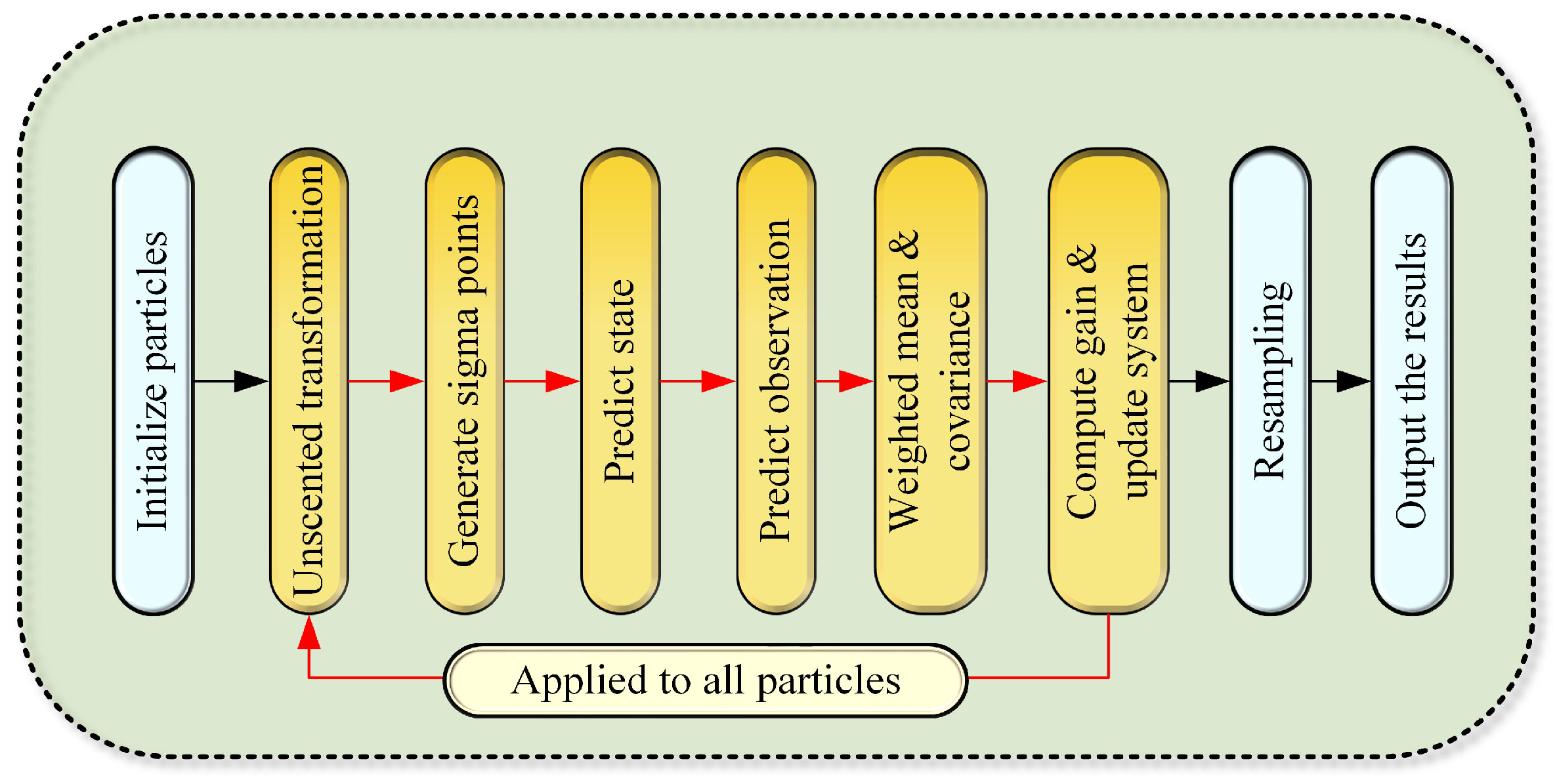
2. A Phase Prediction Model Based on Unscented Particle Filter

In the UPF algorithm, the state-space model is commonly used to represent real-world systems. The state-space model is a time-domain framework for describing the characteristics of dynamic systems, where time acts as an implicit independent variable. It consists of two key equations, the mathematical representation of a state-space model is typically expressed as follows:

$$x_t=f(x_{t-1},w_t),$$

(1)

where $x_t$ denotes the system state at time t, $w_t$ is the process noise, accounting for uncertainties in the state dynamics, the input to the state model is typically the phase of the pilot tone, $f(·)$ is the state function.

$$z_t=g(x_t,v_t),$$

(2)

where $z_t$ denotes the observation or measurement at time t, $v_t$ represent the observation noise, capturing measurement uncertainties, $g(·)$ is the observed function. Since the recursive from of Bayesian filter is based on the posterior probability density of nonlinear systems, it does not require the assumption that $w_t$ and $v_t$ are zero-mean Gaussian white noise. This framework provides a robust foundation for modeling and analyzing dynamic systems.

In the practical LLO CV-QKD, we need to model the state equations and observation equations to conduct better analysis. We record the cosine or sine value of the pilot tone’s phase observed at time $1\to t$ as $z_{1:t}$, where the state variable $x_t$ represents the value of the pilot tone’s phase, and the corresponding expression is as follows:

$$x_{1:t}=[{\theta }_{fas{t}_0},{\theta }_{fas{t}_1},\cdots ,{\theta }_{fas{t}_{t-1}}],$$

(3)

$$z_{1:t}=[cos\left({\theta }_{fas{t}_1}\right),cos\left({\theta }_{fas{t}_2}\right),\cdots ,cos\left({\theta }_{fas{t}_t}\right)],$$

(4)

where ${\theta }_{fas{t}_t}$ represents the pilot tone’s phase at the t time, which is used to compensate for rapid frequency drift, and the $cos\left({\theta }_{fas{t}_t}\right)$ as the observed value, corresponding to the cosine and sine components of the pilot tone’s phase in practical LLO CV-QKD. When considering process noise, the model update is as follows:

$$x_t={\theta }_{fas{t}_{t-1}}+w_t,\hspace{1em}{z}_t=cos\left({\theta }_{fas{t}_t}\right)+v_t.$$

(5)

After introducing the phase prediction model of LLO CV-QKD, we now focus on the key steps of the UPF:

Prediction: In the case, assuming the probability density function at time $t-1$ is known, as $p\left(x_{t-1}\right|z_{1:t-1})$, the prior probability density function of the state at time t can be predicted based on the dynamic Equation (2). The prior probability density function at time k can be expressed as follows:

$$\begin{array}{c}\hfill \begin{array}{cc}\hfill p\left(x_t\right|z_{1:t-1})& =\int p(x_t,x_{t-1}|z_{1:t-1})p\left(x_{t-1}\right|z_{1:t-1})\mathrm{d}{x}_{t-1}\hfill \\ \hfill & =\int p\left(x_t\right|x_{t-1})p\left(x_{t-1}\right|z_{1:t-1})\mathrm{d}{x}_{t-1},\hfill \end{array}\end{array}$$

(6)

where $z_{1:t-1}$ represents the observed quantities, and $x_t$ is the unknown system variable, which follows a first-order Markov process, corresponding to the pilot tone’s phase to be predicted, this implicitly assumes $p\left(x_t\right|x_{t-1})=p\left(x_t\right|x_{t-1},z_{1:t-1})$. $p\left(x_t\right|x_{t-1})$ is the state transition probability density function of the system.

Update: Once new observations become available, the update step adjusts the predicted state by incorporation the observed date. At the current time t, the observation $z_t$ is obtained using the system measurement model. Base on this observation, the prior probability density function $p\left(x_t\right|z_{1:t-1})$ is updated to derive the posterior probability density function $p\left(x_t\right|z_{1:t})$ at time t. Based on Bayes’theorem, the calculation of the posterior probability can be expressed as

$$p\left(x_t\right|z_{1:t})={\displaystyle \frac{p\left(z_t\right|x_t)p\left(x_t\right|z_{1:t-1})}{p\left(z_t\right|z_{1:t-1})}},$$

(7)

where $p\left(z_t\right|z_{1:t-1})$ can be obtained using the following formula:

$$p\left(x_t\right|z_{1:t-1})=\int p\left(z_t\right|x_t)p\left(x_t\right|z_{1:t-1})\mathrm{d}{x}_t.$$

(8)

The particle filter approximates the posterior state distribution using weighted random particles [39]. These particles are drawn from an importance density function, adjusted based on state observation, and used to estimate the posterior distribution. The state estimate is obtained by the weighted sum of these particles.

Typically, according to the known prior probability $p\left(x_t\right)$, the initialization generates N particles, and the initial set of particles $x_t^{\left(i\right)}$, and then the new particles are generated based on the state transition function as $x_{t+1}^{\left(i\right)}\sim p\left(x_t\right|x_{t-1}^{\left(i\right)})$, the weight of each particle $\omega {\left(i\right)}_{i=1}^N$ is ${\displaystyle \frac{1}{N}}$. Next, the weights are updated based on the importance density function, denoting the importance density function as $q\left(x_{0:t}\right|z_{1:t})$, the weight update formula is given by

$$\begin{array}{c}\hfill \begin{array}{cc}\hfill & {\omega }_t^{\left(i\right)}\infty {\displaystyle \frac{p\left(x_{0:t}^{\left(i\right)}\right|z_{1:t})}{q\left(x_{0:t}^{\left(i\right)}\right|z_{1:t})}},\hfill \\ \hfill & ={\displaystyle \frac{p\left(z_t\right|x_t^{\left(i\right)})p\left(x_t^{\left(i\right)}\right|x_{t-1}^{\left(i\right)})p\left(x_{0:t-1}^{\left(i\right)}\right|z_{1:t-1})}{q\left(x_t^{\left(i\right)}\right|x_{0:t-1}^{\left(i\right)},z_{1:t})q\left(x_{0:t-1}^{\left(i\right)}\right|z_{1:t-1})}}\hfill \\ \hfill & ={\omega }_{t-1}^{\left(i\right)}{\displaystyle \frac{p\left(z_t\right|x_t^{\left(i\right)})p\left(x_t^{\left(i\right)}\right|x_{t-1}^{\left(i\right)})}{q\left(x_t^{\left(i\right)}\right|x_{0:t-1}^{\left(i\right)},z_{1:t})}},\hfill \end{array}\end{array}$$

(9)

where $q\left(x_{0:t}^{\left(i\right)}\right|z_{1:t})$ represents the importance density function, which can be decomposed as $q\left(x_t^{\left(i\right)}\right|x_{0:t-1}^{\left(i\right)},z_{1:t})q\left(x_{0:t-1}^{\left(i\right)}\right|z_{1:t-1})$, and $p\left(x_{0:t}^{\left(i\right)}\right|z_{1:t})$ represents the posterior probability density function, expressed as $p\left(z_t\right|x_t^{\left(i\right)})p\left(x_t^{\left(i\right)}\right|x_{t-1}^{\left(i\right)})p\left(x_{0:t-1}^{\left(i\right)}\right|z_{1:t-1})$, then to normalize the weights, the formula is as follows:

$${\widehat{\omega }}_t^{\left(i\right)}={\displaystyle \frac{{\omega }_t^{\left(i\right)}}{{\sum }_{i=0}^N{\omega }_t^{\left(i\right)}}}.$$

(10)

Then, we apply the unscented transformation to each particle set, after resampling, the posterior probability estimate is obtained:

$${\widehat{x}}_t=\sum _{i=0}^N{\chi }_t^{\left(i\right)\sigma }{\widehat{\omega }}_t^{\left(i\right)},$$

(11)

where the ${\chi }_t^{\left(i\right)\sigma }$ denotes the set of sigma points generated by the particle set $x_t^{\left(i\right)}$. The UPF extends the standard particle filter by incorporating the unscented Kalman filter [40], which better approximates the state distribution in highly nonlinear systems. The flowchart of the UPF algorithm is shown in Figure 1, see further details in Appendix A.

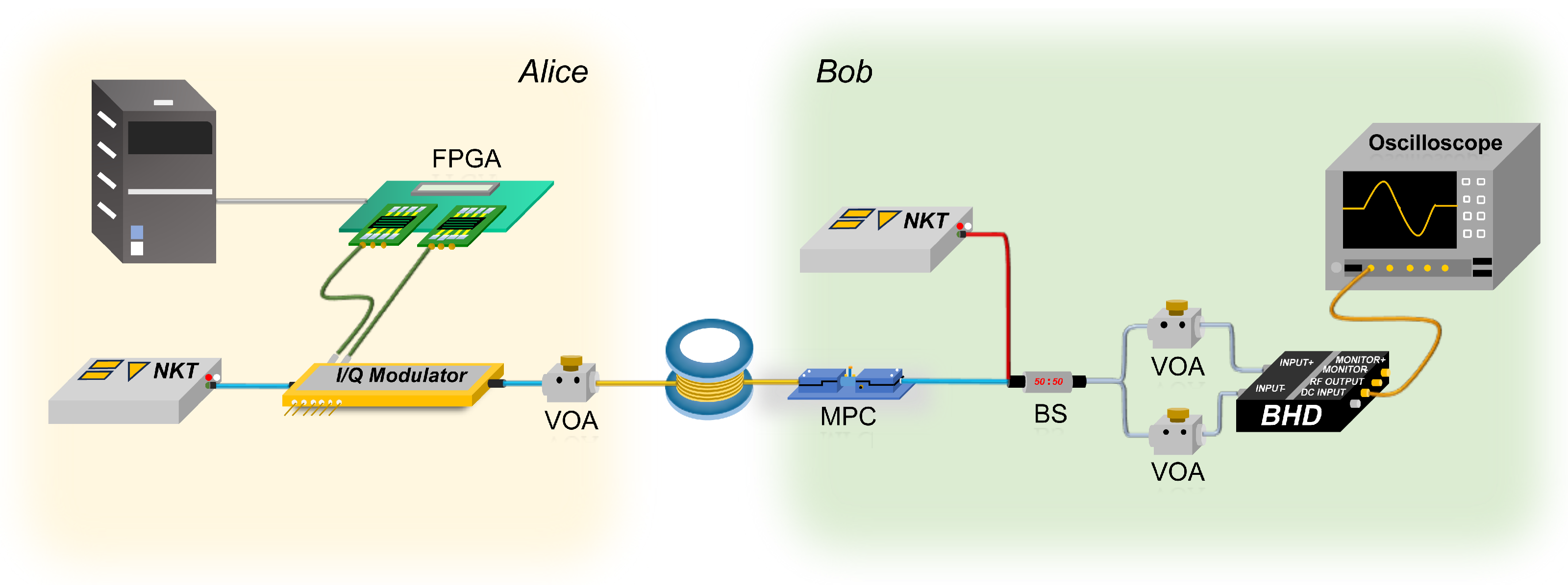
3. Local Local Oscillator CV-QKD Experimental Scheme

3.1. Experimental Setup

In our work, we successfully implemented a LLO CV-QKD experiment, the experimental setup is depicted in Figure 2. A continuous laser with a narrow linewidth is employed at Alice’s side to generate coherent light, which has a wavelength of 1550.12 nm. Then, the GMCS signals, operating at a repetition frequency of $100\mathrm{MHz}$, are generated as the continuous-wave light passes through an IQ modulator. The modulation process is driven by a self-developed 16bit DAC board integrated into the FPGA. It is worth noting that during this process, a bias controller was used to ensure the IQ modulator operates stably at an optimal operating point over an extended period. Additionally, we employed an implementation of pilot-sequential LLO structure, we controlled the IQ modulator using electrical signals output by the FPGA to achieve the alternate transmission of the pilot tone and quantum signal. In this process, the quantum signal follows a Rayleigh distribution for its amplitude and a uniform distribution for its phase. Subsequently, the signal is directed through a variable optical attenuator (VOA) positioned after the IQ modulator, this step ensures the quantum signal is attenuated to achieve the optimal modulation variance $V_A$, ensuring the GMCS signals are attenuated to the quantum signal level, thereby exhibiting quantum characteristics. Finally, in our experiment, a quantum channel consists of standard optical fibers with a total length of $50\mathrm{km}$.

At Bob’s side, the signal is first directed into a manual polarization controller (MPC), which compensates for polarization loss during channel transmission, ensuring optimal polarization state alignment. Another laser generates the LO, with sufficient power to meet the limit of shot-noise-limited detection requirements of quantum signal, and its operating wavelength is also stabilized at 1550.12 nm. Subsequently, the signal and LO interfere stably within a beam splitter (BS) equipped with a fast-axis cut off. The outputs from the BS are individually connected to VOAs, which are finely adjusted to achieve optical path and intensity balance for the signals entering the detector. Notably, we employ a balanced homodyne detector (BHD) with a $1.6\mathrm{GHz}$ bandwidth for detection. Finally, the output electrical signals are collected using a real-time oscilloscope operating at $1\mathrm{GSa}/\mathrm{s}$ for data acquisition.

3.2. Digital Signal Processing Based on UPF Algorithm

After acquiring the data, the quantum signal cannot be directly obtained. To address this, signal processing is required based on the frequency difference between the two lasers. Before initiating the processing, we define several variables to facilitate a clear explanation of the procedure. The quantum signal and pilot tone before the BHD can be expressed as follows:

$$E_{sig}=A_{sig}cos(2\pi f_{A}t+{\varphi }_{sig}+{\phi }_{sig}+{\phi }_{channel,sig}),$$

(12)

$$E_{ref}=A_{ref}cos(2\pi f_{A}t+{\phi }_{ref}+{\phi }_{channel,ref}),$$

(13)

where $f_A$ denotes the center frequency of Alice’s laser, and ${\varphi }_{sig}$ refers to the Gaussian modulated phase. Additionally, $A_{sig}$ and $A_{ref}$ represent the amplitude values of the quantum signal and reference signal, respectively. ${\phi }_{sig}$ and ${\phi }_{ref}$ represent initial phase of the laser. ${\phi }_{channel,sig}$ and ${\phi }_{channel,ref}$ denote the phase difference between the quantum signal and pilot tone when they meet in the channel. Then the LO can be expressed as follows:

$$E_{LO}=A_{LO}cos(2\pi f_{B}t+{\phi }_{LO}),$$

(14)

where $A_{LO}$ represents the amplitude values of the LO, $f_B$ denotes the center frequency of Bob’s laser, and ${\phi }_{LO}$ represents initial phase. Therefore, we can obtain the expression for the photocurrent:

$$\begin{array}{c}\hfill \begin{array}{cc}\hfill I_{sig}& =R\eta \left(\right|E_{sig}+E_{LO}{|}^2-|E_{sig}-E_{LO}{|}^2)\hfill \\ \hfill & =2R\eta A_{sig}{A}_{LO}cos(2\pi \Delta f_{AB}t+{\varphi }_{sig}+\Delta {\phi }_{fast}+\Delta {\phi }_{slow}),\hfill \end{array}\end{array}$$

(15)

$$\begin{array}{c}\hfill \begin{array}{cc}\hfill I_{ref}& =R\eta \left(\right|E_{ref}+E_{LO}{|}^2-|E_{ref}-E_{LO}{|}^2)\hfill \\ \hfill & =2R\eta A_{ref}{A}_{LO}cos(2\pi \Delta f_{AB}t+\Delta {\phi }_{fast}),\hfill \end{array}\end{array}$$

(16)

where R and $\eta$ represent the responsiveness and detection efficiency of the BHD, the $\Delta f_{AB}$ is caused by the frequency difference between the two lasers. $\Delta {\phi }_{fast}$ is defined as the phase variation caused by rapid frequency drift, while the initial phase difference between the reference signal and the quantum signal is defined as $\Delta {\phi }_{slow}$.

Then, we first perform a frequency offset estimation on the collected electrical signals using Fourier transform to determine the value of $\Delta f_{AB}$, which is approximately $248\mathrm{MHz}$. After that, we utilize the frequency $\Delta f_{AB}$ to obtain the X and P orthogonal components by the exponential function $e^{-2\pi \Delta f_{AB}t}$, both the quantum and pilot tone. Additionally, a low-pass filter is applied with carefully chosen parameters. Finally, the process can be shown as follows:

$$\begin{array}{c}\hfill \begin{array}{cc}\hfill X_{sig}& =LPF\left(real\left(I_{sig}{e}^{-2\pi \Delta f_{AB}t}\right)\right)\hfill \\ \hfill & =R\eta A_{LO}{A}_{sig}cos({\varphi }_{sig}+\Delta {\phi }_{fast}+\Delta {\phi }_{slow}),\hfill \end{array}\end{array}$$

(17)

$$\begin{array}{c}\hfill \begin{array}{cc}\hfill P_{sig}& =LPF\left(imag\left(I_{sig}{e}^{-2\pi \Delta f_{AB}t}\right)\right)\hfill \\ \hfill & =-R\eta A_{LO}{A}_{sig}sin({\varphi }_{sig}+\Delta {\phi }_{fast}+\Delta {\phi }_{slow}),\hfill \end{array}\end{array}$$

(18)

$$\begin{array}{c}\hfill \begin{array}{cc}\hfill X_{ref}& =LPF\left(real\left(I_{ref}{e}^{-2\pi \Delta f_{AB}t}\right)\right)\hfill \\ \hfill & =R\eta A_{LO}{A}_{ref}cos(\Delta {\phi }_{fast}),\hfill \end{array}\end{array}$$

(19)

$$\begin{array}{c}\hfill \begin{array}{cc}\hfill P_{ref}& =LPF\left(imag\left(I_{ref}{e}^{-2\pi \Delta f_{AB}t}\right)\right)\hfill \\ \hfill & =-R\eta A_{LO}{A}_{ref}sin(\Delta {\phi }_{fast}),\hfill \end{array}\end{array}$$

(20)

where $LPF(·)$ denotes the low-pass filter function, and we used a third-order bandpass Butterworth filter with a band width of approximately 50 MHz. $real(·)$ represents the real part extraction of the orthogonal components, and $imag(·)$ represents the imaginary part extraction of the orthogonal components. After this, we can calculate the $\Delta {\phi }_{fast}$ using the pilot tone.

$${\theta }_{fast}=-ta{n}^{-1}(P_{ref}/X_{ref}).$$

(21)

Based on the Equation (21), the phase information carried by the pilot tone can be obtained, allowing us to compensate for the quantum signal. In theory, by using ${\theta }_{fast}$, the $\Delta {\phi }_{fast}$ component in the quantum signal can be compensated for. However, due to the influence of the additive noises, they do not match exactly. Consequently, direct compensation introduces errors, which in turn increase the excess noise. To address the issue of inaccurate estimation of the ${\theta }_{fast}$, we propose the UPF algorithm to improve the accuracy of the phase estimation, the specific UPF prediction model has be introduced in the Section 2. In this process, the ${\theta }_{fast}$ is taken as the state variable of the UPF, where the state function $f\left({\theta }_{fast}\right)$ is equal to the current value of the ${\theta }_{fast}$, and the $X_{ref}$ and $P_{ref}$ are used as the observations. The process is expressed as follows:

$${\widehat{\theta }}_{fast}=UPF\left({\theta }_{fast}\right|X_{ref},P_{ref}).$$

(22)

Afterwards, the calculated angle is used to perform the corresponding phase compensation as follows:

$$\begin{array}{c}\hfill \begin{array}{cc}\hfill X_{sig}^{\prime }& =X_{sig}cos({\widehat{\theta }}_{fast})-P_{sig}sin({\widehat{\theta }}_{fast})\hfill \\ \hfill & =R\eta A_{LO}{A}_{sig}cos({\varphi }_{sig}+\Delta {\phi }_{slow}),\hfill \end{array}\end{array}$$

(23)

$$\begin{array}{c}\hfill \begin{array}{cc}\hfill P_{sig}^{\prime }& =-X_{sig}sin({\widehat{\theta }}_{fast})-P_{sig}cos({\widehat{\theta }}_{fast})\hfill \\ \hfill & =-R\eta A_{LO}{A}_{sig}sin({\varphi }_{sig}+\Delta {\phi }_{slow}).\hfill \end{array}\end{array}$$

(24)

In the final stage of the DSP, a segmented compensation approach is used. For each segment of data, Alice shares a portion of the initial data with Bob, then Bob searches for compensation values within the range of $0\sim 2\pi$, and calculates the correlation between the compensated results and the shared data. The $\Delta {\phi }_{slow}$ is compensated through the selection of the ${\theta }_{slow}$ corresponding to the moment with the maximum correlation. Since the $\Delta {\phi }_{slow}$ is generally a constant with minimal fluctuation, an appropriate compensation segment length can ensure effective compensation. The received components $X_B$ and $P_B$ can be represented as follows:

$$\begin{array}{c}\hfill \begin{array}{cc}\hfill X_B& =X_{sig}^{\prime }cos\left({\theta }_{slow}\right)-P_{sig}^{\prime }sin\left({\theta }_{slow}\right)\hfill \\ \hfill & =R\eta A_{LO}{A}_{sig}cos\left({\varphi }_{sig}\right),\hfill \end{array}\end{array}$$

(25)

$$\begin{array}{c}\hfill \begin{array}{cc}\hfill P_B& =-X_{sig}^{\prime }sin\left({\theta }_{slow}\right)-P_B^{\prime }cos\left({\theta }_{slow}\right)\hfill \\ \hfill & =-R\eta A_{LO}{A}_{sig}sin\left({\varphi }_{sig}\right).\hfill \end{array}\end{array}$$

(26)

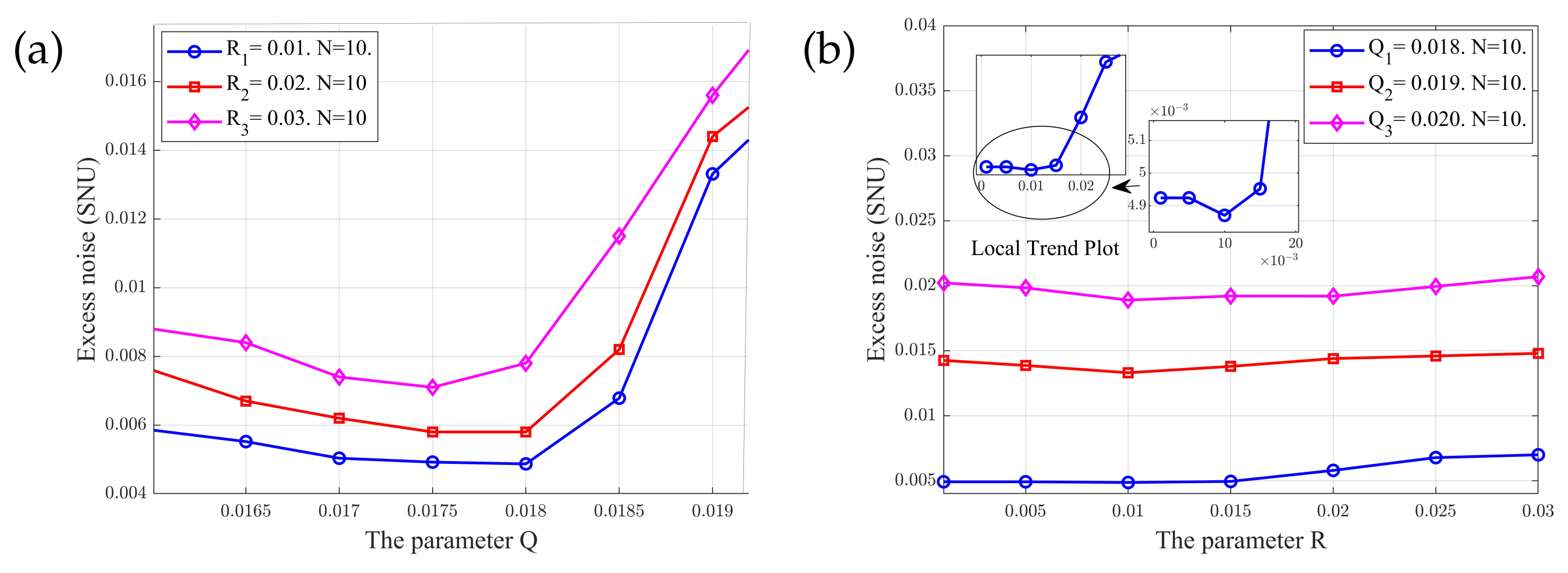
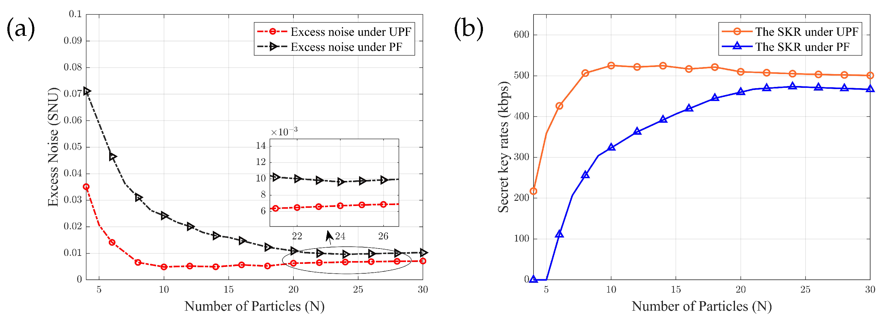
4. Experimental Results and Analysis

Upon establishing the experimental system and processing the data, we successfully acquired the processed Gaussian-modulated signals. Initially, we performed the calibration of certain parameters, normalizing them to SNU units, as these parameters are critical for subsequent parameter estimation. After completing the parameter estimation, we derived key system performance metrics, including excess noise, and the secret key rates for the practical implementation of this scheme. The calibrated parameters are summarized in

Table 1. The parameters calibrated for the experimental system.

Transmission Distance (km)	Modulation Variance (SNU)	Detection Efficiency	Electric Noise (SNU)	Reconciliation Efficiency
50	4.01	0.481	0.0271	0.95

.

Here, we consider the finite-size block effect, the secret key rates (SKR) can be expressed as follows:

$$K=f·{\displaystyle \frac{n}{N}}(\beta I_{AB}-{\chi }_{BE}-\Delta \left(n\right)),$$

(27)

where f indicates the repetition frequency of the quantum signal, N represents the total length of the raw data, and n specifies the data length allocated for key extraction. The reconciliation efficiency is denoted by $\beta$, while $I_{AB}$ quantifies the Shannon mutual information between Alice and Bob, and ${\chi }_{BE}$ is the Holevo bound, representing the maximum information available to Eve, the eavesdropper, about Bob’s key. $\Delta \left(n\right)$ is a parameter representing the impact of the finite-size block effect on the system security during the process of the privacy amplification. See the further details of the calculations in Appendix B.

Immediately after, we can provide the experimental excess noise and the corresponding secret key rates under different parameters of the UPF filter. We define $w_t$ as independent and identically distributed system noise with variance Q, and $v_t$ as independent and identically distributed measurement noise with Gaussian distribution and variance R. We compare the excess noise under different parameters Q and R, and finally determine the most optimal parameters. We investigated the variation of excess noise under different parameters Q and R, as shown in Figure 3, with the same particle number N = 10. Figure 3a illustrates the curve of excess noise in the system for varying values of parameter Q. In the figure, three solid lines in different colors correspond to different values of parameter R. The range of Q values was chosen between 0.016 and 0.02, as smaller values of Q lead to an excessively small particle net, causing resampling failure. As observed, for parameter Q values below 0.018, the excess noise decreases gradually, eventually reaching a minimum. However, for values of Q exceeding 0.018, the excess noise increases sharply. This is due to the fact that with a fixed number of particles, excessively large values of Q introduce significant errors, resulting in inaccurate estimates. Figure 3b presents the variation of excess noise with parameter R. The three solid lines in different colors represent the results for different reference values of parameter Q. It can be observed that as parameter R increases, the change in excess noise is minimal. However, a closer inspection of the blue inset reveals that excess noise still exhibits a minimum value when R is equal to 0.01. Beyond this threshold, when the value of R exceeds 0.01, the excess noise increases. Notably, when parameter $Q_1$ is set to 0.018, the overall excess noise is lower than the values for $Q_2$ and $Q_3$, which is consistent with the results shown in Figure 3a.

In addition, we also verified the relationship between the accuracy of the UPF and PF algorithms and the number of particles N, the results are shown in the Figure 4. Figure 4a illustrates the relationship between excess noise and particle number for the two algorithms. The red dashed line represents the variation in particle number and excess noise under the UPF algorithm. As shown in the figure, when the value of N is 10, the excess noise reaches around 0.005 SNU, and as N increases, the excess noise fluctuates within this range. The black dashed line indicates the change in particle number and excess noise under PF filtering. It is evident that when N reaches 20, the excess noise reaches around 0.01 SNU, with a slower convergence rate compared to the UPF algorithm. At the same time, Figure 4b illustrates the relationship between secret key rates and particle numbers. When the number of particles is the same, the UPF algorithm achieves a higher secret key rate. This demonstrates that the proposed UPF algorithm, utilizing fewer particles than PF, achieves lower excess noise and higher secret key rates, ensuring improved performance with reduced the number of particles.

Immediately following this, we describe the change in the secret key rates and excess noise in 10 h, and the results are shown in Figure 5. Lower marks represent excess noise, corresponding to the initial excess noise, the excess noise processed by PF with 20 particles, and the excess noise processed by UPF with 10 particles, from top to bottom. Meanwhile upper marks indicate the secret key rates, where are the initial secret key rates, the secret key rates after PF with 20 particles, and the secret key rates after UPF with 10 particles, from top to bottom. This also demonstrates the advantages of the proposed algorithm in terms of higher secret key rates and lower excess noise.

Subsequently, we examine the pilot tone’s phase results before and after filtering. As illustrated in Figure 6, the purple points denote the distribution of pilot tone’s phase variations within the range of $-\pi$ to $\pi$ before UPF filtering, whereas the red points indicate the refined distribution after UPF filtering. Evidently, before UPF filtering, the phase variation exhibits a larger fluctuation range compared to after UPF filtering. The UPF algorithm demonstrates its effectiveness in compensating for pilot tone’s phase variations and substantially mitigating noise. We calculated the residual phase noise before and after UPF filtering, the results show that the excess noise caused by residual phase noise was 0.0118 SNU before UPF filtering and reduced to 0.00377 SNU after UPF filtering. This advanced filtering approach enhances the precision of the $\Delta {\phi }_{fast}$ filtering process, leading to a marked reduction in excess noise.

Therefore, we performed parameter estimation on the data before and after compensation, yielding the results shown in Figure 7. The secret key rates and excess noise before and after UPF compensation are illustrated, where parameter estimation was conducted on ten sets of data over a period of time. In the figure, the blue line represents the secret key rates, and the orange line represents the excess noise. From Figure 7a, it can be observed that before UPF compensation, the mean excess noise averages ${\epsilon }_1$ around 0.0157 SNU, indicating that inaccurate phase estimation contributes to additional excess noise. In Figure 7b, it is clearly seen that after UPF compensation, the mean excess noise ${\epsilon }_2$ drops to around 0.005 SNU, demonstrating the precise compensation provided by UPF. In addition, it can be seen in the figure that the mean of the secret key rates $SK{R}_2$ after UPF filtering is significantly higher than $SK{R}_1$.

The experimental and simulated results of the secret key rates corresponding to different transmission distances are illustrated in Figure 8. The black line represents the PLOB bound [41] for the GMCS CV-QKD protocol. The red solid line shows the variation of the secret key rates with transmission distance after UPF filtering under the assumption of an infinite-size block. In contrast, the blue solid line represents the relationship between the secret key rates and transmission distance before UPF filtering under the same assumption. It is evident that the secret key rates after filtering are consistently higher than those before filtering. Furthermore, the red dashed line indicates the secret key rates as a function of transmission distance after UPF filtering with a finite-size block of $1\times {10}^8$, while the blue dashed line depicts the same relationship without UPF filtering. Notably, the blue diamond and red star markers represent the calculated secret key rates at a transmission distance of 50 km. At a repetition frequency of 100 MHz, only 50 MHz of the quantum signal is effectively utilized. Therefore, the secret key rates are calculated to be 409 kbps and 525 kbps before and after applying the UPF filtering, respectively. This demonstrates a significant improvement in the secret key rates, with an increase of approximately 28%, rising from 409 kbps to 525 kbps, after UPF filtering.

5. Conclusions

In this paper, we propose a high-performance carrier phase recovery method for LLO CV-QKD based on the UPF algorithm. The UPF algorithm improves particle filtering by incorporating the unscented transformation, enhancing the accuracy of phase estimation for pilot tone. To evaluate the performance of the UPF algorithm, we demonstrate a pilot-sequential structure LLO CV-QKD experiment with a transmission distance of 50 km. The experimental results show that, with the implementation of the UPF algorithm, the excess noise is reduced from 0.0157 SNU to 0.0048 SNU, and the secret key rates increase by approximately 28%, from 409 kbps to 525 kbps. Additionally, we validate that the UPF algorithm outperforms the traditional particle filter method by achieving lower excess noise with fewer particles, significantly reducing computational complexity. These results highlight the significant advantages of the UPF algorithm in optimizing the performance of LLO CV-QKD and provide new insights for algorithmic optimization in future research on long-distance CV-QKD.

References

1. Pirandola, S.; Andersen, U.L.; Banchi, L.; Berta, M.; Bunandar, D.; Colbeck, R.; Englund, D.; Gehring, T.; Lupo, C.; Ottaviani, C.; et al. Advances in quantum cryptography. Adv. Opt. Photonics 2020, 12, 1012–1236. [Google Scholar] [CrossRef]
2. Gisin, N.; Ribordy, G.; Tittel, W.; Zbinden, H. Quantum cryptography. Rev. Mod. Phys. 2002, 74, 145–195. [Google Scholar] [CrossRef]
3. Xu, F.; Ma, X.; Zhang, Q.; Lo, H.K.; Pan, J.W. Secure quantum key distribution with realistic devices. Rev. Mod. Phys. 2020, 92, 025002. [Google Scholar] [CrossRef]
4. Leverrier, A. Composable security proof for continuous-variable quantum key distribution with coherent states. Phys. Rev. Lett. 2015, 114, 070501. [Google Scholar] [CrossRef] [PubMed]
5. Ghorai, S.; Grangier, P.; Diamanti, E.; Leverrier, A. Asymptotic security of continuous-variable quantum key distribution with a discrete modulation. Phys. Rev. X 2019, 9, 021059. [Google Scholar] [CrossRef]
6. Lin, J.; Upadhyaya, T.; Lütkenhaus, N. Asymptotic security analysis of discrete-modulated continuous-variable quantum key distribution. Phys. Rev. X 2019, 9, 041064. [Google Scholar] [CrossRef]
7. Pirandola, S. Composable security for continuous variable quantum key distribution: Trust levels and practical key rates in wired and wireless networks. Phys. Rev. Res. 2021, 3, 043014. [Google Scholar] [CrossRef]
8. Denys, A.; Brown, P.; Leverrier, A. Explicit asymptotic secret key rate of continuous-variable quantum key distribution with an arbitrary modulation. Quantum 2021, 5, 540. [Google Scholar] [CrossRef]
9. Zhou, C.; Wang, X.; Zhang, Z.; Yu, S.; Chen, Z.; Guo, H. Rate compatible reconciliation for continuous-variable quantum key distribution using Raptor-like LDPC codes. Sci. China Phys. Mech. Astron. 2021, 64, 260311. [Google Scholar] [CrossRef]
10. Chen, Z.; Wang, X.; Yu, S.; Li, Z.; Guo, H. Continuous-mode quantum key distribution with digital signal processing. NPJ Quantum Inf. 2023, 9, 28. [Google Scholar] [CrossRef]
11. Yang, H.; Liu, S.; Yang, S.; Lu, Z.; Li, Y.; Li, Y. High-efficiency rate-adaptive reconciliation in continuous-variable quantum key distribution. Phys. Rev. A 2024, 109, 012604. [Google Scholar] [CrossRef]
12. Zhang, J.; Wang, X.; Xia, F.; Yu, S.; Chen, Z. Multiple-quadrature-amplitude-modulation continuous-variable quantum key distribution realization with a downstream-access network. Phys. Rev. A 2024, 109, 052429. [Google Scholar] [CrossRef]
13. Wang, X.; Xu, M.; Zhao, Y.; Chen, Z.; Yu, S.; Guo, H. Non-Gaussian reconciliation for continuous-variable quantum key distribution. Phys. Rev. Appl. 2023, 19, 054084. [Google Scholar] [CrossRef]
14. Huang, D.; Huang, P.; Lin, D.; Zeng, G. Long-distance continuous-variable quantum key distribution by controlling excess noise. Sci. Rep. 2016, 6, 19201. [Google Scholar] [CrossRef] [PubMed]
15. Laudenbach, F.; Schrenk, B.; Pacher, C.; Hentschel, M.; Fung, C.H.F.; Karinou, F.; Poppe, A.; Peev, M.; Hübel, H. Pilot-assisted intradyne reception for high-speed continuous-variable quantum key distribution with true local oscillator. Quantum 2019, 3, 193. [Google Scholar] [CrossRef]
16. Liao, Q.; Liu, H.; Gong, Y.; Wang, Z.; Peng, Q.; Guo, Y. Practical continuous-variable quantum secret sharing using plug-and-play dual-phase modulation. Opt. Express 2022, 30, 3876–3892. [Google Scholar] [CrossRef]
17. Wang, T.; Xu, Y.; Zhao, H.; Li, L.; Huang, P.; Zeng, G. Multi-rate and multi-protocol continuous-variable quantum key distribution. Opt. Lett. 2023, 48, 719–722. [Google Scholar] [CrossRef] [PubMed]
18. Wang, X.; Chen, Z.; Li, Z.; Qi, D.; Yu, S.; Guo, H. Experimental upstream transmission of continuous variable quantum key distribution access network. Opt. Lett. 2023, 48, 3327–3330. [Google Scholar] [CrossRef]
19. Pan, Y.; Wang, H.; Shao, Y.; Pi, Y.; Li, Y.; Liu, B.; Huang, W.; Xu, B. Experimental demonstration of high-rate discrete-modulated continuous-variable quantum key distribution system. Opt. Lett. 2022, 47, 3307–3310. [Google Scholar] [CrossRef]
20. Shen, T.; Wang, X.; Chen, Z.; Tian, H.; Yu, S.; Guo, H. Experimental demonstration of LLO continuous-variable quantum key distribution with polarization loss compensation. IEEE Photonics J. 2023, 15, 7600109. [Google Scholar] [CrossRef]
21. Qi, D.; Wang, X.; Li, Z.; Ma, J.; Chen, Z.; Lu, Y.; Yu, S. Experimental demonstration of a quantum downstream access network in continuous variable quantum key distribution with a local local oscillator. Photonics Res. 2024, 12, 1262–1273. [Google Scholar] [CrossRef]
22. Hajomer, A.A.; Derkach, I.; Jain, N.; Chin, H.M.; Andersen, U.L.; Gehring, T. Long-distance continuous-variable quantum key distribution over 100-km fiber with local local oscillator. Sci. Adv. 2024, 10, eadi9474. [Google Scholar] [CrossRef] [PubMed]
23. Li, Z.; Wang, X.; Qi, D.; Chen, Z.; Yu, S. Experimental Implementation of Four-User Downstream Access Network Continuous-Variable Quantum Key Distribution. J. Light. Technol. 2024, 42, 6662–6670. [Google Scholar] [CrossRef]
24. Tian, Y.; Wang, P.; Liu, J.; Du, S.; Liu, W.; Lu, Z.; Wang, X.; Li, Y. Experimental demonstration of continuous-variable measurement-device-independent quantum key distribution over optical fiber. Optica 2022, 9, 492–500. [Google Scholar] [CrossRef]
25. Ma, X.C.; Sun, S.H.; Jiang, M.S.; Liang, L.M. Local oscillator fluctuation opens a loophole for Eve in practical continuous-variable quantum-key-distribution systems. Phys. Rev. A—At. Mol. Opt. Phys. 2013, 88, 022339. [Google Scholar] [CrossRef]
26. Jouguet, P.; Kunz-Jacques, S.; Diamanti, E. Preventing calibration attacks on the local oscillator in continuous-variable quantum key distribution. Phys. Rev. A—At. Mol. Opt. Phys. 2013, 87, 062313. [Google Scholar] [CrossRef]
27. Qi, B.; Lougovski, P.; Pooser, R.; Grice, W.; Bobrek, M. Generating the local oscillator “locally” in continuous-variable quantum key distribution based on coherent detection. Phys. Rev. X 2015, 5, 041009. [Google Scholar] [CrossRef]
28. Soh, D.B.; Brif, C.; Coles, P.J.; Lütkenhaus, N.; Camacho, R.M.; Urayama, J.; Sarovar, M. Self-referenced continuous-variable quantum key distribution protocol. Phys. Rev. X 2015, 5, 041010. [Google Scholar] [CrossRef]
29. Faruk, M.S.; Savory, S.J. Digital signal processing for coherent transceivers employing multilevel formats. J. Light. Technol. 2017, 35, 1125–1141. [Google Scholar] [CrossRef]
30. Wang, T.; Huang, P.; Wang, S.; Zeng, G. Polarization-state tracking based on Kalman filter in continuous-variable quantum key distribution. Opt. Express 2019, 27, 26689–26700. [Google Scholar] [CrossRef]
31. Eriksson, T.A.; Hirano, T.; Puttnam, B.J.; Rademacher, G.; Luís, R.S.; Fujiwara, M.; Namiki, R.; Awaji, Y.; Takeoka, M.; Wada, N.; et al. Wavelength division multiplexing of continuous variable quantum key distribution and 18.3 Tbit/s data channels. Commun. Phys. 2019, 2, 9. [Google Scholar] [CrossRef]
32. Matsuura, T.; Maeda, K.; Sasaki, T.; Koashi, M. Finite-size security of continuous-variable quantum key distribution with digital signal processing. Nat. Commun. 2021, 12, 252. [Google Scholar] [CrossRef] [PubMed]
33. Huang, D.; Huang, P.; Lin, D.; Wang, C.; Zeng, G. High-speed continuous-variable quantum key distribution without sending a local oscillator. Opt. Lett. 2015, 40, 3695–3698. [Google Scholar] [CrossRef] [PubMed]
34. Marie, A.; Alléaume, R. Self-coherent phase reference sharing for continuous-variable quantum key distribution. Phys. Rev. A 2017, 95, 012316. [Google Scholar] [CrossRef]
35. Wang, T.; Huang, P.; Zhou, Y.; Liu, W.; Ma, H.; Wang, S.; Zeng, G. High key rate continuous-variable quantum key distribution with a real local oscillator. Opt. Express 2018, 26, 2794–2806. [Google Scholar] [CrossRef] [PubMed]
36. Kleis, S.; Rueckmann, M.; Schaeffer, C.G. Continuous variable quantum key distribution with a real local oscillator using simultaneous pilot signals. Opt. Lett. 2017, 42, 1588–1591. [Google Scholar] [CrossRef] [PubMed]
37. Chin, H.M.; Jain, N.; Zibar, D.; Andersen, U.L.; Gehring, T. Machine learning aided carrier recovery in continuous-variable quantum key distribution. NPJ Quantum Inf. 2021, 7, 20. [Google Scholar] [CrossRef]
38. Julier, S.J. The scaled unscented transformation. In Proceedings of the 2002 American Control Conference (IEEE Cat. No. CH37301), Anchorage, AK, USA, 8–10 May 2002; IEEE: Piscataway, NJ, USA, 2002; Volume 6, pp. 4555–4559. [Google Scholar]
39. Carpenter, J.; Clifford, P.; Fearnhead, P. Improved particle filter for nonlinear problems. IEE Proc.-Radar Sonar Navig. 1999, 146, 2–7. [Google Scholar] [CrossRef]
40. Wan, E.A.; Van Der Merwe, R. The unscented Kalman filter for nonlinear estimation. In Proceedings of the IEEE 2000 Adaptive Systems for Signal Processing, Communications, and Control Symposium (Cat. No. 00EX373), Lake Louise, AB, Canada, 4 October 2000; IEEE: Piscataway, NJ, USA, 2000; pp. 153–158. [Google Scholar]
41. Pirandola, S.; Laurenza, R.; Ottaviani, C.; Banchi, L. Fundamental limits of repeaterless quantum communications. Nat. Commun. 2017, 8, 1–15. [Google Scholar] [CrossRef] [PubMed]
42. Van Der Merwe, R.; Doucet, A.; De Freitas, N.; Wan, E. The unscented particle filter. Adv. Neural Inf. Process. Syst. 2000, 13, 563–569. [Google Scholar]
43. Leverrier, A.; Grosshans, F.; Grangier, P. Finite-size analysis of a continuous-variable quantum key distribution. Phys. Rev. A—At. Mol. Opt. Phys. 2010, 81, 062343. [Google Scholar] [CrossRef]
44. Fossier, S.; Diamanti, E.; Debuisschert, T.; Tualle-Brouri, R.; Grangier, P. Improvement of continuous-variable quantum key distribution systems by using optical preamplifiers. J. Phys. At. Mol. Opt. Phys. 2009, 42, 114014. [Google Scholar] [CrossRef]
Figure 1. Process of the UPF algorithm.
Symmetry 17 00139 g001
Figure 2. Experimental scheme of LLO CV-QKD with a 50 km fiber. DAC, digital-to-analog converter; IQ modulator, in phase/quadrature modulator; VOA, optical variable attenuator; MPC, manual polarization controller; BS, beam splitter; BHD, balanced homodyne detector.
Symmetry 17 00139 g002
Figure 3. Functional relationship between excess noise and parameters Q and R. (a) Experimental excess noise (SNU) levels as a function of parameter Q. The blue solid line represents parameter R 1 = 0.01; The red solid line represents parameter R 2 = 0.02; The purple solid line represents parameter R 3 = 0.03. (b) Experimental excess noise (SNU) levels as a function of parameter R. The blue solid line represents parameter Q 1 = 0.018; The red solid line represents parameter Q 2 = 0.019; The purple solid line represents parameter Q 3 = 0.020.
Symmetry 17 00139 g003
Figure 4. The relationship between excess noise, secret key rates, and particle numbers in UPF and PF. (a) Experimental excess noise as a function of particle number N. The black and red dashed lines represent the trend of excess noise with respect to particle number N under the PF and UPF algorithms, respectively. (b) Experimental secret key rates as a function of particle number N. The blue and orange dashed lines represent the trend of secret key rates with respect to particle number N under the PF and UPF algorithms, respectively.
Symmetry 17 00139 g004
Figure 5. Comparison of experimental secret key rates and excess noise levels after UPF with particle number N = 10 and PF with particle number N = 20. The upper marks represent secret key rates, while the lower marks indicate excess noise levels. The initial mean excess noise is approximately 0.0157 SNU, the mean excess noise after PF with is about 0.010 SNU, and the mean excess noise after UPF with is about 0.005 SNU.
Symmetry 17 00139 g005
Figure 6. Pilot tone’s phase variation before and after UPF. The purple dots indicate the pilot tone’s phase before UPF, while the red dots represent the phase after UPF.
Symmetry 17 00139 g006
Figure 7. The secret key rates and excess noise before and after UPF compensation. (a) Before UPF compensation, the secret key rates and excess noise obtained through parameter estimation, denoted the means as S K R 1 and ε 1 . (b) After UPF compensation, the secret key rates and excess noise obtained through parameter estimation, denoted the means as S K R 2 and ε 2 .
Symmetry 17 00139 g007
Figure 8. The secret key rates as a function of transmission distance. The solid lines of different colors represent the relationships under an infinite-size block, while the dashed lines correspond to a finite-size block. The red star-shaped markers indicate experimental results. The parameters used include the following: the modulation variance is V A = 4.01 SNU, the quantum efficiency η = 0.481, the reconciliation efficiency is β = 0.95, the electronic noise is v e l = 0.0272 SNU, the excess noise is 0.0048 SNU. For the blue diamond markers, all parameters remain the same except for the excess noise, which is 0.0157 SNU.
Symmetry 17 00139 g008