Stacking Monotone Polytopes

Abstract

This paper addresses the problem of computing the optimal stacking of two monotone polytopes P and Q in ${\mathbb{R}}^d$. A monotone polytope in ${\mathbb{R}}^d$ is defined as a polytope whose intersection with any line parallel to the last coordinate axis $x_d$ is connected, and the stacking of P and Q is defined as a translation of Q, such that “Q touches P from above”. To evaluate the stack, we use three different scoring criteria: (1) the height of the stack, (2) the maximum pointwise distance along the $x_d$-axis, and (3) the volume between P and Q. We propose exact algorithms to compute the optimal stacking for each scoring criterion.

1. Introduction

The stacking problem is a class of geometric optimization problems that aims to find the optimal way to stack geometric objects, represented as polytopes in d-dimensional space ${\mathbb{R}}^d$. The study of the stacking problem began in earnest with Johannes Kepler’s conjecture in 1611 about the densest way to stack congruent spheres [1], and the simple yet fundamental problem of stacking identical rectangular blocks has also been actively researched up to the present [2,3]. Solutions to stacking problems are theoretically meaningful, and have applications in industrial fields, including logistics, making it a topic of active research these days [4,5,6].

In this paper, we present algorithms for the optimal stacking of two monotone polytopes, P and Q, in ${\mathbb{R}}^d$, where a monotone polytope in ${\mathbb{R}}^d$ is defined as a polytope whose intersection with any line parallel to the last coordinate axis $x_d$ is connected. The optimal stacking can be defined in various ways, and we use three different scoring criteria: (1) the height of the stack, (2) the maximum pointwise distance along the $x_d$-axis, and (3) the volume between P and Q.

For $d=2$ and 3, the optimal stacking under the first scoring criterion minimizes the height of the container enclosing the stacking, making it applicable in the field of logistics, where optimal packing is necessary. Under the second and third scoring criteria, the optimal stacking minimizes the “gap” between P and Q, which can be utilized for optimal occlusion in dentistry [7]. Additionally, we expect that the optimal stacking for $d>3$ dimensions can be utilized to measure the similarity of data, defined by piecewise linear functions in high-dimensional spaces.

The rest of the paper is organized as follows. Section 2 introduces the formal definition of the stacking problem and three scoring criteria. Section 3, Section 4 and Section 5 introduce methods for computing the translation vector that minimizes each of the scoring criteria: (1) the height of the stack, (2) the maximum pointwise distance along the $x_d$-axis, and (3) the volume, respectively. In each of these sections, we first solve the problem for the two-dimensional case to enhance understanding of our algorithm and then extend it to higher dimensions $d\ge 3$. Finally, Section 6 discusses potential applications of the proposed algorithm and outlines possible directions for future research.

2. Preliminaries

Let $x_1,x_2,\dots ,x_d$ be the coordinate axes in d-dimensional space ${\mathbb{R}}^d$, where d is a constant. We say that a line ℓ, a vector $\tau$, or a hyperplane $\mathcal{H}$ in ${\mathbb{R}}^d$ is vertical if ℓ, $\tau$, or $\mathcal{H}$ is parallel to the $x_d$-axis. A polytope P in ${\mathbb{R}}^d$ is called $x_d$-monotone if the intersection of P with any vertical line ℓ is connected. We define the domain of P as the projection of P onto the plane $x_d=0$ along the $x_d$-axis, and denote it by ${\mathbb{D}}_P$.

We consider the stacking problem for two given $x_d$-monotone polytopes P and Q in ${\mathbb{R}}^d$. We assume that both ${\mathbb{D}}_P$ and ${\mathbb{D}}_Q$ are convex domains without holes in ${\mathbb{R}}^{d-1}$. For a vector $\tau \in {\mathbb{R}}^d$, let $Q+\tau :=\{q+\tau |q\in Q\}$ be the translation of Q by $\tau$. We say that $Q+\tau$ is placed on top of P if the following conditions are hold:

• C1. The domain ${\mathbb{D}}_{Q+\tau }$ of $Q+\tau$ is contained in ${\mathbb{D}}_P$.
• C2. For a vertical line ℓ, any point $q\in \ell \cap (Q+\tau )$ has the same or larger $x_d$-coordinate than that of any point $p\in \ell \cap P$.
• C3. P and $Q+\tau$ have a non-empty intersection.

Figure 1 includes examples of situations where $Q+\tau$ is placed on top of P or not. When $Q+\tau$ and P satisfy C2, we say that $Q+\tau$ lies above P, or Plies below $Q+\tau$. When $Q+\tau$ lies above P, the length of the shortest vertical vector ${\tau }^{\prime }$, such that $Q+\tau +{\tau }^{\prime }\cap P\ne \varnothing$, is called the vertical distance between $Q+\tau$ and P.

Figure 1. (a) $Q+\tau$ is placed on top of P. (b–d) The conditions C1, C3, and C2 are violated, respectively.

The translation space $\mathcal{T}$ is defined as a set of all vectors $t\in {\mathbb{R}}^{d-1}$, such that ${\mathbb{D}}_Q+t\subset {\mathbb{D}}_P$, where ${\mathbb{D}}_Q+t:=\{x+t|x\in {\mathbb{D}}_Q\}$ is the translation of ${\mathbb{D}}_Q$ by t. For a vector $t=(t_1,t_2,\dots ,t_{d-1})\in \mathcal{T}$ and a real number r, we could construct a d-dimensional vector $(t,r):=(t_1,t_2,\dots ,t_{d-1},r)$ by concatenating r to t. From the definition of $\mathcal{T}$, $Q+(t,r)$ and P satisfy C1. If $r_t$ is the largest value of r, such that $P\cap Q+(t,r)\ne \varnothing$, then $Q+(t,r_t)$ and P satisfy the conditions $C2$ and $C3$, so $Q+(t,r_t)$ is placed on top of P. Let $h:\mathcal{T}\to \mathbb{R}$ be the function that maps t to $r_t$, and $h\left[\mathcal{T}\right]:=\left\{\right(t,h\left(t\right)\left)\right|t\in \mathcal{T}\}$ be the graph of h. We denote $(t,h(t\left)\right)\in h\left[\mathcal{T}\right]$ by $h\left[t\right]$.

For a point $p\in {\mathbb{D}}_P$, let $u_p$ be the point with the largest $x_d$-coordinate in $P\cap {\ell }_p$, where ${\ell }_p$ is the vertical line passing through p. Then, the set $P_c:=\left\{u_p\right|p\in {\mathbb{D}}_P\}$ is the upper boundary of P. Similarly, for a point $q\in {\mathbb{D}}_Q$, let ${\ell }_q$ be the point with the smallest $x_d$-coordinate in $Q\cap {\ell }_q$. Then, the set $Q_c:=\left\{{\ell }_q\right|q\in {\mathbb{D}}_Q\}$ is the lower boundary of Q. Observe that when $Q+\tau$ is placed on top of P, $P\cap (Q+\tau )$ is the same as $P_c\cap (Q_c+\tau )$. We assume that $P_c$ and $Q_c$ are triangulated, and have n and m vertices, respectively.

We define a piecewise linear function $f_P:{\mathbb{D}}_P\to \mathbb{R}$ that maps $p\in {\mathbb{D}}_P$ to the $x_d$-coordinate of ${\ell }_p\cap P_c$. Similarly, we define a piecewise linear function $f_Q:{\mathbb{D}}_Q\to \mathbb{R}$ for $Q_c$. Also, even when Q is translated by $h\left[t\right]\in {\mathbb{R}}^d$ for $t\in \mathcal{T}$, we define a function $f_{Q+h\left[t\right]}:{\mathbb{D}}_{Q+h\left[t\right]}\to \mathbb{R}$ for $Q_c+h\left[t\right]$ accordingly. We assume that ${\mathbb{D}}_P$ and ${\mathbb{D}}_Q$ are also triangulated by the projection of $P_c$ and $Q_c$, respectively.

In this paper, we use three scoring criteria to determine the optimal placement of Q. For $t\in \mathcal{T}$, the first scoring criteria $d_1\left(t\right)$ measures the maximum $x_d$-coordinate of $Q_c+h\left[t\right]$ as follows:

$$d_1\left(t\right):=\underset{x\in {\mathbb{D}}_{Q+h\left[t\right]}}{max}\left(f_{Q+h\left[t\right]}\left(x\right)\right)$$

(1)

With the vector $t^{*}\in \mathcal{T}$ minimizing $d_1$, we could minimize the height of the stack. The second scoring criterion $d_2\left(t\right)$ measures the maximum pointwise vertical distance between $Q_c+h\left[t\right]$ and $P_c$ as follows:

$$d_2\left(t\right):=\underset{x\in {\mathbb{D}}_{Q+h\left[t\right]}}{max}(f_{Q+h\left[t\right]}\left(x\right)-f_P\left(x\right))$$

(2)

The third scoring criterion $d_3\left(t\right)$ measures the volume between $Q_c+h\left[t\right]$ and $P_c$ as follows:

$$d_3\left(t\right):={\int }_{x\in {\mathbb{D}}_{Q+h\left[t\right]}}(f_{Q+h\left[t\right]}\left(x\right)-f_P\left(x\right))dx$$

(3)

With the vector $t^{*}\in \mathcal{T}$ that minimizes $d_2$ or $d_3$, we could minimize the gap between $P_c$ and $Q_c+h\left[t\right]$ in terms of pointwise vertical distance or volume.

Note that we use big-O notation when analyzing the time and space complexities of algorithms.

3. Minimizing Scoring Criterion (1)

In this section, we demonstrate how to find the translation vector that minimizes the scoring criterion $d_1$.

3.1. The Case When $d=2$

In ${\mathbb{R}}^2$, P and Q are y-monotone polygons, and $P_c$ and $Q_c$ are y-monotone piecewise linear curves. Let $p_1,p_2,\dots ,p_n$ and $q_1,q_2,\dots ,q_m$ be the vertices of $P_c$ and $Q_c$, which are labeled sequentially from left to right, and ${\overline{p}}_i$ and ${\overline{q}}_j$ be the projection of $p_i$ and $q_j$ onto the x-axis for $1\le i\le n$ and $1\le j\le m$, respectively. Then, ${\mathbb{D}}_P=[{\overline{p}}_1,{\overline{p}}_n]$ and ${\mathbb{D}}_Q=[{\overline{q}}_1,{\overline{q}}_m]$ are intervals, and $\mathcal{T}=[{\overline{p}}_1-{\overline{q}}_1,{\overline{p}}_n-{\overline{q}}_m]$ is also an interval.

For a vector $t\in \mathcal{T}$, $d_1\left(t\right)$ measures the maximum y-coordinate of $Q_c+h\left[t\right]$. Therefore, the optimal vector $t^{*}\in \mathcal{T}$ which minimizes $d_1$ also minimizes the function h; hence, $h\left[t^{*}\right]$ is the lowest point in the graph $h\left[\mathcal{T}\right]$.

Observe that when $Q+h\left[t\right]$ is placed on top of P, either a vertex of $Q_c+h\left[t\right]$ is contained in an edge of $P_c$, or a vertex of $P_c$ is contained in an edge of $Q_c+h\left[t\right]$. For two sets $S_1$ and $S_2$ in ${\mathbb{R}}^k$, the set of all vectors $\tau \in {\mathbb{R}}^k$ such that $S_1\cap S_2+\tau \ne \varnothing$ can be computed from the Minkowski difference as follows:

$$S_1\ominus S_2:=\{s_1-s_2|s_1\in S_1,s_2\in S_2\}$$

(4)

Hence, the set of vectors $\tau$ such that $q_j+\tau \in p_i{p}_{i+1}$ is $p_i{p}_{i+1}\ominus q_j$, and the set of vectors ${\tau }^{\prime }$ such that $p_i\in q_j{q}_{j+1}+{\tau }^{\prime }$ is $p_i\ominus q_j{q}_{j+1}$. Let C be the union of $p_i{p}_{i+1}\ominus q_j$ and $p_i\ominus q_j{q}_{j+1}$ for all possible combinations. The following lemma describes the relation between the set C and the graph $h\left[\mathcal{T}\right]$.

Lemma 1.

The upper envelope of C on $\mathcal{T}$ is $h\left[\mathcal{T}\right]$.

Proof. 

It is obvious that $h\left[\mathcal{T}\right]$ is a subset of C.

For a vector $t\in \mathcal{T}$, let ${\ell }_t$ be the vertical line passing through t. From the construction of C, a point $(t,h^{\prime })$ in $C\cap {\ell }_t$ corresponds to a vertex–edge pair $(p_i,q_j{q}_{j+1})$ or $(q_j,p_i{p}_{i+1})$ such that $p_i\in q_j{q}_{j+1}+(t,h^{\prime })$ or $q_j+(t,h^{\prime })\in p_i{p}_{i+1}$. So, if Q is translated by $(t,h^{″})$ for a real $h^{″}>h^{\prime }$, $p_i$ lies below $q_j{q}_{j+1}+(t,h^{″})$, or $q_j+(t,h^{″})$ lies above $p_i{p}_{i+1}$.

Let $(t,h_t)$ be the point with the maximum y-coordinate in $C\cap {\ell }_t$. When Q is translated by $(t,h_t)$, every vertex of $Q_c+(t,h_t)$ lies on or above $P_c$, and every vertex of $P_c$ lies on or below $Q_c+(t,h_t)$. This implies that $Q+(t,h_t)$ is placed on top of P. The upper envelope $U_C$ of C on $\mathcal{T}$ is defined as the set of points $(t,h_t)$ in $C\cap {\ell }_t$ for $t\in \mathcal{T}$. So, the lemma follows. □

We conclude this section with the following theorem, which analyzes the time and space complexities of finding the optimal translation vector.

Theorem 1.

Let P and Q be two y-monotone polygons in ${\mathbb{R}}^2$, such that $P_c$ and $Q_c$ have n and m vertices, respectively. The optimal placement of Q on top of P, which minimizes the height of the stack along the y-axis, can be computed in $O\left(mn\right(logm+logn\left)\right)$ time using $O\left(mn\alpha \right(mn\left)\right)$ space.

Proof. 

Observe that C is a set of $O\left(mn\right)$ line segments. By Lemma 1, the graph $h\left[\mathcal{T}\right]$ is the upper envelope of $O\left(mn\right)$ line segments on $\mathcal{T}=[{\overline{p}}_1-{\overline{q}}_1,{\overline{p}}_n-{\overline{q}}_m]$, so we could compute $h\left[\mathcal{T}\right]$ in $O\left(mn\right(logm+logn\left)\right)$ time using $O\left(mn\alpha \right(mn\left)\right)$ space, where $\alpha (·)$ is the inverse of Ackermann’s function [8]. Since $h\left[\mathcal{T}\right]$ is a piecewise linear curve of size $O\left(mn\alpha \right(mn\left)\right)$, finding the lowest point in $h\left[\mathcal{T}\right]$ can be performed in $O\left(mn\alpha \right(mn\left)\right)$ time. □

3.2. The Case When $d\ge 3$

Similar to the case when $d=2$, we find the vector $h\left[t^{*}\right]$ with the minimum $x_d$-coordinate in $h\left[\mathcal{T}\right]$.

When $Q+h\left[t\right]$ is placed on top of P for $t\in \mathcal{T}$, there exists a pair $(p_i,q_{d-i-1})$ such that $p_i\cap q_{d-i-1}+h\left[t\right]\ne \varnothing$, where $p_i$ is an i-dimensional face, simply i-face, of $P_c$ and $q_{d-i-1}$ is a $(d-i-1)$-face of $Q_c$, for $0\le i\le d-1$. Figure 2 shows examples of such pairs when $d=3$.

Figure 2. (a) $i=2$. $(p_2,q_0)$ is a facet-vertex pair. (b) $i=1$. $(p_1,q_1)$ is an edge-edge pair. (c) $i=0$. $(p_0,q_2)$ is a vertex-facet pair.

For a pair $(p_i,q_{d-i-1})$ stated above, the set of vectors $\tau \in {\mathbb{R}}^d$ such that $p_i\cap q_{d-i-1}+\tau \ne \varnothing$ is $p_i\ominus q_{d-i-1}$. Let C be the union of $p_i\ominus q_{d-i-1}$ for all possible pairs of $(p_i,q_{d-i-1})$. From the upper bound theorem [9], the number of such pairs is $O\left({\left(mn\right)}^{\lfloor d/2\rfloor }\right)$. From the assumption that $P_c$ and $Q_c$ are triangulated, $p_i\ominus q_{d-i-1}$ is a convex subset of a hyperplane in ${\mathbb{R}}^d$. Also, since d is a constant, $p_i\ominus q_{d-i-1}$ can be triangulated into $O\left(1\right)$ many $(d-1)$-simplices (a convex hull of d linearly independent points). Overall, the set C is union of $O\left({\left(mn\right)}^{\lfloor d/2\rfloor }\right)$ many $(d-1)$-simplices.

The upper envelope $U_C$ of C on $\mathcal{T}$ is also $h\left[\mathcal{T}\right]$, based on the same argument of Lemma 1. The point with the smallest $x_d$-coordinate in $h\left[\mathcal{T}\right]$ can be found from one of the following two cases: a vertex of $U_C$ whose projection onto $x_d=0$ lies in $\mathcal{T}$; and the intersection between an edge (1-face) of $U_C$ and a vertical hyperplane containing a facet ($(d-2)$-face) of the boundary of $\mathcal{T}$, where the projection of this intersection onto $x_d=0$ lies in $\mathcal{T}$.

First, we show how to determine whether a point $t\in {\mathbb{R}}^{d-1}$ lies in $\mathcal{T}$. From the convexity of ${\mathbb{D}}_P$ and ${\mathbb{D}}_Q$, if every vertex $v\in {\mathbb{D}}_Q$ satisfies $v+t\in {\mathbb{D}}_P$ for $t\in {\mathbb{R}}^{d-1}$, then $t\in \mathcal{T}$. For a vertex $v\in {\mathbb{D}}_Q$, the set of vectors t is such that $v+t\in {\mathbb{D}}_P$ is a translated copy of ${\mathbb{D}}_P$. Hence, $\mathcal{T}$ is the common intersection of m translated copies of ${\mathbb{D}}_P$.

When $d=3$, $\mathcal{T}$ becomes a convex polygon with $O\left(n\right)$ edges, and can be computed in $O\left(mn\right)$ time. By constructing a point location structure for $\mathcal{T}$ with $O(nlogn)$ time and $O\left(n\right)$ space [10], we can determine whether $t\in \mathcal{T}$ in $O(logn)$ time.

When $d>3$, we use the hierarchical representations suggested by Dobkin and Kirkpatrick [11,12]. The hierarchical representation of a convex polytope $\mathcal{C}$ of n vertices in ${\mathbb{R}}^d$ allows the determination of whether a point is contained in $\mathcal{C}$ in $O(logn)$ time, with $O\left(n\right)$ preprocessing time and space. By constructing the hierarchical representation of ${\mathbb{D}}_P$, we can determine whether $t\in {\mathbb{R}}^{d-1}$ belongs to $\mathcal{T}$ in $O(mlogn)$ time by checking whether $v+t$ is contained in ${\mathbb{D}}_P$ for each vertex v of ${\mathbb{D}}_Q$.

Next, we show how to find the intersection between an edge e of $U_C$ and a vertical hyperplane $\mathcal{H}$ containing a boundary facet of $\mathcal{T}$, where the projection of $e\cap \mathcal{H}$ onto $x_d=0$ lies in $\mathcal{T}$. Let v and $v^{\prime }$ be the endpoints of the projection of e. To satisfy the above conditions, v must be inside $\mathcal{T}$, and $v^{\prime }$ must be outside $\mathcal{T}$. Also, the projection of $e\cap \mathcal{H}$ is last point where the ray from v to $v^{\prime }$ intersects $\mathcal{T}$.

When $d=3$, from the point location structure for $\mathcal{T}$, we can determine whether $v\in \mathcal{T}$ and $v^{\prime }\notin \mathcal{T}$, and compute the intersection in $O(logn)$ time.

When $d>3$, from the hierarchical representation of ${\mathbb{D}}_P$, we determine whether $v\in \mathcal{T}$ and $v^{\prime }\notin \mathcal{T}$ in $O(mlogn)$ time. Using the hierarchical representation again, we can determine the facet of ${\mathbb{D}}_P$ that a ray from $q+v$ to $q+v^{\prime }$ intersects last, where q is a vertex of ${\mathbb{D}}_Q$, such that $q+v\in {\mathbb{D}}_P$ and $q+v^{\prime }\notin {\mathbb{D}}_P$ in $O(logn)$ time. Hence, we can compute the boundary facet of $\mathcal{T}$ where the projection of e intersects in $O(mlogn)$ time.

Lastly, we show how to compute the vertices and the edges of $U_C$. When $d=3$, the upper envelope of N triangles in ${\mathbb{R}}^3$ can be computed in $O\left(N^2\alpha \left(N\right)\right)$ time, and the size of the upper envelope is also $O\left(N^2\alpha \left(N\right)\right)$ [13]. When $d>3$, the number of vertices and the edge in the upper envelope of N simplices is $O\left(N^{d-1+ϵ}\right)$ for any $ϵ>0$, and they can be computed in $O\left(N^{d-1+ϵ}\right)$ expected time [14].

We conclude this section with the following theorem, which analyzes the time and space complexities of finding the optimal translation vector.

Theorem 2.

Let P and Q be two $x_d$-monotone polytopes in ${\mathbb{R}}^d$ for $d\ge 3$, such that $P_c$ and $Q_c$ have n and m vertices, respectively. The optimal placement of Q on top of P which minimizes the height of the stack can be computed in $O(m^2{n}^2\alpha \left(mn\right)logn))$ time using $O\left(m^2{n}^2\alpha \left(mn\right)\right)$ space for $d=3$, and in $O({\left(mn\right)}^{\lfloor d/2\rfloor (d-1+ϵ)}mlogn)$ expected time and $O\left({\left(mn\right)}^{\lfloor d/2\rfloor (d-1+ϵ)}\right)$ space for $d>3$.

Proof. 

First, we consider the case when $d=3$. The union C consists of $O\left(mn\right)$ triangles, so $U_C$ can be computed in $O\left(m^2{n}^2\alpha \left(mn\right)\right)$ time using $O\left(m^2{n}^2\alpha \left(mn\right)\right)$ space. We find the vertices and edges of $h\left[\mathcal{T}\right]$ by checking whether each vertex or edge of $U_C$ lies above $\mathcal{T}$. The number of vertices and edges of $U_C$ is $O\left(m^2{n}^2\alpha \left(mn\right)\right)$, and this checking can be performed in $O(logn)$ time after an $O(nlogn)$-time preprocessing step using $O\left(n\right)$ space. Therefore, we can find the optimal translation vector in $O(m^2{n}^2\alpha \left(mn\right)logn)$ time using $O\left(m^2{n}^2\alpha \left(mn\right)\right)$ space.

When $d>3$, the union C consists of $O\left({\left(mn\right)}^{\lfloor d/2\rfloor }\right)$ many $(d-1)$-simplices, and we compute the vertices and edges of $U_C$ in $O\left({\left(mn\right)}^{\lfloor d/2\rfloor (d-1+ϵ)}\right)$ expected time and space. The number of vertices and edges of $U_C$ is $O\left({\left(mn\right)}^{\lfloor d/2\rfloor (d-1+ϵ)}\right)$, and we can check whether each vertex or edge of $U_C$ lies above $\mathcal{T}$ in $O(mlogn)$ time after an $O\left(n\right)$-time preprocessing step using $O\left(n\right)$ space. Therefore, we can find the optimal translation vector in $O({\left(mn\right)}^{\lfloor d/2\rfloor (d-1+ϵ)}mlogn)$ expected time and $O\left({\left(mn\right)}^{\lfloor d/2\rfloor (d-1+ϵ)}\right)$ space. □

4. Minimizing Scoring Criterion (2)

In this section, we demonstrate how to find the translation vector that minimizes the scoring criterion $d_2$.

4.1. The Case When $d=2$

When $Q+h\left[t\right]$ is placed on top of P for $t\in \mathcal{T}$, $d_2\left(t\right)$ measures the maximum pointwise vertical distance between $Q_c+h\left[t\right]$ and $P_c$, which is realized by a vertex–edge pair $(v,e)$, where $v\in P_c$ and $e\in Q_c$, or vice versa. See Figure 3 as an example.

Figure 3. All vertex–edge pairs are depicted with arrows. The black arrow corresponds to the maximum distance.

Let $C\left(t\right)$ denote the set of vertex–edge pairs that need to be considered to compute $d_2\left(t\right)$. We will refer to $C\left(t\right)$ as the combinatorial structure of t. Since each vertex of $P_c$ and $Q_c$ can be part of at most two pairs, the size of $C\left(t\right)$ is $O(m+n)$.

We subdivide $\mathcal{T}$ into ${\mathcal{S}}_{\mathcal{T}}$ based on whether the combinatorial structure $C\left(t\right)$ are the same. For a vertex v of $Q_c$, the set of vectors $\tau$ such that $v+\tau \in P_c$ is $P_c\ominus v$. If we subdivide $\mathcal{T}$ using the projection of $P_c\ominus v$, we have $C\left(t\right)\ne C\left(t^{\prime }\right)$ for any two vectors t and $t^{\prime }$ chosen from two different intervals. Since the projection of $P_c\ominus v$ is a translated copy of ${\mathbb{D}}_P$, $\mathcal{T}$ is divided into $O\left(n\right)$ intervals. By applying the same argument to every vertex of $P_c$ and $Q_c$, ${\mathcal{S}}_{\mathcal{T}}$ consists of $O\left(mn\right)$ intervals, and can be computed in $O\left(mn\right(logm+logn\left)\right)$ time.

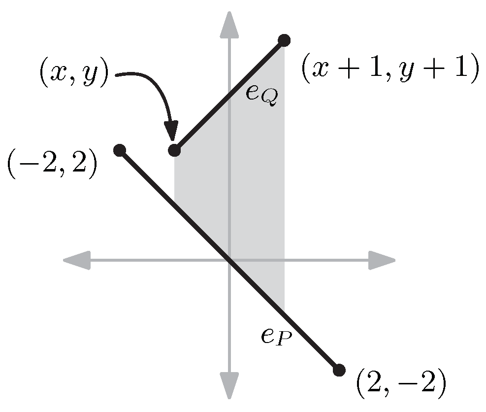
For each interval s of ${\mathcal{S}}_{\mathcal{T}}$, we find a vector $t_s\in s$ that minimizes $d_2$. For a vertex–edge pair $(v,e)$ where $v\in Q_c$ and $e\in P_c$, the set of all vectors $\tau \in {\mathbb{R}}^2$ is such that $v+\tau \in e$ forms a segment $e^{\prime }:=e\ominus v$. Moreover, for any vector ${\tau }^{\prime }$ lying above $e^{\prime }$, $v+{\tau }^{\prime }$ also lies above e and the vertical distance between ${\tau }^{\prime }$ and $e^{\prime }$ is the same as the vertical distance between $v+{\tau }^{\prime }$ and e. See Figure 4. Similarly, for a vertex–edge pair $(v,e)$ where $v\in P_c$ and $e\in Q_c$, any vector ${\tau }^{\prime }$ lying above $e^{\prime }:=v\ominus e$ makes v lie below $e+{\tau }^{\prime }$, and the vertical distance between ${\tau }^{\prime }$ and $e^{\prime }$ is the same as the vertical distance between v and $e+{\tau }^{\prime }$.

Figure 4. (left,middle) The pairs $(v+{\tau }^{\prime },e)$ and $({\tau }^{\prime },e^{\prime })$ have the same geometric configuration. (right) The red arrow is the minimum pointwise vertical distance between $U_s$ and $L_s$.

Let $E_s$ be a set of all segments $e^{\prime }$ computed as above for every pair $(v,e)$ in $C\left(t\right)$ for $t\in s$, and let $U_s$ and $L_s$ be the upper and lower envelopes of $E_s$ on s, respectively. From the same argument of Lemma 1, we observe $U_s\subset h\left[\mathcal{T}\right]$. Moreover, the scoring criterion $d_2\left(t\right)$ is the same as the vertical distance between $(t,h(t\left)\right)$ and $L_s$. Therefore, the vector $t_s\in s$ that minimizes the scoring criterion $d_2$ also minimizes the pointwise vertical distance between $U_s$ and $L_s$. See Figure 4.

Let $t_i\le t_{i+1}$ be the endpoints of the interval s. See every edge $e^{\prime }$ in $E_s$ that intersects the vertical lines $x=t_i$ and $x=t_{i+1}$. This implies that $U_s$ (resp. $L_s$) is a convex (resp. concave) piecewise linear curve of $O(m+n)$ complexity. Hence, we could find $t_s\in s$ in $O(logn+logm)$ time using binary search, once we compute $U_s$ and $L_s$.

Observe that the combinatorial structures corresponding to adjacent intervals in ${\mathcal{S}}_{\mathcal{T}}$ have only $O\left(1\right)$ different pairs. Herschberger and Suri [15] proposed an algorithm maintains the convex hull throughout the process of updating points in ${\mathbb{R}}^2$. More specifically, given an insert/delete sequence of points of length N, their algorithm maintains the convex hull using $O(NlogN)$ time and $O\left(N\right)$ space. With the point-line duality [10], we can maintain the upper and lower envelopes for a updating sequence of lines. We scan the intervals in ${\mathcal{S}}_{\mathcal{T}}$ from left to right, and compute the updating sequence of lines of length $O\left(mn\right)$, which corresponds to the changes in $C\left(t\right)$. By applying [15], we compute $U_s$ and $L_s$ corresponding to each interval s in ${\mathcal{S}}_{\mathcal{T}}$ in a total of $O\left(mn\right(logm+logn\left)\right)$ time.

We conclude this section with the following theorem, which analyzes the time and space complexities of finding the optimal translation vector.

Theorem 3.

Let P and Q be two y-monotone polygons in ${\mathbb{R}}^2$, such that $P_c$ and $Q_c$ have n and m vertices, respectively. The optimal placement of Q on top of P which minimizes the maximum pointwise vertical distance between $P_c$ and $Q_c$ can be computed in $O\left(mn\right(logm+logn\left)\right)$ time using $O\left(mn\right)$ space.

Proof. 

We subdivide $\mathcal{T}$ into ${\mathcal{S}}_{\mathcal{T}}$, such that the translation vectors belonging to the same interval of ${\mathcal{S}}_{\mathcal{T}}$ have the same combinatorial structure. This can be performed in $O\left(mn\right(logm+logn\left)\right)$ time, and the size of ${\mathcal{S}}_{\mathcal{T}}$ is $O\left(mn\right)$. The size of the combinatorial structure corresponding to an interval s of ${\mathcal{S}}_{\mathcal{T}}$ is $O(m+n)$, so the sizes of $U_s$ and $L_s$ are $O(m+n)$.

The vector that minimizes the vertical distance between $U_s$ and $L_s$ can be computed in $O(logm+logn)$ time by applying binary searches on $U_s$ and $L_s$.

When scanning the intervals in ${\mathcal{S}}_{\mathcal{T}}$ sequentially, we can maintain $U_s$ and $L_s$ in total $O\left(mn\right(logm+logn\left)\right)$ time. Therefore, we can find the optimal translation vector in $O\left(mn\right(logm+logn\left)\right)$ time using $O\left(mn\right)$ space. □

4.2. The Case When $d\ge 3$

Similarly to the case when $d=2$, we calculate the subdivision ${\mathcal{S}}_{\mathcal{T}}$ of $\mathcal{T}$ such that $C\left(t\right)$ remains the same for vectors t in a cell. Next, by traversing each cell of ${\mathcal{S}}_{\mathcal{T}}$, we update $C\left(t\right)$ and solve a linear programming problem to find the vector in the cell that minimizes $d_2$.

When $Q+h\left[t\right]$ is placed on top of P for $t\in \mathcal{T}$, the maximum pointwise vertical distance $Q_c+h\left[t\right]$ and $P_c$ is realized by a pair $(p_i,q_{d-i-1})$, such that $p_i$ is an i-face of $P_c$ and $q_{d-i-1}$ is a $(d-i-1)$-face of $Q_c$ for $0\le i\le d-1$ and $q_{d-i-1}+h\left[t\right]$ lies above $p_i$. Therefore, $C\left(t\right)$ becomes the set of pairs $(p_i,q_{d-i-1})$ that need to be considered to compute $d_2\left(t\right)$ for a vector $t\in \mathcal{T}$.

We calculate the subdivision ${\mathcal{S}}_{\mathcal{T}}$ of $\mathcal{T}$ based on whether $C\left(t\right)$ remains the same. $C\left(t\right)$ changes when a vertex of ${\mathbb{D}}_P$ starts or stops intersecting a face of ${\mathbb{D}}_Q+t$, or vice versa. Therefore, ${\mathcal{S}}_{\mathcal{T}}$ is the intersection of $\mathcal{T}$ with the overlay of m translated copies of ${\mathbb{D}}_P$ and n translated copies of ${\mathbb{D}}_Q$. Note that ${\mathbb{D}}_P$ and ${\mathbb{D}}_Q$ are triangulations of complexity $O\left(n^{\lfloor (d-1)/2\rfloor }\right)$ and $O\left(m^{\lfloor (d-1)/2\rfloor }\right)$, respectively [9]. Furthermore, $\mathcal{T}$ is the set of translation vectors that place every vertex of ${\mathbb{D}}_Q$ inside ${\mathbb{D}}_P$, so $\mathcal{T}$ can be described as common intersection of $O\left(n^{\lfloor (d-1)/2\rfloor }\right)$ half-spaces in ${\mathbb{R}}^{d-1}$. Hence, ${\mathcal{S}}_{\mathcal{T}}$ has a complexity of $O\left({\left(mn\right)}^{(d-1)\lfloor (d+1)/2\rfloor }\right)$, and can be computed in $O\left({\left(mn\right)}^{(d-1)\lfloor (d+1)/2\rfloor }\right)$ time [16,17]. When $d=3$, we could apply more efficient algorithm in [18], and compute ${\mathcal{S}}_{\mathcal{T}}$ with $O\left({\left(mn\right)}^2\right)$ time and space.

Let s be a cell in ${\mathcal{S}}_{\mathcal{T}}$. For a vector $t\in s$, the size of $C\left(t\right)$ is $O\left({\left(mn\right)}^{\lfloor (d-1)/2\rfloor }\right)$, since the number of faces in $P_c$ and $Q_c$ is $O\left(n^{\lfloor (d-1)/2\rfloor }\right)$ and $O\left(m^{\lfloor (d-1)/2\rfloor }\right)$, respectively. Let $(p_i,q_{d-i-1})$ be a pair of $C\left(t\right)$. The set of vectors $\tau \in {\mathbb{R}}^d$ that make $p_i$ and $q_{d-i-1}+\tau$ intersect is $p_i\ominus q_{d-i-1}$. Among these vectors, let $s(p_i,q_{d-i-1})$ denotes the set of vectors whose projection onto the plane $x_d=0$ lies in s. Let $E_s$ be the union of $s(p_i,q_{d-i-1})$ for all pairs in $C\left(t\right)$, and the upper and lower envelope of $E_s$ be $U_s$ and $L_s$, respectively. Same as the case when $d=2$, $U_s\subset h\left[\mathcal{T}\right]$ and the optimal vector of $t_s$ that minimizes $d_2$ realizes the minimum pointwise vertical distance between $U_s$ and $L_s$.

However, for dimensions $d\ge 3$, $t_s$ cannot be found through a simple binary search. For a pair $(p_i,q_{d-i-1})$ in $C\left(t\right)$, consider the $(d+1)$-dimensional points $(t,l,v_{(t,l)})$, where $t\in s$ and $l,v_{(t,l)}\in \mathbb{R}$, such that $v_{(t,l)}$ is the vertical distance between $p_i$ and $q_{d-i-1}+(t,l)$. The set of points $(t,l,v_{(t,l)})$ forms (a part of) a $(d+1)$-dimensional hyperplane. From the upper envelope of the hyperplanes formed for all pairs in $C\left(t\right)$ and $O\left({\left(mn\right)}^{\lfloor (d-1)/2\rfloor }\right)$, many additional hyperplanes that make $q_{d-i-1}$ lie above $p_i$, and the point with the smallest $x_{d+1}$-coordinate corresponds to the optimal vector $t_s$. Matoušek and Schwarzkopf [19] presented an algorithm for N hyperplanes in ${\mathbb{R}}^{d+1}$ such that, after $O\left(N^{1+{\displaystyle \frac{1+\delta -\lfloor (d+1)/2\rfloor }{1+\delta +\lfloor (d+1)/2\rfloor }}}\right)$ preprocessing time, one can insert or delete a hyperplane and find the point with the smallest $x_{d+1}$-coordinate in $O\left(N^{{\displaystyle \frac{1+\delta -\lfloor (d+1)/2\rfloor }{1+\delta +\lfloor (d+1)/2\rfloor }}}\right)$ time for a constant $\delta >0$. By traversing $O\left({\left(mn\right)}^{(d-1)\lfloor (d+1)/2\rfloor }\right)$ cells in ${\mathcal{S}}_{\mathcal{T}}$, we update hyperplanes and find the optimal vector in each cell in $O\left({\left(mn\right)}^{(d-1){\displaystyle \frac{1+\delta -\lfloor (d+1)/2\rfloor }{1+\delta +\lfloor (d+1)/2\rfloor }}}\right)$ time. When $d=3$, the size of $C\left(t\right)$ is $O(m+n)$, and we find the optimal vector in s in $O\left({\left(mn\right)}^{1/3+\delta }\right)$ time.

We conclude this section with the following theorem, which analyzes the time and space complexities of finding the optimal translation vector.

Theorem 4.

Let P and Q be two $x_d$-monotone polytopes in ${\mathbb{R}}^d$ for $d\ge 3$, such that $P_c$ and $Q_c$ have n and m vertices, respectively. For a constant $\delta >0$, the optimal placement of Q on top of P which minimizes the maximum pointwise vertical distance that can be computed in $O\left({\left(mn\right)}^{7/3+\delta }\right)$ time using $O\left({\left(mn\right)}^2\right)$ space for $d=3$, and in $O\left({\left(mn\right)}^{(d-1)\lfloor (d-1)/2\rfloor \lfloor (d+1)/2\rfloor {\displaystyle \frac{1+\delta -\lfloor (d+1)/2\rfloor }{1+\delta +\lfloor (d+1)/2\rfloor }}}\right)$ time and $O\left({\left(mn\right)}^{(d-1)\lfloor (d+1)/2\rfloor }\right)$ space for $d>3$.

Proof. 

We subdivide $\mathcal{T}$ into ${\mathcal{S}}_{\mathcal{T}}$, such that the translation vectors belonging to the same cell of ${\mathcal{S}}_{\mathcal{T}}$ have the same combinatorial structure. When $d=3$, this can be performed in $O\left({\left(mn\right)}^2\right)$ time and space, and when $d>3$, it can be performed in $O\left({\left(mn\right)}^{(d-1)\lfloor (d+1)/2\rfloor }\right)$ time and space.

The size of the combinatorial structure corresponding to a cell s of ${\mathcal{S}}_{\mathcal{T}}$ is $O\left({\left(mn\right)}^{\lfloor (d-1)/2\rfloor }\right)$, and we find the optimal translation vector in s by solving a linear programming problem in ${\mathbb{R}}^{d+1}$ with $O\left({\left(mn\right)}^{\lfloor (d-1)/2\rfloor }\right)$ constraints.

When traversing the cells in ${\mathcal{S}}_{\mathcal{T}}$ sequentially, using a data structure that supports the insertion and deletion of the constraints, we find the optimal translation vector in s in $O\left({\left(mn\right)}^{1/3+\delta }\right)$ time when $d=3$ or $O\left({\left(mn\right)}^{\lfloor (d-1)/2\rfloor {\displaystyle \frac{1+\delta -\lfloor (d+1)/2\rfloor }{1+\delta +\lfloor (d+1)/2\rfloor }}}\right)$ time when $d>3$. Therefore, we can find the optimal translation vector in $O\left({\left(mn\right)}^{7/3+\delta }\right)$ time using $O\left({\left(mn\right)}^2\right)$ space for $d=3$, and in $O\left({\left(mn\right)}^{(d-1)\lfloor (d-1)/2\rfloor \lfloor (d+1)/2\rfloor {\displaystyle \frac{1+\delta -\lfloor (d+1)/2\rfloor }{1+\delta +\lfloor (d+1)/2\rfloor }}}\right)$ time and $O\left({\left(mn\right)}^{(d-1)\lfloor (d+1)/2\rfloor }\right)$ space for $d>3$. □

5. Minimizing Scoring Criterion (3)

In this section, we demonstrate how to find the translation vector that minimizes the scoring criterion $d_3$.

5.1. The Case When $d=2$

When $Q+h\left[t\right]$ is placed on top of P for $t\in \mathcal{T}$, the scoring criterion $d_3$ measures the sum of the area between pairs of edges $(e_P,e_Q)$, such that $e_P\in P_c$, $e_Q\in Q_c$ and $e_Q+h\left[t\right]$ lies above $e_P$. Let $C\left(t\right)$ denotes the set of edge pairs that need to be considered to compute $d_3\left(t\right)$. We subdivide $\mathcal{T}$ into ${\mathcal{S}}_{\mathcal{T}}$ based on whether the combinatorial structure $C\left(t\right)$ are the same. As in Section 4.1, ${\mathcal{S}}_{\mathcal{T}}$ is defined as the overlay of m translated copies of ${\mathbb{D}}_P$ and m translated copies of ${\mathbb{D}}_Q$. Therefore, ${\mathcal{S}}_{\mathcal{T}}$ can be computed in $O\left(mn\right(logm+logn\left)\right)$ time and $O\left(mn\right)$ space. Also, the size of $C\left(t\right)$ is $O(m+n)$.

As we did in Section 4.1, we can sequentially compute $U_s$ corresponding to the intervals s of ${\mathcal{S}}_{\mathcal{T}}$ in $O\left(mn\right(logm+logn\left)\right)$ time and $O\left(mn\right)$ space. Let u be a segment of $U_s$. For vectors $\tau \in u$, the area between $e_Q+\tau$ and $e_P$ can be expressed as a constant degree polynomial. See Figure 5 as an example. Therefore, the area between $Q_c+\tau$ and $P_c$ can also be expressed as a constant degree polynomial. Consequently, the vector in u that minimizes the area between $Q_c+\tau$ and $P_c$ can be found in $O\left(1\right)$ time using a numerical method. The total number of segments in $U_s$ that apply this method is bounded by the complexity of $h\left[\mathcal{T}\right]$, which is $O\left(mn\alpha \right(mn\left)\right)$.

Figure 5. $e_Q$ lies above $e_P$, and $-2\le x\le 1$ where $(x,y)$ is the left endpoint of $e_Q$. The volume between $e_Q$ and $e_P$ is $0.5x+1.5y+1$.

We conclude this section with the following theorem, which analyzes the time and space complexities of finding the optimal translation vector.

Theorem 5.

Let P and Q be two y-monotone polygons in ${\mathbb{R}}^2$, such that $P_c$ and $Q_c$ have n and m vertices, respectively. The optimal placement of Q on top of P which minimizes the volume between $P_c$ and $Q_c$ can be computed in $O\left(mn\right(logm+logn\left)\right)$ time using $O\left(mn\right)$ space.

Proof. 

We subdivide $\mathcal{T}$ into ${\mathcal{S}}_{\mathcal{T}}$, such that the translation vectors belonging to the same interval of ${\mathcal{S}}_{\mathcal{T}}$ have the same combinatorial structure. This can be performed in $O\left(mn\right(logm+logn\left)\right)$ time, and the size of ${\mathcal{S}}_{\mathcal{T}}$ is $O\left(mn\right)$. The size of the combinatorial structure corresponding to an interval s of ${\mathcal{S}}_{\mathcal{T}}$ is $O(m+n)$, so the sizes of $U_s$ is $O(m+n)$.

For an interval s of ${\mathcal{S}}_{\mathcal{T}}$, the vector $t_s\in s$ that minimizes the volume between $P_c$ and $Q_c+t_s$ can be computed in $O\left(1\right)$ time, once we have the function corresponding to the volume between $P_c$ and $Q_c+t_s$.

When scanning the intervals in ${\mathcal{S}}_{\mathcal{T}}$ sequentially, we compute $U_{s_0}$ for the first interval $s_0$ of ${\mathcal{S}}_{\mathcal{T}}$ and the volume function for the first segment of $U_{s_0}$ in $O\left(\right(m+n\left)\right(logm+logn\left)\right)$ time. For the remaining intervals, we can maintain $U_s$ and the volume function in total $O\left(mn\right(logm+logn\left)\right)$ time. Therefore, we can find the optimal translation vector in $O\left(mn\right(logm+logn\left)\right)$ time using $O\left(mn\right)$ space. □

5.2. The Case When $d\ge 3$

Similarly to the case when $d=2$, we calculate the subdivision ${\mathcal{S}}_{\mathcal{T}}$ of $\mathcal{T}$ such that $C\left(t\right)$ remains the same. Next, by traversing each cell s in ${\mathcal{S}}_{\mathcal{T}}$, we compute $h\left[\mathcal{T}\right]$ on s and find the vector minimizing the volume between $Q_c+\tau$ and $P_c$.

When $Q+h\left[t\right]$ is placed on top of P for $t\in \mathcal{T}$, the scoring criterion $d_3$ measures the sum of the area between pairs of $(d-1)$-faces $(e_P,e_Q)$, such that $e_P\in P_c$, $e_Q\in Q_c$ and $e_Q+h\left[t\right]$ lies above $e_P$. Let $C\left(t\right)$ denotes the set of $(d-1)$-face pairs that need to be considered to compute $d_3\left(t\right)$. We subdivide $\mathcal{T}$ into ${\mathcal{S}}_{\mathcal{T}}$ based on whether the combinatorial structure $C\left(t\right)$ are the same. As we did in Section 4.2, ${\mathcal{S}}_{\mathcal{T}}$ is defined as the overlay of m translated copies of ${\mathbb{D}}_P$ and m translated copies of ${\mathbb{D}}_Q$ within $\mathcal{T}$. Hence, ${\mathcal{S}}_{\mathcal{T}}$ has a complexity of $O\left({\left(mn\right)}^{(d-1)\lfloor (d+1)/2\rfloor }\right)$, and can be computed in $O\left({\left(mn\right)}^{(d-1)\lfloor (d+1)/2\rfloor }\right)$ time [16,17] for $d>3$, and $O\left({\left(mn\right)}^2\right)$ time and space [18] for $d=3$.

For a cell s in ${\mathcal{S}}_{\mathcal{T}}$, consider the pair $(e_P,e_Q)$ in $C\left(t\right)$ for $t\in s$. For any face k in the triangulation of $h\left[s\right]$, the volume between $e_Q+\tau$ and $e_P$ for $\tau \in k$ can be expressed as a constant degree polynomial. Therefore, the volume between $Q_c+\tau$ and $P_c$ can also be expressed as a constant degree polynomial, and the vector in k that minimizes the volume can be calculated in $O\left(1\right)$ time using numerical methods. Since $h\left[s\right]$ is the upper envelope on s of $O\left({\left(mn\right)}^{\lfloor (d-1)/2\rfloor }\right)$ hyperplanes in ${\mathbb{R}}^d$ corresponding to the i-face and $(d-i-1)$-face pairs of $P_c$ and $Q_c$, it can be computed in $O({\left(mn\right)}^{\lfloor d/2\rfloor \lfloor (d-1)/2\rfloor }+mn(logm+logn))$ time [20]. Similarly, the triangulation of s can be computed within the same time and space complexity.

We conclude this section with the following theorem, which analyzes the time and space complexities of finding the optimal translation vector.

Theorem 6.

Let P and Q be two $x_d$-monotone polygons in ${\mathbb{R}}^d$ for $d\ge 3$, such that $P_c$ and $Q_c$ have n and m vertices, respectively. The optimal placement of Q on top of P which minimizes the volume between $P_c$ and $Q_c$ can be computed in $O\left({\left(mn\right)}^{(d-1)\lfloor (d-1)/2\rfloor \lfloor d/2\rfloor \lfloor (d+1)/2\rfloor }\right)$ time and space.

Proof. 

We subdivide $\mathcal{T}$ into ${\mathcal{S}}_{\mathcal{T}}$, such that the translation vectors belonging to the same cell of ${\mathcal{S}}_{\mathcal{T}}$ have the same combinatorial structure. This can be performed in $O\left({\left(mn\right)}^{(d-1)\lfloor (d+1)/2\rfloor }\right)$ time and space. The size of the combinatorial structure corresponding to a cell s of ${\mathcal{S}}_{\mathcal{T}}$ is $O\left({\left(mn\right)}^{\lfloor (d-1)/2\rfloor }\right)$. Hence, we can compute the graph $h\left[s\right]$ in $O({\left(mn\right)}^{\lfloor d/2\rfloor \lfloor (d-1)/2\rfloor }+mn(logm+logn))$ time.

For a face k in $h\left[s\right]$, we can find the optimal translation vector in k in $O\left(1\right)$ time, once we have the function corresponding to the volume between $P_c$ and $Q_c+t_k$ for $t_k\in k$. The volume function can be computed in $O\left({\left(mn\right)}^{\lfloor (d-1)/2\rfloor }\right)$ time for the first face $k_0$ of $h\left[s\right]$, and then updated in $O\left(1\right)$ time along any (continuous) traversal order of the faces of $h\left[s\right]$ from $k_0$. Therefore, we can find the optimal translation vector in $O\left({\left(mn\right)}^{(d-1)\lfloor (d-1)/2\rfloor \lfloor d/2\rfloor \lfloor (d+1)/2\rfloor }\right)$ time and space. □

6. Discussion and Conclusions

In this paper, we propose algorithms to find the optimal location of Q on top of P under three different scoring criteria. The proposed algorithms are based on a detailed analysis of the geometric configurations and the careful application of suitable data structures. More specifically, the vector minimizing $d_1$ is computed by finding the point with the minimum $x_d$-coordinate in the graph $h\left[\mathcal{T}\right]$. To find the vector minimizing $d_2$, we first subdivide $\mathcal{T}$ into ${\mathcal{S}}_{\mathcal{T}}$ such that the combinatorial structure remains the same in a cell of ${\mathcal{S}}_{\mathcal{T}}$. Then, we find the optimal vector in s by solving a linear programming (LP) problem, and we also improve the time complexity by applying data structures that support constraint updates, leveraging the similarity of the LP problems corresponding to each cell. To find the vector minimizing $d_3$, we use the same subdivision ${\mathcal{S}}_{\mathcal{T}}$ as in the case for $d_2$. For each cell $s\in {\mathcal{S}}_{\mathcal{T}}$, the volume function between $P_c$ and $Q_c+\tau$ for $\tau \in h\left[s\right]$ is expressed as a constant degree polynomial when $\tau$ is restricted in a face of $h\left[s\right]$ that has non-zero volume. Hence, we explicitly compute $h\left[s\right]$ and find the optimal vector in each face of $h\left[s\right]$ using numerical methods.

We expect that a careful implementation of the algorithm proposed in this paper can be applied to various real-world applications. Additionally, if the input polytope is composed of triangles that satisfy conditions such as “fat” [21], we anticipate that the calculation of the optimal stacking can be performed more efficiently in practice than the worst-case analysis presented in this paper.

Future research may extend to cases where ${\mathbb{D}}_P$ and ${\mathbb{D}}_Q$ are non-convex, where P and Q are not $x_d$-monotone, where P and Q have symmetry, or where both translation and rotation are considered. We expect that the algorithms presented in this paper will serve as a solid baseline for these diverse follow-up studies.

References

- Kepler, J. The Six-Cornered Snowflake; Paul Dry Books: Philadelphia, PA, USA, 2010. [Google Scholar]
- Paterson, M.; Peres, Y.; Thorup, M.; Winkler, P.; Zwick, U. Maximum overhang. Am. Math. Mon. 2009, 116, 763–787. [Google Scholar] [CrossRef]
- Lee, S.J. Efficient Algorithms for Stacking Polytopes. Master’s Thesis, Pohang University of Science and Technology, Pohang, Republic of Korea, 2019. [Google Scholar]
- Ahn, H.K.; Abardia, J.; Bae, S.W.; Cheong, O.; Dann, S.; Park, D.; Shin, C.S. The minimum convex container of two convex polytopes under translations. Comput. Geom. 2019, 77, 40–50. [Google Scholar] [CrossRef]
- Egeblad, J.; Nielsen, B.K.; Brazil, M. Translational packing of arbitrary polytopes. Comput. Geom. 2009, 42, 269–288. [Google Scholar]
- Trivella, A.; Pisinger, D. Bin-Packing Problems with Load Balancing and Stability Constraints. In Proceedings of the INFORMS Transportation and Logistics Society, Chicago, IL, USA, 26–29 July 2017. [Google Scholar]
- Casko, J.S.; Vaden, J.L.; Kokich, V.G.; Damone, J.; James, R.D.; Cangialosi, T.J.; Riolo, M.L.; Owens, S.E.; Bills, E.D. Objective grading system for dental casts and panoramic radiographs. Am. J. Orthod. Dentofac. Orthop. 1998, 114, 589–599. [Google Scholar] [CrossRef] [PubMed]
- Hershberger, J. Finding the upper envelope of n line segments in O(n log n) time. Inf. Process. Lett. 1989, 33, 169–174. [Google Scholar] [CrossRef]
- McMullen, P. The maximum numbers of faces of a convex polytope. Mathematika 1970, 17, 179–184. [Google Scholar] [CrossRef]
- Berg, M.; Cheong, O.; Kreveld, M.; Overmars, M. Computational Geometry: Algorithms and Applications; Springer Science & Business Media: Berlin/Heidelberg, Germany, 2000. [Google Scholar]
- Dobkin, D.P.; Kirkpatrick, D.G. A linear algorithm for determining the separation of convex polyhedra. J. Algorithms 1985, 6, 381–392. [Google Scholar] [CrossRef]
- Dobkin, D.P.; Kirkpatrick, D.G. Determining the separation of preprocessed polyhedra—A unified approach. In International Colloquium on Automata, Languages, and Programming; Springer: Berlin/Heidelberg, Germany, 1990; pp. 400–413. [Google Scholar]
- Edelsbrunner, H.; Guibas, L.J.; Sharir, M. The upper envelope of piecewise linear functions: Algorithms and applications. Discret. Comput. Geom. 1989, 4, 311–336. [Google Scholar] [CrossRef]
- Agarwal, P.K.; Aronov, B.; Sharir, M. Computing envelopes in four dimensions with applications. In Proceedings of the Tenth Annual Symposium on Computational Geometry, Stony Brook, NY, USA, 6–8 June 1994; pp. 348–358. [Google Scholar]
- Herschberger, J.; Suri, S. Offline maintenance of planar configurations. In Proceedings of the Second Annual ACM-SIAM Symposium on Discrete Algorithms, San Francisco, CA, USA, 28–30 January 1991; pp. 32–41. [Google Scholar]
- Clarkson, K.L. New applications of random sampling in computational geometry. Discret. Comput. Geom. 1987, 2, 195–222. [Google Scholar] [CrossRef][Green Version]
- Edelsbrunner, H.; O’Rourke, J.; Seidel, R. Constructing arrangements of lines and hyperplanes with applications. Siam J. Comput. 1986, 15, 341–363. [Google Scholar] [CrossRef]
- Balaban, I.J. An optimal algorithm for finding segments intersections. In Proceedings of the Eleventh Annual Symposium on Computational Geometry, Vancouver, BC, Canada, 5–7 June 1995; pp. 211–219. [Google Scholar]
- Matoušek, J.; Schwarzkopf, O. Linear optimization queries. In Proceedings of the Eighth Annual Symposium on Computational Geometry, Berlin, Germany, 10–12 June 1992; pp. 16–25. [Google Scholar]
- Chazelle, B. An optimal convex hull algorithm in any fixed dimension. Discret. Comput. Geom. 1993, 10, 377–409. [Google Scholar] [CrossRef]
- Moet, E.; van Kreveld, M.; der Stappen, A.F.v. On realistic terrains. Comput. Geom. 2008, 41, 48–67. [Google Scholar] [CrossRef][Green Version]
Disclaimer/Publisher’s Note: The statements, opinions and data contained in all publications are solely those of the individual author(s) and contributor(s) and not of MDPI and/or the editor(s). MDPI and/or the editor(s) disclaim responsibility for any injury to people or property resulting from any ideas, methods, instructions or products referred to in the content. |
© 2024 by the authors. Licensee MDPI, Basel, Switzerland. This article is an open access article distributed under the terms and conditions of the Creative Commons Attribution (CC BY) license (https://creativecommons.org/licenses/by/4.0/).