Article

Three-Dimensional Moran Walk with Resets

by
Mohamed Abdelkader
Department of Statistics and Operations Research, King Saud University, Riyadh 11451, Saudi Arabia
Symmetry 2024, 16(9), 1222; https://doi.org/10.3390/sym16091222
Submission received: 10 May 2024 / Revised: 7 September 2024 / Accepted: 11 September 2024 / Published: 18 September 2024
(This article belongs to the Section Mathematics)

Abstract

:
In this current paper, we propose to study a three-dimensional Moran model ( X n ( 1 ) , X n ( 2 ) , X n ( 3 ) ) , where each random walk ( X n ( i ) ) { 1 , 2 , 3 } increases by one unit or is reset to zero at each unit of time. We analyze the joint law of its final altitude X n = max ( X n ( 1 ) , X n ( 2 ) , X n ( 3 ) ) via the moment generating tools. Furthermore, we show that the limit distribution of each random walk follows a shifted geometric distribution with parameter 1 q i , and we analyze the maximum of these three walks, also giving explicit expressions for the mean and variance.

1. Introduction

In this study, we consider a discrete random walk with three dimensions ( X n ( 1 ) , X n ( 2 ) , X n ( 3 ) ) , defined as follows: our walk starts from the origin at time (0, 0, 0). At each time step, the walk moves by one positive unit in the direction of the x-axis (1, 0, 0) with probability p 2 ; in the direction of the y-axis (0, 1, 0) with probability p 3 ; or in the direction of the z-axis (0, 0, 1) with probability p 4 . Or, it resets to (0, 0, 0) with probability p 1 , or shifts one unit in all three directions (1, 1, 1) with probability p 5 such that p 1 + p 2 + p 3 + p 4 + p 5 = 1 . Here are some examples illustrating the evolution of our model:
( 0 , 0 , 0 ) p 3 ( 0 , 1 , 0 ) p 2 ( 1 , 0 , 0 ) p 5 ( 2 , 1 , 1 ) p 5 ( 3 , 2 , 2 ) p 4 ( 0 , 0 , 3 ) p 1 ( 0 , 0 , 0 ) ,
( 0 , 0 , 0 ) p 2 ( 1 , 0 , 0 ) p 2 ( 2 , 0 , 0 ) p 5 ( 3 , 1 , 1 ) p 1 ( 0 , 0 , 0 ) p 4 ( 0 , 0 , 1 ) p 4 ( 0 , 0 , 2 ) ,
( 0 , 0 , 0 ) p 4 ( 0 , 0 , 1 ) p 5 ( 1 , 1 , 2 ) p 4 ( 0 , 0 , 3 ) p 5 ( 1 , 1 , 4 ) p 5 ( 2 , 2 , 5 ) p 5 ( 3 , 3 , 6 ) ,
( 0 , 0 , 0 ) p 5 ( 1 , 1 , 1 ) p 5 ( 2 , 2 , 2 ) p 3 ( 0 , 3 , 0 ) p 1 ( 0 , 0 , 0 ) p 5 ( 1 , 1 , 1 ) p 2 ( 2 , 0 , 0 ) ,
The final altitude of the random walks with a length 7 in the above examples are 0, 2, 6 and 2, respectively.
In this current paper, our goals are twofold: we will analyze the statistical properties of the final altitude denoted by X n max ( X n ( 1 ) , X n ( 2 ) , X n ( 3 ) ) by utilizing the moment-generating function (MGF) to derive its mean and variance. We will also examine the limit distribution, as well as the mean and variance, of each random walk X n ( i ) , i = 1 , 2 , 3 .
Numerous studies have explored the statistical properties of discrete random walks in one and higher dimensions using tools such as moment-generating functions, kernel methods, and singularity analysis (see [1,2,3]). For example, in one dimension, if one concentrates on articles which play a role in our study, Abdelkader and Aguech determined the cumulative function of the height, the mean and the variance of the final altitude in the Moran random walk with reset and short memory in [4]. Furthermore, Banderier and Nicodème studied the height for bounded discrete walks and proved that the height of bridges is converged to a Rayleigh limit law asymptotically in [5]. Additionally, Aguech, Althagafi, and Banderier analyzed the properties of the final altitude for the Moran random walk with one dimension in [6]. Finally, Banderier and Wallner investigated some statistics like the number of catastrophes for lattice paths with catastrophes in [7].
In higher dimensions, Althagafi and Abdelkader demonstrated that the age of each component follows a shifted geometric distribution asymptotically, and they derived the mean and the variance of the final altitude using the moment-generating function in the two-dimensional Moran model [8]. Additionally, Itoh, Mahmoud, and Takahashi showed that the stationary distribution is a convolution of geometric random variables and derived important results regarding normal distribution in soliton physics for wave propagation [9]. Aguech, Althagafi, and Banderier investigated various Moran models and proved that the heights of these walks asymptotically follow a discrete Gumbel distribution [6]. Other relevant articles discuss the Moran process [10,11].
The study of three-dimensional random walks is significant and new, as it investigates random walks with non-uniform initial probabilities ( p 2 p 3 p 4 ) , partially generalizing the results of Itoh and Mahmoud in [12] (which focused on random walks with uniform probabilities in any dimension). Furthermore, it extends the work of Althagafi and Abdelkader [8], in which the authors studied the final altitude for the two-dimensional random walk. Additionally, the results concerning the mean and the variance of the final altitude for the three-dimensional random walk generalize Theorem 2 in [6]. This study also provides insights into the general case of systems composed of n components with non-uniform initial probabilities ( p 2 p 3 p n ) .
The analysis of the final altitude of random walks has broad applications across various fields, as random walks are widely used to model complex problems. For instance, Moran walks model mutation transmission in genetics [12,13,14], and they have applications in graph theory [15]. Additionally, random walks contribute to physics, such as the soliton wave model [9], which describes a stochastic system of particles representing a unidirectional wave. The final altitude is also relevant for estimating maximum electricity consumption and reservoir water levels.
The structure of this current paper is organized as follows. In Section 2, we describe our Moran random walk with three dimensions. In Section 3, we state our main result concerning the statistical properties such as the mean and the variance of the final altitude using the moment-generating function. In Section 4, we simulate the final altitude and the height statistics of our random walk using the R-program. In Section 5, we explore recursive equations relating the sequences of multivariate polynomials f n ( x 1 , x 2 , x 3 ) and f n 1 ( x 1 , x 2 , x 3 ) at two consecutive times n 1 and n using the recursive equations between P n ( s 1 , s 2 , s 3 ) and P n 1 ( s 1 , s 2 , s 3 ) . In Section 6, we show that the three random walks X n ( 1 ) , X n ( 2 ) , and X n ( 3 ) converge to geometric distribution asymptotically. Also, we establish the explicit expressions of their means and variances via the moment-generating function tool. In Section 7, we prove our main results. Finally, in Section 8, we present the conclusions of this work and we put forth some ideas for the next work.

2. Definitions and Presentation of the Model

We start by some definitions and present our model the three-dimensional random walks.

2.1. Definitions

  • Let ( U n , V n , W n ) { n = 0 , 1 , 2 , } be a discrete walk with three dimensions with ( U 0 , V 0 , W 0 ) = ( 0 , 0 , 0 ) and { 0 , 1 , , n } 3 the finite state space.
  • We define the probability associated to the discrete process ( U n , V n , W n ) for all k , r , s N by
    P n ( k , r , s ) = P ( U n = k , V n = r , W n = s ) .
  • The probability-generating function of a discrete variable Y, is given by: k 0
    G Y ( y ) = k = 0 y k P ( Y = k ) ,
    for all y R such that | y | < 1 , where P ( Y = k ) is the distribuation of a discrete variable Y.
We present the two following important relations concerning the link between the mean and the variance of a discrete random variable Y and its moment-generating function G Y ( y ) by:
E Y = G Y ( y ) y | y = 1 a n d V a r Y = 2 G Y ( y ) 2 y | y = 1 + E Y E Y 2 ,
where E Y and V a r Y represent the mean and the variance of Y.

2.2. Presentation of the Model

We consider the three-dimensional Moran model with three dimensions ( X n ( 1 ) , X n ( 2 ) , X n ( 3 ) ) , where the walk X n ( i ) represents the age of component i. It starts at time zero, with three components of age 0 days (i.e., ( X 0 ( 1 ) , X 0 ( 2 ) , X 0 ( 3 ) = ( 0 , 0 , 0 ) ), parameterized by five probabilities, denoted by p i , 1 i 5 .
( X n ( 1 ) , X n ( 2 ) , X n ( 3 ) ) = ( 0 , 0 , 0 ) , with p 1 , ( X n 1 ( 1 ) + 1 , 0 , 0 ) , with p 2 , ( 0 , X n 1 ( 2 ) + 1 , 0 ) , with p 3 , ( 0 , 0 , X n 1 ( 3 ) + 1 ) , with p 4 , ( X n 1 ( 1 ) + 1 , X n 1 ( 2 ) + 1 , X n 1 ( 3 ) + 1 ) , with p 5 ,
where p i ( 0 , 1 ) for 1 i 5 such that i = 1 5 p i = 1 . The final altitude X n and the height H n given by
X n = max ( X n ( 1 ) , X n ( 2 ) , X n ( 3 ) ) H n = max ( X 1 , , X n ) .
We denote by μ i , n , μ n , σ n 2 , and σ i , n 2 the means and the variances of X n ( i ) , i = 1 , 2 , 3 , and X n , respectively.

3. Main Result

In this section, we find the explicit expression of the probability-generating function of X n , denoted by Φ n ( u ) . Also, we derive Φ n ( u ) to establish the mean and the variance of X n . The function Φ n ( u ) is defined by: u R , i { 1 , 2 , 3 }
Φ n ( u ) = Φ X n ( u ) = k = 0 n u k P ( X n = k ) = k = 0 n u k P max ( X n ( 1 ) , X n ( 2 ) , X n ( 3 ) ) = k .
The next theorem present the closed form of the function Φ n ( u ) of X n . It is used to obtain the mean and the variance of the walk X n .
Theorem 1. 
The probability-generating function Φ n ( x ) of the final altitude is given by the following: for all n N * , u R ,
Φ n ( u ) = p 1 1 p 5 n u n 1 p 5 u + i = 1 3 ( ( q i u ) n ( 1 q i ) ( q i n p 5 n ) u n 1 q i u + p i + 1 ( 1 q i ) 1 q i u u p 5 n u n + 1 1 p 5 u ) .
where q i = p i + 1 + p 5 , | q i u | < 1 and | p 5 u | < 1 .
From Theorem 1, We deduce the mean and the variance of X n .
Theorem 2. 
The mean and the variance of X n are given by
μ n = q 1 q 1 n + 1 1 q 1 + q 2 q 2 n + 1 1 q 2 + q 3 q 3 n + 1 1 q 3 2 ( p 5 p 5 n + 1 ) 1 p 5 ,
and
σ n 2 = σ 1 2 + σ 2 2 + σ 3 2 + G n , p 5 + G n , q i , p 5 ,
where
G n , p 5 = 4 n p 5 n + 1 1 p 5 4 p 5 2 ( 1 p 5 n ) ( 1 p 5 ) 2 2 ( p 5 p 5 n + 1 ) 1 p 5 4 p 5 p 5 n + 1 1 p 5 2 ,
G n , q i , p 5 = 4 i = 1 3 q i q i n + 1 1 q i p 5 p 5 n + 1 1 p 5 2 i = 1 2 j = i + 1 3 q i q i n + 1 1 q i q j q j n + 1 1 q j ,
such that q i = p i + 1 + p 5 for i { 1 , 2 , 3 } .
Comments 1. 
We have the following special cases.
  • The expressions of μ n and σ n 2 in Equations (5) and (6) generalize the expressions of the mean and the variance in Theorem 2.1 in [6] for the one-dimensional random walks. Precisely, if we take our model (1), the probability p 4 = p 3 = p 2 = 0 , which means q 1 = q 2 = q 3 = p 5 . We start by the closed expression of the mean
    μ n = q 1 q 1 n + 1 1 q 1 + q 2 q 2 n + 1 1 q 2 + q 3 q 3 n + 1 1 q 3 2 ( p 5 p 5 n + 1 ) 1 p 5 = p 5 p 5 n + 1 1 p 5 + P 5 p 5 n + 1 1 p 5 + p 5 p 5 n + 1 1 q 3 2 ( p 5 p 5 n + 1 ) 1 p 5 = p 5 ( 1 p 5 n ) 1 p 5 .
    Taking q 2 = q 3 = q 4 = p 5 in Equation (6), we have
    G n , p 5 = 4 n p 5 n + 1 1 p 5 4 p 5 2 ( 1 p 5 n ) ( 1 p 5 ) 2 2 ( p 5 p 5 n + 1 ) 1 p 5 4 p 5 p 5 n + 1 1 p 5 2 = p 5 ( 1 p 5 ) 2 ( 4 n p 5 n ( 1 p 5 ) + 12 p 5 n + 1 8 p 5 2 ( 1 p 5 ) + 2 ( 1 p 5 ) p 5 n 4 p 5 2 n + 1 ) ,
    and
    G n , q i , p 5 = 4 i = 1 3 q i q i n + 1 1 q i p 5 p 5 n + 1 1 p 5 2 i = 1 2 j = i + 1 3 q i q i n + 1 1 q i q j q j n + 1 1 q j = 12 p 5 p 5 n + 1 1 p 5 2 6 p 5 p 5 n + 1 1 p 5 2 = 6 p 5 p 5 n + 1 1 p 5 2 .
    From Equation (28), we have
    σ 1 , n 2 = σ 2 , n 2 = σ 3 , n 2 = 2 n p 5 n + 1 ( 1 p 5 ) + 2 p 5 2 ( 1 p 5 n ) ( 1 p 5 ) 2 + p 5 p 5 n + 1 ( 1 p 5 ) p 5 p 5 n + 1 1 p 5 2 .
    and combining Equations (6) and (10)(12), we obtain
    σ n 2 = 2 n p 5 n + 1 ( 1 p 5 ) + 2 p 5 2 ( 1 p 5 n ) ( 1 p 5 ) 2 + p 5 p 5 n + 1 ( 1 p 5 ) p 5 p 5 n + 1 1 p 5 2 = p 5 ( 1 p 5 ) 2 1 p 5 n p 5 n + 1 + ( 1 + 2 n ) ( 1 p 5 ) .
    Equations (9) and (13) are the same as the expressions of the mean and the variance in Theorem 2.1 in [6] (taking p = p 5 and q = p 1 = 1 p 5 ).
  • The expressions of μ n and σ n 2 in Equations (5) and (6) generalize the expressions of the mean and the variance in Theorem 2 in [8]. Precisely, if we take our model (1), the probability p 4 equals 0, which means q 3 = p 4 + p 5 = p 5 . We start by the closed expression of the mean
    μ n = q 1 q 1 n + 1 1 q 1 + q 2 q 2 n + 1 1 q 2 + q 3 q 3 n + 1 1 q 3 2 ( p 5 p 5 n + 1 ) 1 p 5 = q 1 q 1 n + 1 1 q 1 + q 2 q 2 n + 1 1 q 2 + p 5 p 5 n + 1 1 q 3 2 ( p 5 p 5 n + 1 ) 1 p 5 = q 1 q 1 n + 1 1 q 1 + q 2 q 2 n + 1 1 q 2 p 5 p 5 n + 1 1 p 5 .
    Taking q 4 = p 5 in Equations (7) and (32), we have
    G n , q i , p 5 = 4 i = 1 3 q i q i n + 1 1 q i p 5 p 5 n + 1 1 p 5 2 i = 1 2 j = i + 1 3 q i q i n + 1 1 q i q j q j n + 1 1 q j = 4 p 5 p 5 n + 1 1 p 5 2 + 2 p 5 p 5 n + 1 1 p 5 q 1 q 1 n + 1 1 q 1 + 2 p 5 p 5 n + 1 1 p 5 q 2 q 2 n + 1 1 q 2 2 q 1 q 1 n + 1 1 q 1 q 2 q 2 n + 1 1 q 2 ,
    and
    σ 3 , n 2 = 2 n p 5 n + 1 ( 1 p 5 ) + 2 p 5 2 ( 1 p 5 n ) ( 1 p 5 ) 2 + p 5 p 5 n + 1 ( 1 p 5 ) p 5 p 5 n + 1 1 p 5 2 .
    Using Equation (7), we have
    G n , p 5 + 4 p 5 p 5 n + 1 1 p 5 2 = 4 n p 5 n + 1 1 p 5 4 p 5 2 ( 1 p 5 n ) ( 1 p 5 ) 2 2 ( p 5 p 5 n + 1 ) 1 p 5 .
    Combining Equations (16) and (17), we obtain
    σ 3 , n 2 + G n , p 5 + 4 p 5 p 5 n + 1 1 p 5 = 2 n p 5 n + 1 ( 1 p 5 ) 2 p 5 2 ( 1 p 5 n ) ( 1 p 5 ) 2 p 5 p 5 n + 1 ( 1 p 5 ) p 5 p 5 n + 1 1 p 5 2 = A p 5 .
    where A p 5 , is the correct formula defined when p 5 = p in (p. 20 in [8]). The authors in [8] forgot the following term p p n + 1 ( 1 p ) in the formula A p (p. 20 in [8]).
  • Finally, if p 4 = 0 , we have
    σ n 2 = σ 1 , n 2 + σ 2 , n 2 + A p 5 + 2 p 5 p 5 n + 1 1 p 5 q 1 q 1 n + 1 1 q 1 + 2 p 5 p 5 n + 1 1 p 5 q 2 q 2 n + 1 1 q 2 2 q 1 q 1 n + 1 1 q 1 q 2 q 2 n + 1 1 q 2 ,
    Equations (14) and (19) are the same as the expression of the mean and the variance for the two-dimensional Moran walk in [8] when q 1 = r 1 , q 2 = r 2 , p 5 = p , and p 1 = p 0 .
Remark 1. 
  • G n , p 5 and G n , q i , p 5 are two probabilities such that G n , p 5 depends only on the initial probability p 5 but G n , q i , p 5 depends on the initial probabilities ( p i ) i { 1 , 2 , 3 , 4 , 5 } .
  • Since X n = max ( X n ( 1 ) , X n ( 2 ) , X n ( 3 ) ) , then X n X n ( i ) , for i = 1 , 2 , 3 . So we deduce from Theorem 2 and Corollary 1 that E X n E X n ( i ) .

4. Application and Simulations

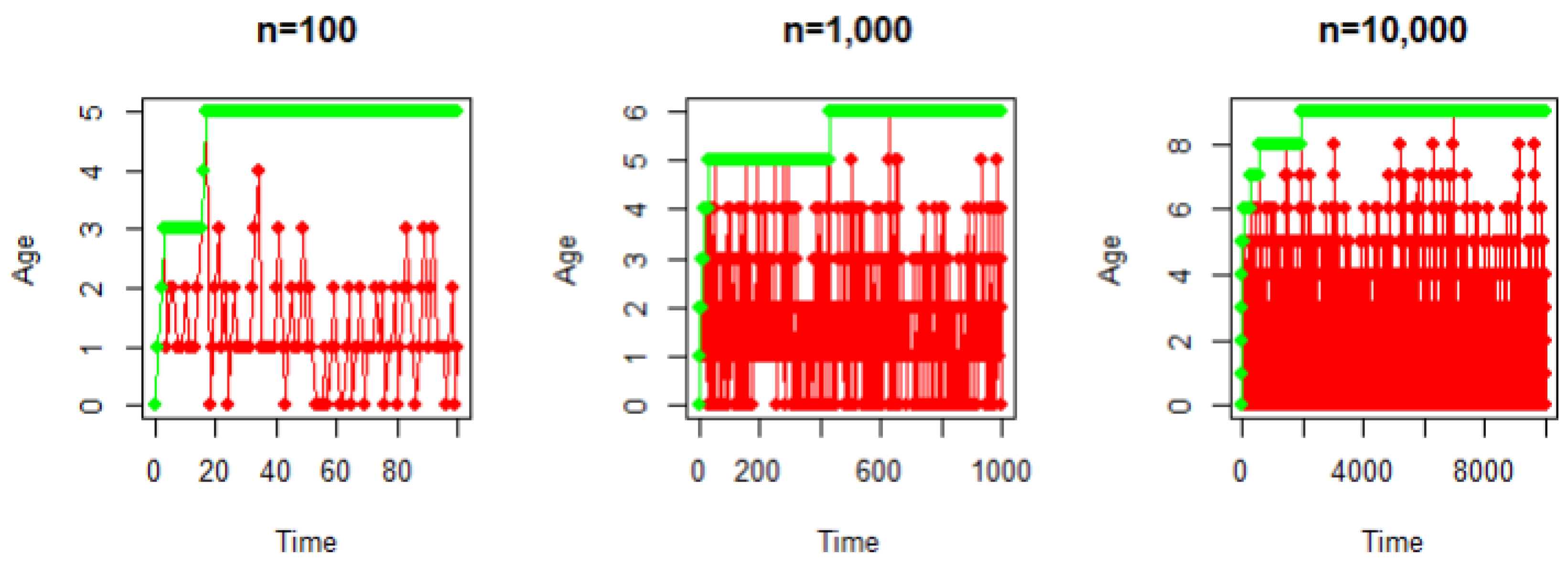
We present an application of our model. Also, we simulate the two walks X n and H n in the uniform ( p 1 = p 2 = p 3 = p 4 = p 5 = 1 / 5 ) and non-uniform ( p 1 = p 5 = 1 / 8 and p 2 = p 3 = p 4 = 1 / 4 or p 1 = 1 / 15 , p 2 = 2 / 8 , p 3 = 3 / 15 , p 4 = 4 / 15 and p 5 = 1 / 3 ) cases for n (100; 1000 and 10,000).

4.1. Application

In the three-dimensional Moran walk, consider a triplet of death gametes (representing par (0, 0, 0) at time 0 or in generation 0) with ages X ( 1 ) , X ( 2 ) and X ( 3 ) , who evolve in time. In generation k, the number of gametes is 5 k . The rules of the evolution are stochastic: at each time step k, a triplet of gametes are selected randomly. In the next generation k + 1 , the evolution of gametes is non-uniform (non-equally likely): the first gamete moves by one positive unit (survive gamete) and the others are deaths (1, 0, 0) with probability p 2 ; the second gamete is survive and the others are deaths (0, 1, 0) with probability p 3 ; the third gamete is survive and the others are deaths (0, 0, 1) with probability p 4 ; all are deaths (0, 0, 0) with probability p 1 ; or there is a shift of one unit in all three gametes (1, 1, 1) with probability p 5 such that p 1 + p 2 + p 3 + p 4 + p 5 = 1 . The unit of time is one year. We can refer to [12] for more details.
Let X n ( i ) , be the age of individual i = 1 , 2 , 3 in the Moran model at the nth generation n. Applying Theorem 3 and Corollary 1, we get
X n ( i ) G e o ( 1 q i ) 1 , i = 1 , 2 , 3 ,
μ i , n = q i q i n + 1 1 q i a n d σ i , n 2 = q i ( 1 q i ) 2 1 q i n q i n + 1 + ( 1 + 2 n ) ( 1 q i ) ,
Applying Theorems 1 and 2, the probability-generating function Φ n ( u ) , the mean and the variance of the maximal age X n = max ( X n ( 1 ) , X n ( 2 ) , X n ( 3 ) ) is: n N * , u R ,
Φ n ( u ) = p 1 1 p 5 n u n 1 p 5 u + i = 1 3 ( q i u ) n ( 1 q i ) ( q i n p 5 n ) u n 1 q i u + p i + 1 ( 1 q i ) 1 q i u u p 5 n u n + 1 1 p 5 u ,
μ n = q 1 q 1 n + 1 1 q 1 + q 2 q 2 n + 1 1 q 2 + q 3 q 3 n + 1 1 q 3 2 ( p 5 p 5 n + 1 ) 1 p 5 ,
and
σ n 2 = σ 1 2 + σ 2 2 + σ 3 2 + G n , p 5 + G n , q i , p 5 ,
such that q i = p i + 1 + p 5 and q i x i | < 1 , for i { 1 , 2 , 3 } .

4.2. Simulations

4.2.1. Uniform Case

In this subsection, the initial probabilities ( p i ) { i = 1 , , 5 } are equally likely to 1/5. This case is similar to the paper [12].
Figure 1 shows that the walks X n and H n increase from 2 to 5 and from 6 to 11 when n increases from 100 to 10,000, respectively. Also, the height H n is bounded and does not exceed 11 when the time n is 10,000.

4.2.2. Non-Uniform Case

In this case, we simulate X n and H n when p 1 = p 5 = 1 / 8 and p 2 = p 3 = p 4 = 1 / 4 or p 1 = 1 / 15 , p 2 = 2 / 8 , p 3 = 3 / 15 , p 4 = 4 / 15 and p 5 = 1 / 3 .
Figure 2 shows that the walks X n and H n increase from 1 to 5 and from 5 to 9 when n increases from 100 to 10,000, respectively. Also, the height H n is bounded and does not exceed 10 when the time n is 10,000.

5. Recursive Equations

Our goal in this section is to find the recursive equation between f n ( x 1 , x 2 , x 3 ) and f n 1 ( x 1 , x 2 , x 3 ) at times n 1 and n. For this, we find a closed form of the probability P n ( s 1 , s 2 , s 3 ) at the time n associated to the model (2). Define the probability P n ( s 1 , s 2 , s 3 ) by the following: ( s 1 , s 2 , s 3 ) { 0 , 1 , , n } 3
P n ( s 1 , s 2 , s 3 ) = P X n ( 1 ) = s 1 , X n ( 2 ) = s 2 , X n ( 3 ) = s 3 .
The next lemma introduce a recursive equation between P n ( s 1 , s 2 , s 3 ) and P n 1 ( m 1 , m 2 , m 3 ) at two times n 1 and n when ( s 1 , s 2 , s 3 ) { 0 , 1 , 2 , , n } 3 and ( m 1 , m 2 , m 3 ) { 0 , 1 , 2 , , n 1 } 3 .
Lemma 1. 
We have the following recursion of probabilities: for all s 1 and k 1 ,
P n ( s 1 , s 2 , s 3 ) = p 1 , if s 1 = s 2 = s 3 = 0 , p 2 m 1 = 0 n 1 m 2 = 0 n 1 P n 1 ( s 1 1 , m 1 , m 2 ) , if 1 s 1 n and s 2 = s 3 = 0 , p 3 m 1 = 0 n 1 m 2 = 0 n 1 P n 1 ( m 1 , s 2 1 , m 2 ) , if 1 s 2 n and s 1 = s 3 = 0 p 4 m 1 = 0 n 1 m 2 = 0 n 1 P n 1 ( m 1 , m 2 , s 3 1 ) , if 1 s 3 n and s 1 = s 2 = 0 , p 5 P n 1 ( s 1 1 , s 2 1 , s 3 1 ) , if 1 s 1 , s 2 , s 3 n .
Proof. 
We distinguish five cases.
  • Case 1: For s 1 = s 2 = s 3 = 0 , denote by A n and B n 1 the following events:
    A n = X n ( 1 ) = 0 , X n ( 2 ) = 0 , X n ( 3 ) = 0 , B n 1 = X n 1 ( 1 ) = m 1 , X n 1 ( 2 ) = m 2 , X n 1 ( 3 ) = m 3 ,
    using the conditional probability, we have
    P n ( 0 , 0 , 0 ) = P X n ( 1 ) = 0 , X n ( 2 ) = 0 , X n ( 3 ) = 0 = P X n 1 ( 1 ) + 1 = 0 , X n 1 ( 2 ) + 1 = 0 , X n 1 ( 3 ) + 1 = 0 = m 1 = 0 n 1 m 2 = 0 n 1 m 3 = 0 n 1 P A n | B n 1 P ( B n 1 ) = p 1 m 1 = 0 n 1 m 2 = 0 n 1 m 3 = 0 n 1 P n 1 ( m 1 , m 2 , m 3 ) = p 1 ,
    since m 1 = 0 n 1 m 2 = 0 n 1 m 3 = 0 n 1 P n 1 ( m 1 , m 2 , m 3 ) = 1 .
  • Case 2: For 1 s 1 n and s 2 = s 3 = 0 , denote by A n and B n 1 the following events:
    A n = X n ( 1 ) = s 1 , X n ( 2 ) = 0 , X n ( 3 ) = 0 , B n 1 = X n 1 ( 1 ) = s 1 1 , X n 1 ( 2 ) = m 1 , X n 1 ( 3 ) = m 2 ,
    using the conditional probability, we have
    P n ( s 1 , 0 , 0 ) = P X n ( 1 ) = s 1 , X n ( 2 ) = 0 , X n ( 3 ) = 0 = P X n 1 ( 1 ) + 1 = s 1 , X n 1 ( 2 ) + 1 = 0 , X n 1 ( 3 ) + 1 = 0 = p 2 m 1 = 0 n 1 m 2 = 0 n 1 P n 1 ( s 1 1 , m 1 , m 2 ) .
The proofs of Case 3 and Case 4 is similar to the proof of Case 2.
  • Case 5: For 1 s 1 , s 2 , s 3 n , denote by A n and B n 1 the following events:
    A n = X n ( 1 ) = s 1 , X n ( 2 ) = s 2 , X n ( 3 ) = s 3 , B n 1 = X n 1 ( 1 ) = s 1 1 , X n 1 ( 2 ) = s 2 1 , X n 1 ( 3 ) = s 3 1 ,
    and using the conditional probability, we have
    P n ( s 1 , s 2 , s 3 ) = P X n ( 1 ) = s 1 , X n ( 2 ) = s 2 , X n ( 3 ) = s 3 = P X n 1 ( 1 ) + 1 = s 1 , X n 1 ( 2 ) + 1 = s 2 , X n 1 ( 3 ) + 1 = s 3 = p 5 P n 1 ( s 1 1 , s 2 1 , s 3 1 ) ,
    we finish the proof.
Now, the sequence of multivariate polynomials f n ( x 1 , x 2 , x 3 ) (for n N ) is defined by: x 1 , x 2 , x 3 R
f n ( x 1 , x 2 , x 3 ) = E x 1 X n ( 1 ) x 2 X n ( 2 ) x 3 X n ( 3 ) = s 1 = 0 n s 2 = 0 n s 3 = 0 n x 1 s 1 x 2 s 2 x 3 s 3 P n ( s 1 , s 2 , s 3 ) .
Taking x 1 = 1 and x 2 = 1 and x 3 = 1 in Equation (21), we obtain the probability-generating functions f n ( x 1 , 1 , 1 ) , f n ( 1 , x 2 , 1 ) and f n ( 1 , 1 , x 3 ) for the random walks X n ( 1 ) , X n ( 2 ) and X n ( 3 ) , respectively:
f n ( 1 , 1 , 1 ) = s 1 = 0 n s 2 = 0 n s 3 = 0 n P n ( s 1 , s 2 , s 3 ) = 1 ,
f n ( x 1 , 1 , 1 ) = E x 1 X n ( 1 ) = s 1 = 0 n s 2 = 0 n s 3 = 0 n x 1 s 1 P n ( s 1 , s 2 , s 3 ) ,
f n ( 1 , x 2 , 1 ) = E x 2 X n ( 2 ) = s 1 = 0 n s 2 = 0 n s 3 = 0 n x 2 s 2 P n ( s 1 , s 2 , s 3 ) ,
f n ( 1 , 1 , x 3 ) = E x 3 X n ( 3 ) = s 1 = 0 n s 2 = 0 n s 3 = 0 n x 3 s 3 P n ( s 1 , s 2 , s 3 ) ,
Remark 2. 
We have the following identities: for all n 1
f 0 ( x 1 , x 2 , x 3 ) = p 0 ( 0 , 0 , 0 ) = 1 a n d f n ( 1 , 1 , 1 ) = 1
Lemma 1 leads to find a recursive equation related between f n ( x 1 , x 2 , , x 3 ) , f n 1 ( x 1 , 1 , 1 ) , f n 1 ( 1 , x 2 , 1 ) , f n 1 ( 1 , 1 , x 3 ) and f n 1 ( x 1 , x 2 , x 3 ) . It is used to find the distribution of X n ( 1 ) , X n ( 2 ) and X n ( 3 ) .
Proposition 1. 
For all ( x 1 , x 2 , x 3 ) R 3 , the sequence of multivariate polynomials f n ( x 1 , x 2 , x 3 ) satisfies the recursive equation:
f n ( x 1 , x 2 , x 3 ) = p 1 + p 2 x 1 f n 1 ( x 1 , 1 , 1 ) + p 3 x 2 f n 1 ( 1 , x 2 , 1 ) + p 4 x 3 f n 1 ( 1 , 1 , x 3 ) + p 5 x 1 x 2 x 3 f n 1 ( x 1 , x 2 , x 3 ) ,
where f 0 ( x 1 , x 2 , x 3 ) = p 0 ( 0 , 0 , 0 ) = 1 .
Proof. 
Applying Equation (21),
f n ( x 1 , x 2 , x 3 ) = P n ( 0 , 0 , 0 ) + s 1 = 1 n x 1 s 1 P n ( s 1 , 0 , 0 ) + s 2 = 1 n x 2 s 2 P n ( 0 , s 2 , 0 ) + s 3 = 1 n x 3 s 3 P n ( 0 , 0 , s ) + s 1 = 1 n s 2 = 1 n s 3 = 1 n x 1 s 1 x 2 s 2 x 3 s 3 P n ( s 1 , s 2 , s 3 ) ,
and using Lemma 1 and Equations (23)–(25),
s 1 = 1 n x 1 s 1 P n ( s 1 , 0 , 0 ) = p 2 s 1 = 1 n s 2 = 0 n 1 s 3 = 0 n 1 x 1 s 1 P n 1 ( s 1 1 , s 2 , s 3 ) = p 2 x 1 f n 1 ( x 1 , 1 , 1 ) , s 2 = 1 n x 2 s 2 P n ( 0 , s 2 , 0 ) = p 3 s 2 = 1 n s 1 = 0 n 1 s 3 = 0 n 1 x 2 s 2 P n 1 ( s 1 , s 2 1 , s 3 ) = p 3 x 2 f n 1 ( 1 , x 2 , 1 ) , s 3 = 1 n x 3 s 3 P n ( 0 , 0 , s 3 ) = p 4 s 3 = 1 n s 1 = 0 n 1 s 2 = 0 n 1 x 3 s 3 P n 1 ( s 1 , s 2 , s 3 1 ) = p 4 x 3 f n 1 ( 1 , 1 , x 3 ) , s 1 = 1 n s 2 = 1 n s 3 = 1 n x 1 s 1 x 2 s 2 x 3 s 3 P n ( s 1 , s 2 , s 3 ) = p 5 x 1 x 2 x 3 f n 1 ( x 1 , x 2 , x 3 ) ,
where, replacing S 1 , S 2 , S 3 and S 4 in Equation (27), we obtain the following: for all n 1
f n ( x 1 , x 2 , x 3 ) = p 1 + p 2 x 1 f n 1 ( x 1 , 1 , 1 ) + p 3 x 2 f n 1 ( 1 , x 2 , 1 ) + p 4 x 3 f n 1 ( 1 , 1 , x 3 ) + p 5 x 1 x 2 x 3 f n 1 ( x 1 , x 2 , x 3 ) ,
and the proof is finished. □

6. Distribution of X n ( i ) , i { 1 , 2 , 3 }

Our goal here is to establish the asymptotic law, the mean, and the variance of the walks X n ( 1 ) , X n ( 2 ) , and X n ( 3 ) at time n days using the moment-generating function f n ( x 1 , 1 , 1 ) , f n ( 1 , x 2 , 1 ) , and f n ( 1 , 1 , x 3 ) .
Notation 1. 
We denote the following
f n ( x 1 , 1 , 1 ) = f n ( x 1 ) , f n ( 1 , x 2 , 1 ) = f n ( x 2 ) , f n ( 1 , 1 , x 3 ) = f n ( x 3 ) , f n ( 1 , 1 , 1 ) = f n ( 1 ) .
The next theorem present the asymptotic limit of the walks ( X i ) , 1 i 3 using the moment generating functions.
Theorem 3. 
The probability-generating functions of X n ( i ) are given by
f 0 ( x i ) = 1 , f n ( x i ) = ( q i x i ) n + ( 1 q i ) 1 ( q i x i ) n 1 q i x i .
The walk X n ( i ) converges, in law, to some shifted geometric (Geo) random variables, asymptotically:
X n ( i ) G e o ( 1 q i ) 1 , i = 1 , 2 , 3 ,
where q i = p i + 1 + p 5 , | q i x i | < 1 .
Proof. 
Putting x 3 = x 2 = 1 in Proposition 1, we obtain
f n ( x 1 ) = ( p 1 + p 3 + p 4 ) f n ( 1 ) + ( p 2 + p 5 ) x 1 f n ( x 1 ) = ( 1 q 1 ) f n ( 1 ) + q 1 x 1 f n ( x 1 ) = ( q 1 x 1 ) n + ( 1 q 1 ) k = 0 n ( q 1 x 1 ) k = ( q 1 x 1 ) n + ( 1 q 1 ) 1 ( q 1 x 1 ) n 1 q 1 x 1 .
Similarly
f n ( x i ) = ( q i x i ) n + ( 1 q i ) 1 ( q i x i ) n 1 q i x i , i = 1 , 2 .
Passing to the limit of f n ( x , 1 , 1 ) , then we have the following: for i { 1 , 2 , 3 }
lim n f n ( x i ) = lim n ( q i x i ) n + ( 1 q i ) 1 ( q i x i ) n 1 q i x i = 1 q i 1 q i x i .
The proof is finished. □
From Theorem 3, we deduce the expressions of the mean and the variance of X n ( i ) , i = 1 , 2 , 3 .
Corollary 1. 
μ i , n and σ i , n 2 are given by:
μ i , n = q i q i n + 1 1 q i a n d σ i , n 2 = q i ( 1 q i ) 2 1 q i n q i n + 1 + ( 1 + 2 n ) ( 1 q i ) ,
where ( q i ) { i = 1 , 2 , 3 } , defined in Theorem 3.
Proof. 
We derive f n ( x i ) defined in Theorem 3 with respect to x i one time for i = 1 , 2 , 3
f n ( x i ) x i = n q i n x i n 1 + ( 1 q i ) n q i n x i n 1 1 q i x i + q i 1 q i n x i n 1 q i x i 2 ,
putting x i = 1 in Equation (29) and applying Equation (1), then we obtain
μ i = E X n ( i ) = f n ( x i ) x i | x i = 1 = q i q i n + 1 1 q i .
We derive Equation (29) with respect to x i another time, for i = 1 , 2 , 3
2 f n ( x i ) 2 x i = n ( n 1 ) q i n x i n 2 n ( 1 q i ) q i n ( n 1 ) x i n 2 1 q i x i + q i x i n 1 ( 1 q i x i ) 2 + q i ( 1 q i ) n q i n x i n 1 ( 1 q i x i ) 2 + 2 q i 1 q i n x i n ( 1 q i x i ) 3 ,
and putting x i = 1 , then we have
2 f n ( x i ) 2 x i | x i = 1 = 2 n q i n + 1 ( 1 q i ) + 2 q i 2 ( 1 q i n ) ( 1 q i ) 2 .
Combining Equations (1), (30) and (31), we obtain
σ i 2 = 2 n q i n + 1 ( 1 q i ) + 2 q i 2 ( 1 q i n ) ( 1 q i ) 2 + q i q i n + 1 ( 1 q i ) q i q i n + 1 1 q i 2 ,
after calculation and simplification, we obtain
σ i 2 = q i ( 1 q i ) 2 1 q i n q i n + 1 + ( 1 + 2 n ) ( 1 q i ) , f o r i = 1 , 2 , 3 .

7. Proofs

7.1. Proof of Theorem 1

Consider the three sequences of polynomials, L n ( u ) , B n ( u ) , K n ( u ) , and M n ( u ) defined by
L n ( u ) = s 1 = 0 n s 2 = 0 s 1 s 3 = 0 s 2 u s 1 P n ( s 1 , s 2 , s 3 ) ,
B n ( u ) = s 1 = 0 n u s 1 P n ( s 1 , s 1 , s 1 ) ,
K n ( u ) = s 2 = 0 n s 1 = 0 s 2 s 3 = 0 s 1 u s 2 P n ( s 1 , s 2 , s 3 ) ,
M n ( u ) = s 3 = 1 n s 1 = 1 s 3 s 2 = 1 s 1 u s 3 P n ( s 1 , s 2 , s 3 ) ,
n 0 , where L 0 ( u ) = B 0 ( u ) = K 0 ( u ) = M 0 ( u ) = 1 .
The next lemma present a recursive relation between B n ( u ) and B n 1 ( u ) for two times n and n 1 .
Lemma 2. 
The sequence B n ( u ) holds the following equation
B n ( u ) = p 1 + p 5 u B n 1 ( u ) ,
and its closed form is given by
B n ( u ) = ( p 5 u ) n + p 1 1 p 5 u 1 ( p 5 u ) n ,
n N * and u R such that | p 5 u | < 1 .
Proof. 
Rewriting B n ( u )
B n ( u ) = s 1 = 0 n u s 1 P n ( s 1 , s 1 , s 1 ) = P n ( 0 , 0 , 0 ) + s 1 = 1 n u s 1 P n ( s 1 , s 1 , s 1 ) = p 1 + s 1 = 1 n u s 1 P n ( s 1 , s 1 , s 1 ) ,
applying Lemma 1 and Equation (34), we obtain
B n ( u ) = p 1 + p 5 s 1 = 1 n u s 1 P n 1 ( s 1 1 , s 1 1 , s 1 1 ) = p 1 + p 5 u s 1 = 0 n 1 u s 1 P n 1 ( s 1 , s 1 , s 1 ) = p 0 + p 5 u B n 1 ( u ) .
Iterating n times B n ( u ) and obtaining
B n ( u ) = p 1 s 1 = 0 n 1 ( p 5 u ) s 1 + ( p 5 u ) n = ( p 5 u ) n + p 1 1 p 5 u 1 ( p 5 u ) n ,
n N , and u R such that | p 5 u | < 1 . □
The next proposition leads to find a closed form of L n ( u ) . The coefficients of L n ( u ) are given by the probability P n ( s 1 , s 2 , s 3 ) under the following condition: 0 s 3 s 2 s 1 n . Here, s 1 , s 2 , and s 3 represent the ages of the components X n 1 , X n 2 and X n 3 , respectively.
Proposition 2. 
The sequence L n ( u ) satisfies
L n ( u ) = p 1 + p 2 u f n 1 ( u , 1 , 1 ) + p 5 u L n 1 ( u ) ,
and its closed form is given by
L n ( u ) = ( q 1 u ) n + p 1 1 p 5 n u n 1 p 5 u + p 2 ( 1 q 1 ) ( u p 5 n u n + 1 ) ( 1 q 1 u ) ( 1 p 5 u ) ( 1 q 1 ) ( q 1 n p 5 n ) u n 1 q 1 u ,
n 0 and u R such that | p 5 u | < 1 , | q 1 u | < 1 and | p 5 u | < 1 .
Lemma 3. 
One has the following: for all n > 0
p 2 u k = 0 n 1 ( p 5 u ) k f n 1 k ( u , 1 , 1 ) = ( q 1 n p n 5 ) u n ( 1 q 1 ) ( q 1 n p 5 n ) u n 1 q 1 u + p 2 ( 1 q 1 ) u p 5 n u n + 1 ( 1 q 1 u ) ( 1 p 5 u ) ,
for all u R such that | p 5 u | < 1 , | q 1 u | < 1 and | p 5 u | < 1 .
Proof. 
Using the explicit form of f n 1 k ( u , 1 , 1 ) defined in Theorem 3, we have
p 2 u k = 0 n 1 ( p 5 u ) k f n 1 k ( u , 1 , 1 ) = p 2 q 1 n 1 u n k = 0 n 1 ( p 5 q 1 ) k + ( 1 q 1 ) p 2 u 1 q 1 u k = 0 n 1 ( p 5 u ) k ( 1 q 1 ) p 2 q 1 n 1 u n 1 q 1 u k = 0 n 1 ( p 5 q 1 ) k = p 2 q 1 n 1 u n q 1 ( q 1 n p n 5 ) q 1 n ( q 1 p 5 ) + ( 1 q 1 ) p 2 u 1 q 1 u 1 ( p 5 u ) n 1 p 5 u ( 1 q 1 ) p 2 1 q 1 u q 1 n ( q 1 n p 5 n ) u n q 1 n ( q 1 p 5 ) ,
after simplification, we obtain
p 2 u k = 0 n 1 ( p 5 u ) k f n 1 k ( u , 1 , 1 ) = ( q 1 n p n 5 ) u n ( 1 q 1 ) ( q 1 n p 5 n ) u n 1 q 1 u + p 2 ( 1 q 1 ) u p 5 n u n + 1 ( 1 q 1 u ) ( 1 p 5 u ) ,
for all u R such that | p 5 u | < 1 , | q 1 u | < 1 and | p 5 u | < 1 . □
We use Lemma 3 to prove Proposition 2.
Proof. 
Developing L n ( u ) , we obtain
L n ( u ) = s 1 = 0 n s 2 = 0 s 1 s 3 = 0 s 2 x s 1 P n ( s 1 , s 2 , s 3 ) = P n ( 0 , 0 , 0 ) + s 1 = 1 n x s 1 P n ( s 1 , 0 , 0 ) + s 1 = 1 n s 2 = 1 s 1 s 3 = 1 s 2 x s 1 P n ( s 1 , s 2 , s 3 ) .
Using Lemma 1, we obtain
s 1 = 1 n x s 1 P n ( s 1 , 0 , 0 ) = p 2 u f n 1 ( u , 1 , 1 ) .
Define the sequence D n ( u ) by
D n ( u ) = s 1 = 1 n s 2 = 1 s 1 s 3 = 1 s 2 x s 1 P n ( s 1 , s 2 , s 3 ) ,
using Lemma 1 and (33), then we have
D n ( u ) = p 5 u s 1 = 1 n s 2 = 1 s 1 s 3 = 1 s 2 x s 1 P n 1 ( s 1 1 , s 2 1 , s 3 1 ) = p 5 u s 1 = 0 n 1 s 2 = 0 s 1 s 3 = 0 s 2 x s 1 P n 1 ( s 1 , s 2 , s 3 ) = p 5 u L n 1 ( u ) .
Combining Equations (40)–(42), then we obtain
L n ( u ) = p 1 + p 2 u f n 1 ( u , 1 , 1 ) + p 5 u L n 1 ( u ) .
Iterating Equation (43)
L n ( u ) = ( p 5 u ) n + p 1 k = 0 n 1 ( p 5 u ) k + p 2 u k = 0 n 1 ( p 5 u ) k f n 1 k ( u , 1 , 1 ) ,
replacing Equation (39) in Equation (44), we obtain
L n ( u ) = ( q 1 u ) n + p 1 1 p 5 n u n 1 p 5 u + p 2 ( 1 q 1 ) ( u p 5 n u n + 1 ) ( 1 q 1 u ) ( 1 p 5 u ) ( 1 q 1 ) ( q 1 n p 5 n ) u n 1 q 1 u ,
for all n N and for all u R such that | p 5 u | < 1 and | q 1 u | < 1 . □
Remark 3. 
Consider the sequences I n ( u ) and J n ( u ) given by the following: for all n N
I 0 ( u ) = 1 , I n ( u ) = s 2 = 0 n s 1 = 0 s 2 s 3 = 0 s 1 u s 2 P n ( s 1 , s 2 , s 3 ) , J 0 ( u ) = 1 , J n ( u ) = s 3 = 1 n s 1 = 1 s 3 s 2 = 1 s 1 u s 3 P n ( s 1 , s 2 , s 3 ) .
By symmetry with L n ( u ) , the sequences I n ( u ) and J n ( u ) verify the following recursive equations:
I n ( u ) = p 1 + p 3 u f n 1 ( 1 , u , 1 ) + p 5 u I n 1 ( u ) , J n ( u ) = p 1 + p 4 u f n 1 ( 1 , 1 , u ) + p 5 u J n 1 ( u ) ,
and using Equation (38), we deduce: for all n N ,
I n ( u ) = ( q 2 u ) n + p 1 1 p 5 n u n 1 p 5 u + p 3 ( 1 q 2 ) ( u p 5 n u n + 1 ) ( 1 q 2 u ) ( 1 p 5 u ) ( 1 q 2 ) ( q 2 n p 5 n ) u n 1 q 2 u ,
J n ( u ) = ( q 3 u ) n + p 1 1 p 5 n u n 1 p 5 u + p 4 ( 1 q 3 ) ( u p 5 n u n + 1 ) ( 1 q 3 u ) ( 1 p 5 u ) ( 1 q 3 ) ( q 3 n p 5 n ) u n 1 q 3 u .
Here, we apply the explicit forms of the functions L n ( u ) , B n ( u ) , K n ( u ) , and M n ( u ) , defined by Equations (37), (38), (45) and (46) to prove Theorem 2. Developing Equation (3), we obtain
Φ n ( u ) = s 1 = 0 n s 2 = 0 s 1 s 3 = 0 s 2 u s 1 P n ( s 1 , s 2 , s 3 ) + s 2 = 0 n s 1 = 0 s 2 s 3 = 0 s 1 u s 2 P n ( s 1 , s 2 , s 3 ) + s 3 = 1 n s 1 = 1 s 3 s 2 = 1 s 1 u s 3 P n ( s 1 , s 2 , s 3 ) 2 s 1 = 0 n u s 1 P n ( s 1 , s 1 , s 1 ) , = L n ( u ) + K n ( u ) + M n ( u ) 2 B n ( u ) ,
where the sequences L n ( u ) , B n ( u ) , K n ( u ) , and M n ( u ) are defined by Relations (33)–(36). Applying Equations (37), (38), (45) and (46), then we have
Φ n ( u ) = ( q 1 u ) n + ( q 2 u ) n + ( q 3 u ) n + p 1 1 p 5 n u n 1 p 5 u + p 2 ( 1 q 1 ) 1 q 1 u + p 3 ( 1 q 2 ) 1 q 2 u + p 4 ( 1 q 3 ) 1 q 3 u u p 5 n u n + 1 1 p 5 u ( 1 q 1 ) ( q 1 n p 5 n ) u n 1 q 1 u ( 1 q 2 ) ( q 2 n p 5 n ) u n 1 q 2 u ( 1 q 3 ) ( q 3 n p 5 n ) u n 1 q 3 u = p 1 1 p 5 n u n 1 p 5 u + i = 1 3 ( q i u ) n ( 1 q i ) ( q i n p 5 n ) u n 1 q i u + p i + 1 ( 1 q i ) 1 q i u u p 5 n u n + 1 1 p 5 u .
Lemma 2 leads to knowing the probability of three components being aged k 0 days.
Corollary 2. 
One has:
P ( X n ( 1 ) = X n ( 2 ) = X n ( 3 ) = s 1 ) = p 1 p 5 s 1 , i f s 1 { 0 , 1 , , n 1 } , p 5 n , i f s 1 = n .
Proof. 
The proof is directly obtained from the identification between Relations (34) and (37). □
From Theorem 1, we prove the results of Theorem 2.

7.2. Proof of Theorem 2

In this subsection, we start with the calculation of the mean of the final altitude X n . From Equation (47), we have
Φ n ( u ) u = L n ( u ) u + K n ( u ) u + M n ( u ) u 2 B n ( u ) u .
Using Equation (38) to calculate the first derivative of L n ( u ) , we have
L n ( u ) u = n q 1 n u n 1 + p 1 W n ( u ) u + p 2 ( 1 q 1 ) V n ( u ) u ( 1 q 1 ) ( q 1 n p 5 n ) U n ( u ) u ,
where the functions U n ( u ) , V n ( u ) and W n ( u ) are defined by the following: for all u R
U n ( u ) = u n 1 q 1 u , | q 1 u | < 1 , V n ( u ) = ( u p 5 n u n + 1 ) ( 1 q 1 u ) ( 1 p 5 u ) , | q 1 u | < 1 and | p 5 u | < 1 , W n ( u ) = 1 p 5 n u n 1 p 5 u , | p 5 u | < 1 .
Driving the functions U n ( u ) , V n ( u ) and W n ( u ) one time with respect to u,
U n ( u ) u = n u n 1 ( 1 q 1 u ) + q 1 u n ( 1 q 1 u ) 2 ,
V n ( u ) u = 1 ( n + 1 ) p 5 n u n ( 1 q 1 u ) ( 1 p 5 u ) + q 1 ( u p 5 n u n + 1 ) ( 1 q 1 u ) 2 ( 1 p 5 u ) + p 5 ( u p 5 n u n + 1 ) ( 1 q 1 u ) ( 1 p 5 u ) 2 ,
W u = n p 5 n u n 1 ( 1 p 5 u ) ( 1 p 5 u ) 2 + p 5 ( 1 p 5 n u n ) ( 1 p 5 u ) 2 ,
evaluating at u = 1
( 1 q 1 ) ( q 1 n p 5 n ) U n ( u ) u | u = 1 = n ( q 1 n p 5 n ) + q 1 ( q 1 n p 5 n ) 1 q 1 , p 2 ( 1 q 1 ) V n ( u ) u | u = 1 = p 2 p 2 ( n + 1 ) p 5 n 1 p 5 + q 1 p 2 ( 1 p 5 n ) ( 1 q 1 ) ( 1 p 5 )
+ p 2 p 5 ( 1 p 5 n ) ( 1 p 5 ) 2 ,
p 1 W u | u = 1 = n p 1 p 5 n 1 p 5 + p 1 p 5 ( 1 p 5 n ) ( 1 p 5 ) 2 .
Replacing Equations (53)–(55) in Equation (49) at u = 1 , we obtain
n ( u ) u | u = 1 = n p 5 n n p 1 p 5 n 1 p 5 + p 1 p 5 ( 1 p 5 n ) ( 1 p 5 ) 2 + p 2 p 2 ( n + 1 ) p 5 n 1 p 5 + q 1 p 2 ( 1 p 5 n ) ( 1 q 1 ) ( 1 p 5 ) + p 2 p 5 ( 1 p 5 n ) ( 1 p 5 ) 2 q 1 ( q 1 n p 5 n ) 1 q 1 .
Similarly, we have
I n ( u ) u | u = 1 = n p 5 n n p 1 p 5 n 1 p 5 + p 1 p 5 ( 1 p 5 n ) ( 1 p 5 ) 2 + p 3 p 3 ( n + 1 ) p 5 n 1 p 5 + q 2 p 3 ( 1 p 5 n ) ( 1 q 2 ) ( 1 p 5 ) + p 3 p 5 ( 1 p 5 n ) ( 1 p 5 ) 2 q 2 ( q 2 n p 5 n ) 1 q 2 .
J n ( u ) u | u = 1 = n p 5 n n p 1 p 5 n 1 p 5 + p 1 p 5 ( 1 p 5 n ) ( 1 p 5 ) 2 + p 4 p 4 ( n + 1 ) p 5 n 1 p 5 + q 3 p 4 ( 1 p 5 n ) ( 1 q 3 ) ( 1 p 5 ) + p 4 p 5 ( 1 p 5 n ) ( 1 p 5 ) 2 q 3 ( q 3 n p 5 n ) 1 q 3 .
We derive Equation (37) one time with respect to u
B n ( u ) u = n p 5 n u n 1 n p 1 p 5 n u n 1 1 p 5 u + p 1 p 5 1 ( p 5 u ) n ( 1 p 5 u ) 2 ,
evaluating at u = 1
2 B n ( u ) u | u = 1 = 2 n p 5 n 2 n p 1 p 5 n 1 p 5 + 2 p 1 p 5 1 p 5 n ( 1 p 5 ) 2 .
Combining Equations (48) and (56)–(60), we regroup the terms
Φ n ( u ) u | u = 1 = n p 5 n n ( p 2 + p 3 + p 4 ) p 5 n 1 p 5 ( p 2 + p 3 + p 4 ) p 5 n 1 p 5 + p 2 + p 3 + p 4 1 p 5 n p 1 p 5 n 1 p 5 + p 1 p 5 ( 1 p 5 n ) ( 1 p 5 ) 2 + p 5 ( p 2 + p 3 + p 4 ) ( 1 p 5 n ) ( 1 p 5 ) 2 + 1 p 5 n 1 p 5 g n ( u ) h n ( u ) ,
where the sequences g n and h n are defined by the following: for all n 1
g n = q 1 p 2 1 q 1 + q 2 p 3 1 q 2 + q 3 p 4 1 q 3 , h n = q 1 ( q 1 n p 5 n ) 1 q 1 + q 2 ( q 2 n p 5 n ) 1 q 2 + q 3 ( q 3 n p 5 n ) 1 q 3 .
Replacing the following identities in Equation (61)
n p 5 n n ( p 2 + p 3 + p 4 ) p 5 n 1 p 5 n p 1 p 5 n 1 p 5 = 0 , p 1 p 5 ( 1 p 5 n ) ( 1 p 5 ) 2 + ( p 2 + p 3 + p 4 ) p 5 ( 1 p 5 n ) ( 1 p 5 ) 2 = p 5 ( 1 p 5 n ) 1 p 5 , p 2 + p 3 + p 4 1 p 5 ( p 2 + p 3 + p 4 ) p 5 n 1 p 5 = ( p 2 + p 3 + p 4 ) ( 1 p 5 n ) 1 p 5 ,
then, we have
Φ n ( u ) u | u = 1 = 1 p 5 n 1 p 5 1 p 1 + g n ( u ) h n ( u ) .
Rewriting h n ( u ) , we obtain
h n ( u ) = q 1 n + 1 q 1 1 q 1 + q 2 n + 1 q 2 1 q 2 + q 3 n + 1 q 3 1 q 3 + q 1 ( 1 p 5 n ) 1 q 1 + q 2 ( 1 p 5 n ) 1 q 2 + q 3 ( 1 p 5 n ) 1 q 3 ,
replacing h n in Equation (62), we obtain
Φ n ( u ) u | u = 1 = q 1 q 1 n + 1 1 q 1 + q 2 q 2 n + 1 1 q 2 + q 3 q 3 n + 1 1 q 3 + 1 p 5 n 1 p 5 1 p 1 + g n ( u ) q 1 ( 1 p 5 ) 1 q 1 q 2 ( 1 p 5 ) 1 q 2 q 3 ( 1 p 5 ) 1 q 3 ,
after calculation and simplification
1 p 1 + g n ( u ) q 1 ( 1 p 5 ) 1 q 1 q 2 ( 1 p 5 ) 1 q 2 q 3 ( 1 p 5 ) 1 q 3 = 2 p 5 ,
replacing in Equation (63) and applying Equation (1), we obtain
E ( X n ) = Φ n ( u ) u | u = 1 = q 1 q 1 n + 1 1 q 1 + q 2 q 2 n + 1 1 q 2 + q 3 q 3 n + 1 1 q 3 2 ( p 5 p 5 n + 1 ) 1 p 5 .
Now, we need to calculate the second moment of the final altitude X n . From Equation (47), we have
2 Φ n ( u ) 2 u = 2 L n ( u ) 2 u + 2 K n ( u ) 2 u + 2 M n ( u ) 2 u 2 2 B n ( u ) 2 u .
Using Equation (38) to calculate the second derivative of L n ( u ) , we have
2 L n ( u ) 2 u = n ( n 1 ) q 1 n u n 2 + p 1 2 W n ( u ) 2 u + p 2 ( 1 q 1 ) 2 V n ( u ) 2 u ( 1 q 1 ) ( q 1 n p 5 n ) 2 U n ( u ) 2 u ,
Driving Equations (50)–(52) one time with respect to u
2 U n ( u ) 2 u = n ( n 1 ) u n 2 ( 1 q 1 u ) + 2 n q 1 u n 1 ( 1 q 1 u ) 2 + 2 q 1 2 u n ( 1 q 1 u ) 3 , 2 V n ( u ) 2 u = n ( n + 1 ) p 5 n u n 1 ( 1 q 1 u ) ( 1 p 5 u ) + 2 q 1 2 ( n + 1 ) q 1 p 5 n u n ( 1 q 1 u ) 2 ( 1 p 5 u ) + 2 p 5 2 ( n + 1 ) p 5 n + 1 u n ( 1 q 1 u ) ( 1 p 5 u ) 2 + 2 q 1 2 ( u p 5 n u n + 1 ) ( 1 q 1 u ) 3 ( 1 p 5 u ) + 2 p 5 q 1 ( u p 5 n u n + 1 ) ( 1 q 1 u ) 2 ( 1 p 5 u ) 2 + 2 p 5 2 ( u p 5 n u n + 1 ) ( 1 q 1 u ) ( 1 p 5 u ) 3 , 2 W 2 u = n ( n 1 ) p 5 n u n 2 1 p 5 u 2 n p 5 n + 1 u n 1 ( 1 p 5 u ) 2 + 2 p 5 2 ( 1 p 5 n u n ) ( 1 p 5 u ) 3 ,
evaluating at u = 1
( 1 q 1 ) ( q 1 n p 5 n ) 2 U n ( u ) 2 u | u = 1 = n ( n 1 ) ( q 1 n p 5 n ) + 2 n q 1 ( q 1 n p 5 n ) 1 q 1 + 2 q 1 2 ( q 1 n p 5 n ) ( 1 q 1 ) 2 ,
p 2 ( 1 q 1 ) 2 V n ( u ) 2 u | u = 1 = n ( n + 1 ) p 2 p 5 n 1 p 5 + 2 p 2 q 1 2 ( n + 1 ) p 2 q 1 p 5 n ( 1 q 1 ) ( 1 p 5 ) + 2 p 2 p 5 2 ( n + 1 ) p 2 p 5 n + 1 ( 1 p 5 ) 2 + 2 p 2 q 1 2 ( 1 p 5 n ) ( 1 q 1 ) 2 ( 1 p 5 ) + 2 p 2 p 5 q 1 ( 1 p 5 n ) ( 1 q 1 ) ( 1 p 5 ) 2 + 2 p 2 p 5 2 ( 1 p 5 n ) ( 1 p 5 ) 3 ,
p 1 2 W 2 u | u = 1 = n ( n 1 ) p 1 p 5 n 1 p 5 2 n p 1 p 5 n + 1 ( 1 p 5 ) 2 + 2 p 1 p 5 2 ( 1 p 5 n ) ( 1 p 5 ) 3 .
Combining Equations (65)–(68), we obtain
2 L n ( u ) 2 u | u = 1 = n ( n 1 ) p 5 n 2 n q 1 ( q 1 n p 5 n ) 1 q 1 2 q 1 2 ( q 1 n p 5 n ) ( 1 q 1 ) 2 n ( n + 1 ) p 2 p 5 n 1 p 5 + 2 p 2 q 1 2 ( n + 1 ) p 2 q 1 p 5 n ( 1 q 1 ) ( 1 p 5 ) + 2 p 2 p 5 2 ( n + 1 ) p 2 p 5 n + 1 ( 1 p 5 ) 2 + 2 p 2 p 5 q 1 ( 1 p 5 n ) ( 1 q 1 ) ( 1 p 5 ) 2 + 2 p 2 q 1 2 ( 1 p 5 n ) ( 1 q 1 ) 2 ( 1 p 5 ) + 2 p 2 p 5 2 ( 1 p 5 n ) ( 1 p 5 ) 3 n ( n 1 ) p 1 p 5 n 1 p 5 2 n p 1 p 5 n + 1 ( 1 p 5 ) 2 + 2 p 1 p 5 2 ( 1 p 5 n ) ( 1 p 5 ) 3 .
Similarly, we have
2 I n ( u ) 2 u | u = 1 = n ( n 1 ) p 5 n 2 n q 2 ( q 2 n p 5 n ) 1 q 2 2 q 2 2 ( q 2 n p 5 n ) ( 1 q 2 ) 2 n ( n + 1 ) p 3 p 5 n 1 p 5 + 2 p 3 q 2 2 ( n + 1 ) p 3 q 2 p 5 n ( 1 q 2 ) ( 1 p 5 ) + 2 p 3 p 5 2 ( n + 1 ) p 3 p 5 n + 1 ( 1 p 5 ) 2 + 2 p 3 p 5 q 2 ( 1 p 5 n ) ( 1 q 2 ) ( 1 p 5 ) 2 + 2 p 3 q 2 2 ( 1 p 5 n ) ( 1 q 2 ) 2 ( 1 p 5 ) + 2 p 3 p 5 2 ( 1 p 5 n ) ( 1 p 5 ) 3 n ( n 1 ) p 1 p 5 n 1 p 5 2 n p 1 p 5 n + 1 ( 1 p 5 ) 2 + 2 p 1 p 5 3 ( 1 p 5 n ) ( 1 p 5 ) 3 ,
and the second derivative of J n ( u ) with respect to u, evaluating at u = 1 , is given by
2 J n ( u ) 2 u | u = 1 = n ( n 1 ) p 5 n 2 n q 3 ( q 3 n p 5 n ) 1 q 3 2 q 3 2 ( q 3 n p 5 n ) ( 1 q 3 ) 2 n ( n + 1 ) p 4 p 5 n 1 p 5 + 2 p 4 q 3 2 ( n + 1 ) p 4 q 3 p 5 n ( 1 q 3 ) ( 1 p 5 ) + 2 p 4 p 5 2 ( n + 1 ) p 4 p 5 n + 1 ( 1 p 5 ) 2 + 2 p 4 p 5 q 3 ( 1 p 5 n ) ( 1 q 3 ) ( 1 p 5 ) 2 + 2 p 4 q 3 2 ( 1 p 5 n ) ( 1 q 3 ) 2 ( 1 p 5 ) + 2 p 4 p 5 2 ( 1 p 5 n ) ( 1 p 5 ) 3 n ( n 1 ) p 1 p 5 n 1 p 5 2 n p 1 p 5 n + 1 ( 1 p 5 ) 2 + 2 p 1 p 5 2 ( 1 p 5 n ) ( 1 p 5 ) 3 .
We derive Equation (59) one time with respect to u
2 B n ( u ) 2 u = n ( n 1 ) p 5 n u n 2 n ( n 1 ) p 1 p 5 n u n 2 1 p 5 u 2 n p 1 p 5 n + 1 u n 1 ( 1 p 5 u ) 2 + 2 p 1 p 5 2 ( 1 p 5 n u n ) ( 1 p 5 u ) 3 ,
evaluating at u = 1
2 2 B n ( u ) 2 u | u = 1 = 2 n ( n 1 ) p 5 n + 2 n ( n 1 ) p 1 p 5 n 1 p 5 + 4 n p 1 p 5 n + 1 ( 1 p 5 ) 2 4 p 1 p 5 2 ( 1 p 5 n ) ( 1 p 5 ) 3 .
From Equations (64) and (69)–(72), we have
2 Φ n ( u ) 2 u | u = 1 = n ( n 1 ) p 5 n n ( n + 1 ) ( p 2 + p 3 + p 4 ) p 5 n 1 p 5 + 2 ( p 2 + p 3 + p 4 ) p 5 ( 1 p 5 ) 2 2 ( n + 1 ) ( p 2 + p 3 + p 4 ) p 5 n + 1 ( 1 p 5 ) 2 + 2 p 5 2 ( p 2 + p 3 + p 4 ) ( 1 p 5 n ) ( 1 p 5 ) 3 n ( n 1 ) p 1 p 5 n 1 p 5 2 n p 1 p 5 n + 1 ( 1 p 5 ) 2 + 2 p 1 p 5 2 ( 1 p 5 n ) ( 1 p 5 ) 3 + k n , q 1 + k n , q 2 + k n , q 3 ,
where the sequences k n , q i are defined by the following: for i { 1 , 2 , 3 }
k n , q i = 2 n q i ( q i n p 5 n ) 1 q i 2 q i 2 ( q i n p 5 n ) ( 1 q i ) 2 + 2 p i + 1 q i ( 1 q i ) ( 1 p 5 ) 2 ( n + 1 ) p i + 1 q i p 5 n ( 1 q i ) ( 1 p 5 ) + 2 p i + 1 p 5 q i ( 1 p 5 n ) ( 1 q i ) ( 1 p 5 ) 2 + 2 p i + 1 q i 2 ( 1 p 5 n ) ( 1 q i ) 2 ( 1 p 5 ) .
Replacing the following identities in Equation (73)
n ( n 1 ) p 5 n n ( n + 1 ) ( p 2 + p 3 + p 4 ) p 5 n 1 p 5 n ( n 1 ) p 1 p 5 n 1 p 5 = 2 n p 5 n + 2 n p 1 p 5 n 1 p 5 , 2 n ( p 2 + p 3 + p 4 ) p 5 n + 1 ( 1 p 5 ) 2 2 n p 1 p 5 n + 1 ( 1 p 5 ) 2 = 2 n p 5 n + 1 1 p 5 , 2 ( p 2 + p 3 + p 4 ) p 5 n + 1 ( 1 p 5 ) 2 + 2 ( p 2 + p 3 + p 4 ) p 5 ( 1 p 5 ) 2 = 2 p 5 ( p 2 + p 3 + p 4 ) ( 1 p 5 n ) ( 1 p 5 ) 2 , 2 p 5 2 ( p 2 + p 3 + p 4 ) ( 1 p 5 n ) ( 1 p 5 ) 3 + 2 p 1 p 5 2 ( 1 p 5 n ) ( 1 p 5 ) 3 = 2 p 5 2 ( 1 p 5 n ) ( 1 p 5 ) 2 ,
then, we have
2 Φ n ( u ) 2 u | u = 1 = 2 n p 5 n + 2 n p 1 p 5 n 1 p 5 2 n p 5 n + 1 1 p 5 + 2 p 5 2 ( 1 p 5 n ) ( 1 p 5 ) 2 + 2 p 5 ( p 2 + p 3 + p 4 ) ( 1 p 5 n ) ( 1 p 5 ) 2 = 2 n p 5 n + 2 n ( p 1 p 5 ) p 5 n 1 p 5 + 2 p 5 ( 1 p 1 ) ( 1 p 5 n ) ( 1 p 5 ) 2 + k n , q 1 + k n , q 2 + k n , q 3 ,
since p 1 + p 2 + p 3 + p 4 + p 5 = 1 .
  • For i { 1 , 2 , 3 } , replacing the following relations to simplify k n , q i in Equations (74) and (75)
2 n q i p 5 n 1 q i 2 n p i + 1 q i p 5 n ( 1 q i ) ( 1 p 5 ) = 2 n q i p 5 n 1 p 5 = 2 n p 5 n + 1 1 p 5 + 2 n p i + 1 p 5 n 1 p 5 , 2 n q i n + 1 1 q i 2 q i n + 2 ( 1 q i ) 2 + 2 q i 2 p 5 n ( 1 q i ) 2 = 2 q i ( q i n q i n ) 1 q i + 2 q i 2 ( q i q i n ) ( 1 q i ) 2 2 q i 2 ( 1 p 5 n ) ( 1 q i ) 2 , 2 p i + 1 q i ( 1 p 5 q i ) ( 1 p 5 n ) ( 1 q i ) 2 ( 1 p 5 ) 2 = 2 p i + 1 q i 2 p i + 1 q i p 5 n ( 1 q i ) ( 1 p 5 ) + 2 p i + 1 q i 2 ( 1 p 5 n ) ( 1 q i ) 2 ( 1 p 5 ) + 2 p i + 1 p 5 q i ( 1 p 5 n ) ( 1 q i ) ( 1 p 5 ) 2 ,
then, we have
2 Φ n ( u ) 2 u | u = 1 = i = 1 3 2 q i ( q i n q i n ) ( 1 q i ) + 2 q i 2 ( q i q i n ) ( 1 q i ) 2 + 4 n p 5 n + 1 1 p 5 + 2 ( 1 p 5 n ) ( 1 p 5 ) 2 p 5 ( 1 p 1 ) + i = 1 3 q i ( 1 q i ) 2 p i + 1 ( 1 p 5 q i ) q i ( 1 p 5 ) 2 ,
because
2 n p 5 n + 2 n p 1 p 5 n 1 p 5 + 2 n ( p 2 + p 3 + p 4 ) p 5 n 1 p 5 + 6 n p 5 n + 1 1 p 5 2 n p 5 n + 1 1 p 5 = 4 n p 5 n + 1 1 p 5 .
Denoted by E i , the following sequence is given: for i { 1 , 2 , 3 }
E i = p 5 ( 1 p 1 ) + i = 1 3 q i ( 1 q i ) 2 p i + 1 ( 1 p 5 q i ) q i ( 1 p 5 ) 2 , w h e r e q i = p i + 1 + p 5 .
Developing E i
E i = p 5 ( 1 p 1 ) + i = 1 3 q i ( 1 q i ) 2 p i + 1 ( 1 p 5 ) + ( p 5 p 5 q i ) q i ( 1 p 5 ) 2 = p 5 ( 1 p 1 ) + i = 1 3 q i ( 1 q i ) 2 p i + 1 ( 1 p 5 ) q i ( 1 p 5 ) 2 + p i + 1 ( p 5 p 5 q i ) = p 5 ( 1 p 1 ) + i = 1 3 q i ( 1 q i ) 2 p i + 1 ( 1 p 5 ) q i ( 1 p 5 ) 2 + q i p i + 1 ( p 5 p 5 q i ) ( 1 q i ) 2 = p 5 ( 1 p 1 ) + i = 1 3 q i ( 1 q i ) 2 p i + 1 ( 1 p 5 ) q i ( 1 p 5 ) 2 + q i p 5 p i + 1 1 q i = p 5 ( 1 p 1 ) + i = 1 3 q i ( 1 p 5 ) ( 1 q i ) 2 p i + 1 q i ( 1 p 5 ) + q i p 5 p i + 1 1 q i ,
using the following identity
p i + 1 q i ( 1 p 5 ) = p i + 1 q i + q i p 5 = p 5 ( 1 q i ) , w h e r e q i = p i + 1 + p 5 ,
then, we obtain
E i = p 5 ( 1 p 1 ) + i = 1 3 q i p 5 ( 1 p 5 ) 1 q i + q i p 5 p i + 1 1 q i = p 5 ( 1 p 1 ) + i = 1 3 q i p 5 [ 1 ( p 5 + p i + 1 ) ] 1 q i = p 5 ( 1 p 1 ) i = 1 3 q i p 5 = 2 p 5 2 ,
where
q i p 5 [ 1 ( p 5 + p i + 1 ) ] 1 q i = q i p 5 [ 1 q i ] 1 q i = q i p 5 p 5 ( 1 p 1 ) i = 1 3 q i p 5 = p 5 ( p 2 + p 3 + p 4 + p 5 ) p 5 ( p 2 + p 5 + p 3 + p 5 + p 4 + P 5 ) = 2 p 5 2 .
Finally, we obtain
2 Φ n ( u ) 2 u | u = 1 = i = 1 3 2 q i ( q i n q i n ) ( 1 q i ) + 2 q i 2 ( q i q i n ) ( 1 q i ) 2 + 4 n p 5 n + 1 1 p 5 4 p 5 2 ( 1 p 5 n ) ( 1 p 5 ) 2 .
In the rest, we calculate the variance of X n . Applying Equations (1), (5) and (76), we have
V a r ( X n ) = i = 1 3 2 q i ( q i n q i n ) ( 1 q i ) + 2 q i 2 ( q i q i n ) ( 1 q i ) 2 + 4 n p 5 n + 1 1 p 5 4 p 5 2 ( 1 p 5 n ) ( 1 p 5 ) 2 + i = 1 3 q i q i n + 1 1 q i 2 ( p 5 p 5 n + 1 ) 1 p 5 i = 1 3 q i q i n + 1 1 q i 2 ( p 5 p 5 n + 1 ) 1 p 5 2 .
Rewriting the variance of X n
V a r ( X n ) = G n , p 5 + G n , q i , p 5 + i = 1 3 σ i 2 ,
where
G n , p 5 = 4 n p 5 n + 1 1 p 5 4 p 5 2 ( 1 p 5 n ) ( 1 p 5 ) 2 2 ( p 5 p 5 n + 1 ) 1 p 5 4 p 5 p 5 n + 1 1 p 5 2 , σ i 2 = 2 q i ( q i n q i n ) ( 1 q i ) + 2 q i 2 ( q i q i n ) ( 1 q i ) 2 + q i q i n + 1 1 q i q i q i n + 1 1 q i 2 , G n , q i , p 5 = 4 i = 1 3 q i q i n + 1 1 q i p 5 p 5 n + 1 1 p 5 2 i = 1 2 j = i + 1 3 q i q i n + 1 1 q i q j q j n + 1 1 q j .
We finish the proof.

8. Conclusions and Perspectives

In this work, we study the joint law of the final altitude of the three components X n ( 1 ) , X n ( 2 ) and X n ( 3 ) . Furthermore, we use the probability-generating function to establish that the limit distribution of the three walks converges to a shifted-geometric distribution with parameter 1 q i . Also, we find the explicit expressions of the mean and the variance of each random walk ( X n ( i ) ) i { 1 , 2 , 3 } . Finally, we find the moment-generating function of the maximum random walk, denoted by X n = max ( X n ( 1 ) , X n ( 2 ) , X n ( 3 ) ) and giving the closed forms of their mean and variance.
In the next work, we will generalize the results in [12] (i.e., ( p 1 = p 2 = = p n = p ). That means we will analyze the Moran random model for any finite dimension with non-uniform initial probabilities ( p 1 p 2 p n ). We will study the mean and the variance of X n = max ( X n ( 1 ) , X n ( 2 ) , …, X n ( n ) ) using the moment-generating function tool. For this, we will refer to the paper [8].

Funding

This research is funded by “Researchers Supporting Project number (RSPD2024R1068), King Saud University, Riyadh, Saudi Arabia”.

Data Availability Statement

Data are contained within the article, generation of random samples using R program.

Acknowledgments

The author extends him appreciation to King Saud University in Riyadh, Saudi Arabia for funding this research work through Researchers Supporting Project number (RSPD2024R1068).

Conflicts of Interest

The author declares no conflict of interest.

References

  1. Banderier, C. Combinatoire Analytique des Chemins et des Cartes. Ph.D. Thesis, University Paris VI, Paris, France, 2001. [Google Scholar]
  2. Banderier, C.; Flajolet, P. Basic analytic combinatorics of directed lattice paths. Theor. Sci. 2002, 281, 37–80. [Google Scholar] [CrossRef]
  3. Flajolet, P.; Sedgewick, R. Analytic Combinatorics; Cambridge University Press: Cambridge, UK, 2009. [Google Scholar]
  4. Abdelkader, M.; Aguech, R. Moran random walk with reset and short memory. AIMS Math. 2024, 9, 19888–19910. [Google Scholar] [CrossRef]
  5. Banderier, C.; Nicodème, P. Bounded discrete walks. In Proceedings of the 2010 Discrete Mathematics and Theoretical Computer Science (DMTCS), Nancy, France, 14–16 June 2010; pp. 35–48. [Google Scholar]
  6. Aguech, R.; Althagafi, A.; Banderier, C. Height of Walks with Resets and the Moran Model and The Discrete Gumbel Distribution. Lattice Path Comb. Interact. 2023, 87B, 263. [Google Scholar]
  7. Banderier, C.; Wallner, M. Lattice paths with catastrophes. Discret. Math. Theor. Comput. Sci. 2017, 19, 32. [Google Scholar] [CrossRef]
  8. Althagafi, A.; Abdelkader, M. Two-Dimensional Moran Model. Symmetry 2023, 15, 1046. [Google Scholar] [CrossRef]
  9. Itoh, Y.; Mahmoud, H.M.; Takahashi, D. A stochastic model for solitons. Random Struct. Algorithms 2004, 24, 51–64. [Google Scholar] [CrossRef]
  10. Huillet, T.E. Random walk Green kernels in the neutral Moran model conditioned on survivors at a random time to origin. Math. Popul. Stud. 2016, 23, 164–200. [Google Scholar] [CrossRef]
  11. Huillet, T.; Möhle, M. Duality and asymptotics for a class of nonneutral discrete Moran models. J. Appl. Probab. 2009, 46, 866–893. [Google Scholar] [CrossRef]
  12. Itoh, Y.; Mahmoud, H.M. Age statistics in the Moran population model. Stat. Probab. Lett. 2005, 74, 21–30. [Google Scholar] [CrossRef]
  13. Moran, P.A.P. Random processes in genetics. Proc. Camb. Philos. Soc. 1958, 54, 60–71. [Google Scholar] [CrossRef]
  14. Moran, P.A.P. The Statistical Processes of Evolutionary Theory; Oxford University Press: Oxford, UK, 1962. [Google Scholar]
  15. Lieberman, E.; Hauert, C.; Nowak, M.A. Evolutionary dynamics on graphs. Nature 2005, 433, 312–316. [Google Scholar] [CrossRef] [PubMed]
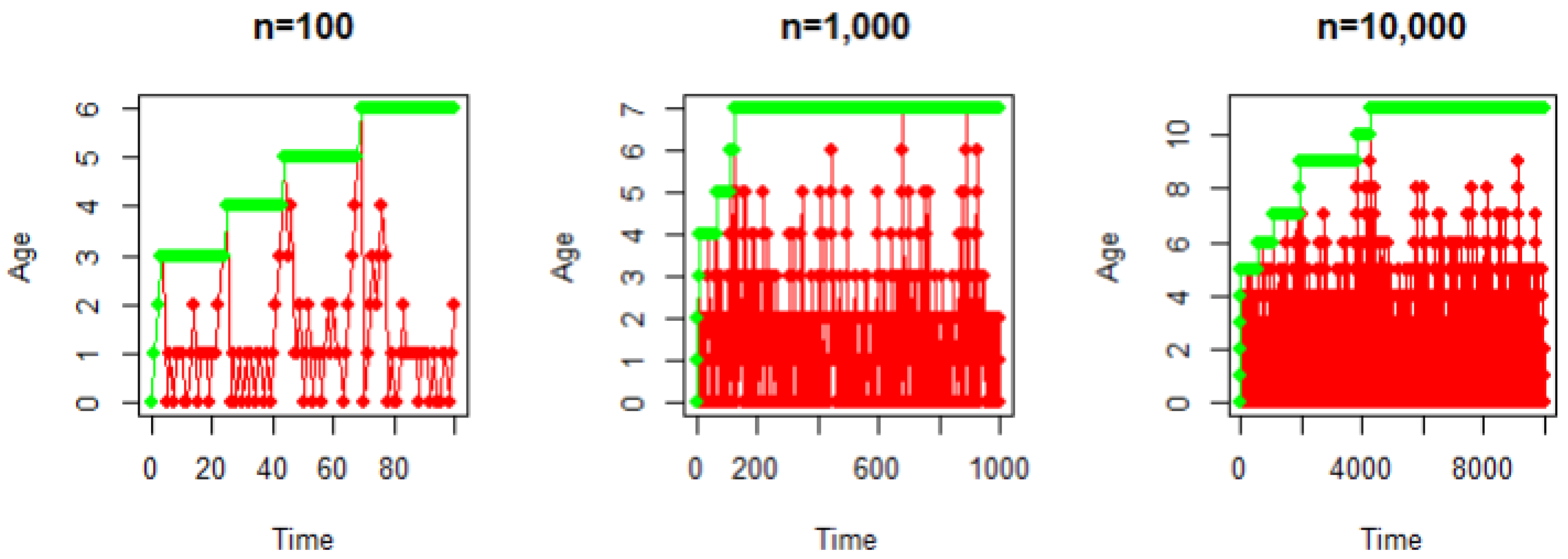
Figure 1. Simulation of walks X n (red) and H n (green).
Symmetry 16 01222 g001
Figure 2. Simulation of walks X n (red) and H n (green) when p 1 = 1 / 15 , p 2 = 2 / 15 , p 3 = 3 / 15 , p 4 = 4 / 15 and p 5 = 5 / 15 .
Symmetry 16 01222 g002
Disclaimer/Publisher’s Note: The statements, opinions and data contained in all publications are solely those of the individual author(s) and contributor(s) and not of MDPI and/or the editor(s). MDPI and/or the editor(s) disclaim responsibility for any injury to people or property resulting from any ideas, methods, instructions or products referred to in the content.