Article

Predictor Laplace Fractional Power Series Method for Finding Multiple Solutions of Fractional Boundary Value Problems

by
Abedel-Karrem Alomari
1,*,
Wael Mahmoud Mohammad Salameh
2,
Mohammad Alaroud
3,* and
Nedal Tahat
4
1
Department of Mathematics, Faculty of Science, Yarmouk University, Irbid 21163, Jordan
2
Faculty of Information Technology, Abu Dhabi University, Abu Dhabi P.O. Box 59911, United Arab Emirates
3
Department of Mathematics, Faculty of Arts and Science, Amman Arab University, Amman 11953, Jordan
4
Department of Mathematics, Faculty of Science, The Hashemite University, Zarqa 13133, Jordan
*
Authors to whom correspondence should be addressed.
Symmetry 2024, 16(9), 1152; https://doi.org/10.3390/sym16091152
Submission received: 6 June 2024 / Revised: 24 August 2024 / Accepted: 28 August 2024 / Published: 4 September 2024
(This article belongs to the Section Mathematics)

Abstract

:
This research focuses on finding multiple solutions (MSs) to nonlinear fractional boundary value problems (BVPs) through a new development, namely the predictor Laplace fractional power series method. This method predicts the missing initial values by applying boundary or force conditions. This research provides a set of theorems necessary for deriving the recurrence relations to find the series terms. Several examples demonstrate the efficacy, convergence, and accuracy of the algorithm. Under Caputo’s definition of the fractional derivative with symmetric order, the obtained results are visualized numerically and graphically. The behavior of the generated solutions indicates that altering the fractional derivative parameters within their domain symmetrically changes these solutions, ultimately aligning them with the standard derivative. The results are compared with the homotopy analysis method and are presented in various figures and tables.

1. Introduction

Recently, the topic of fractional-order differential equations (FODEs) has been recognized as a valuable, poignant, and qualitative instrument utilized in the formulation of complicated dynamical systems with ambiguous behavior. It includes numerous applications in mathematical physics, bio-mathematics, heat transfer engineering, quantum mechanics, nonlinear optics, fluid dynamics, electrical circuits, etc. In contrast, many studies have shown that fractional-order derivatives (FODs) can accurately interpret the memory and hereditary characteristics of various real-world phenomena [1,2,3,4,5].
In the literature, seeking exact and accurate approximate solutions to nonlinear FODEs is challenging for many scholars. It is a vital topic with theoretical and practical applications for various complicated natural phenomena involving local and non-local operators in different fields, including physics, chemistry, biology, finance, and engineering. Over the last few decades, numerous scholars have designed and developed efficient numerical and approximate methods to solve a wide range of linear and nonlinear FODEs, including but not limited to the variational iteration method (VIM), Laplace decomposition method (LTM) [6,7], Adomian decomposition method (ADM) [8], homotopy analysis method (HAM) [9], homotopy perturbation transform method (HPTM) [10], Yang transform decomposition method (YTDM) [11], and fractional power series method (FPSM) [12,13,14,15].
Due to the traditional power series (PS) approach becoming increasingly common, it has been more extensively utilized to treat fractional models when the classical-order derivative was updated to a FOD. The FPSM is a numerical and approximation scheme that has played a crucial role in solving intricate fractional models as well as in the simulation, analysis, and prediction of natural phenomena across various scientific disciplines. Its systematic scheme is based on determining the expansion series approximate solution to a wide range of FODEs by deriving the residual equation after substituting the suggested PS expansion into the target FODE and then equating the coefficients on both sides of the residual equation to detect the unknown parameters of the suggested PS approximate solution. To overcome this limitation, this study aims to improve the applicability and efficiency of the FPSM by combining it with the Laplace transform (LT) operator. The Laplace FPSM was initially presented and proven to obtain exact and approximate solutions of neutral pantograph equations of fractional order [16]. The proposed approach uses the LT to handle the difficulty of the nonlinear terms in the studied model, following the methodology of the FPSM in Laplace space. This combination offers advantages by reducing the computational efforts needed to find approximate solutions in the form of a fractional PS using the limit concept, unlike the FPSM, which utilizes an FOD in determining the unknown parameter at each stage of seeking a PS solution expansion.
In scientific studies, the Laplace FPSM is straightforward and has been successfully used to analyze and extract explicit and approximate series solutions for several types of fractional models, such as the fractional three-dimensional Helmholtz model [17], the time-fractional Korteveg–de Vries model [18], nonlinear fractional wave-like differential equations with variable coefficients [19], the Caudrey–Dodd–Gibbon model [20], the fractional Volterra integro-differential model [21], and the nonlinear time-fractional generalized biology population model [22].
Dual or multiple solution phenomena appear in several applications in physics and engineering, such as in fluid problems [23,24,25]. Finding multiple solutions to boundary value problems has been addressed by several methods, such as the homotopy analysis method (HAM) [26,27]. Xu and Liao found a dual solution for boundary layer flow over an upstream-moving plate using the HAM [28].
This paper refers to the new FPSM advancement as ’the predictor Laplace FPSM’. This study aims to employ the predictor Laplace FPSM in the sense of the Caputo FOD to extract multiple solutions (MSs) of a certain class of nonlinear FODEs with suitable boundary conditions. The algorithm is based on assuming some auxiliary initial conditions, applying the LFPSM, and then predicting those initial conditions by implementing the boundary or force conditions. The new algorithm does not require the selection of convergent control parameters, auxiliary linear operators, or initial guesses, as required in the HAM. Via this simple algorithm, a strongly nonlinear problem can be converted into a simple recurrence formula, the sum of which will converge to the exact solution. So, this paper addresses the question: How can the LFPSM generate multiple solutions for FDEs?

2. Preliminary and Notations

This section presents a summary of the main definitions and properties of the Caputo fractional derivative and Laplace transform, which are given in [19,22]. The α order of the Caputo fractional derivative is defined as
( D α f ) ( t ) = 1 Γ ( n α ) 0 t ( t x ) n α 1 f ( n ) ( x ) d x ,
where n 1 < α n , n N , provided the integration exists. Its Laplace transform is given by
L D α y ( t ) = s α Y ( s ) k = 0 n 1 s α k 1 y ( k ) ( 0 ) , α ( n 1 , n ] ,
where y ( t ) is a piecewise continuous function on [ 0 , ) and L [ y ( t ) ] = Y ( s ) for t [ 0 , ) . If L [ x ( t ) ] = X ( s ) , we have the following properties:
  • L [ a x ( t ) + b y ( t ) ] = a X ( s ) + b Y ( s ) .
  • L 1 [ a X ( s ) + b Y ( s ) ] = a x ( t ) + b y ( t ) .
  • lim s [ s Y ( s ) ] = y ( 0 ) .
  • L D k α y ( t ) = s k α Y ( s ) j = 0 k 1 s ( k j ) α 1 ( D j α y ) ( 0 ) , for α ( 0 , 1 ] .
Assuming that ( D n α f ) ( 0 ) exists for n = 1 , 2 , , then F ( s ) = L { f ( t ) } can be written in the following series expansion:
F ( s ) = n = 0 d n s n α + 1 , s > 0 , α ( 0 , 1 ] ,
where d n = ( D n α f ) ( 0 ) . Moreover, the remainder term of the above series using m terms is R m ( s ) = μ L [ D t ( m + 1 ) α f ( t ) ] ( μ ) s 1 + ( m + 1 ) α , and if μ L [ D t ( m + 1 ) α f ( t ) ] ( μ ) , where 0 < α 1 , then
R m ( s ) s 1 + ( m + 1 ) α , 0 < s μ .

3. Predictor Laplace FPSM

Consider the following BVP:
D α y ( t ) = N [ t , y ( t ) ] , n 1 < α n ,
where N ( t , y ) is the nonlinear term, subject to the conditions
B ( y , d y d t , d 2 y d y 2 , ) = 0 .
The predictor Laplace fractional power series method (FPSM) algorithm is detailed through the following steps:
  • Assume the initial conditions y ( i ) ( 0 ) = A i .
  • Apply the LT to Equation (4) to obtain
    Y ( s ) i = 0 n 1 y ( i ) ( 0 ) s i + 1 = 1 s α L [ N ( t , y ) ] .
  • Assume that Y ( s ) and the LT of the nonlinear term can be formulated as
    Y ( s ) = i = 0 J ( c i s q i + 1 ) ,
    L [ N ( t , y ] = i = s 1 s 2 ( w i s q i + 1 ) ,
    where the parameter q is in the form 1 / n ; n N such that α = n 1 + α 1 q ; α 1 N , and s 1 and J s 2 are fixed positive integers depending on the nonlinear terms.
  • Set the c i for i = 0 , 1 , 2 , ( n 1 ) / q + α 1 as c 0 = A 0 = y ( 0 ) , c 1 / q = A 1 = y ( 0 ) , c 2 / q = A 2 = y ( 0 ) , c ( n 1 ) / q = y ( n 1 ) ( 0 ) = A n 1 , and c i = 0 for the other values.
  • Substitute Equations (7) and (8) into the residual error to obtain
    R J = i = 0 J ( c i s q i + 1 ) ( w i s q [ ( n 1 ) / q + α 1 + i ] + 1 ) .
  • Multiply (9) by s j q + 1 and take the limit lim s s j q + 1 R j = 0 to obtain
    lim s s j q + 1 R j = lim s i = 0 j ( c i s q ( i j ) ) ( w i s q [ ( n 1 ) / q + α 1 + i j ] ) = 0 .
    This gives c i = w i ( n 1 ) / q α 1 for i > ( n 1 ) / q + α 1 .
  • Apply the inverse Laplace transform to Equation (8); the N-th order of the approximate solution becomes
    y ( t , A n 1 ) = i = 0 N c i t q i Γ ( q i + 1 ) .
    where A n 1 is the vector { A 0 , A 1 , A 2 , A n 1 } .
  • Substitute the solution y ( t , A n 1 ) into the conditions in Equation (5) to generate n-nonlinear algebraic equations.
  • Solve the equations generated in Step 8 using an accurate method such as the Newton–Raphson method or the new optimal numerical root-solver [29] to determine all solutions for the unknown A i .
  • Substitute the solutions for A i from Step 9 into y ( t , A n 1 ) to obtain the complete solution to Equation (4).
Typically, it is challenging to express the Laplace transform of nonlinear operators as shown in Equation (8), particularly for functions such as trigonometric, exponential, and root functions, for example, tan ( y ) , e y 2 and y 2 + 1 . These functions may be approximated using the Taylor series and then applied in the form of L [ y n ] .
In the following, we introduce the expansion for some nonlinear operators L [ N ( t , y ) ] that are needed in this paper.
Theorem 1.
The LT of the nonlinear operator d y d t 2 using the Laplace PS is
L d [ L 1 Y ( s ) ] d t = n = 2 2 j q 2 s 1 n q Γ ( n q 1 ) i = max ( 1 , n j ) min ( j , n ) c i c n i Γ ( q i ) Γ ( q ( n i ) ) .
Proof. 
d [ L 1 Y ( s ) ] d t = d [ L 1 i = 0 j c i s q i + 1 ] d t = d d t i = 0 J c i t q i Γ ( q i + 1 ) = i = 1 j c i t q ( i 1 / q ) Γ ( q i ) .
The nonlinear [ y ( t ) ] 2 can be written as
[ y ( t ) ] 2 = i = 1 j c i t q ( i 1 / q ) Γ ( q i ) × i = 1 j c i t q ( i 1 / q ) Γ ( q i ) ,
= n = 2 2 j q 2 t q n 2 q i = max ( 1 , n j ) min ( j , n ) c i c n i Γ ( i q ) Γ ( ( n i ) q ) .
Apply LT to obtain the result in Equation (12). □
Theorem 2.
The LT of the nonlinear operator 1 y 3 ( t ) using the Laplace PS is
L 1 [ L 1 Y ( s ) ] 3 = i = 0 3 J + N b i s q i + 1 ,
where
b 0 = 1 c 0 3 ,
b i = i 1 = 1 i b i i 1 b 0 3 i 2 = 0 i 1 c i 1 i 2 Γ ( q ( i 1 i 2 ) + 1 ) i 3 = 0 i 2 c i 3 c i 2 i 3 Γ ( q i 3 + 1 ) Γ ( q ( i 2 i 3 ) + 1 ) .
Proof. 
Assume
1 [ L 1 Y ( s ) ] 3 = 1 i = 0 J c i t q i Γ ( q i + 1 ) 3 = i = 0 V b i t q i .
For J > 0 , we have
1 = i = 0 J c i t q i Γ ( q i + 1 ) 3 × i = 0 V b i t q i , = i = 0 3 J + V t q i i 1 = max ( 0 , i J ) min ( i , 3 J ) b i i 1 i 2 = max ( 0 , i 1 J ) min ( i , 2 J ) c i 1 i 2 Γ ( q ( i 1 i 2 ) + 1 ) i 3 = max ( 0 , i 2 J ) min ( i , J ) c i 3 c i 2 i 3 Γ ( q i 3 + 1 ) Γ ( q ( i 2 i 3 ) + 1 ) , = b i c 0 3 + i = 1 3 J + V t q i i 1 = max ( 1 , i J ) min ( i , 3 J ) b i i 1 i 2 = max ( 0 , i 1 J ) min ( i , 2 J ) c i 1 i 2 Γ ( q ( i 1 i 2 ) + 1 ) i 3 = max ( 0 , i 2 J ) min ( i , J ) c i 3 c i 2 i 3 Γ ( q i 3 + 1 ) Γ ( q ( i 2 i 3 ) + 1 ) .
By equating the coefficients of the same order of t q i , we have
b 0 = 1 c 0 3 , b i = i 1 = 1 i b ( i i 1 ) b 0 3 i 2 = 0 i 1 c ( i 1 i 2 ) Γ ( q ( i 1 i 2 ) + 1 ) i 3 = 0 i 2 c ( i 3 ) c ( i 2 i 3 ) Γ ( q i 3 + 1 ) Γ ( q ( i 2 i 3 ) + 1 ) .
Now, apply the LT to obtain Equation (16). □

4. Applications

In this section, two examples are provided to validate the proposed algorithm. The first example involves the one-dimensional steady-state heat conduction equation in dimensionless form, which represents the temperature distribution of a straight rectangular fin with a power-law temperature-dependent surface heat flux [8]. The second example involves the governing balance equations for the velocity field of mixed convection flows, combining forced and free flows in the fully developed vertical channel region with isothermal walls maintained at the same temperature [30]. The following models are the counterparts of these examples, utilizing the Caputo fractional derivative.
Example 1.
Consider the following nonlinear FODE:
D α y ( t ) = 4 25 y 3 , 1 < α 2 ,
subject to the boundary conditions y ( 0 ) = 0 , y ( 1 ) = 1 .
To start with the predictor Laplace FPSM, we begin with the initial conditions y ( 0 ) = A , y ( 0 ) = 0 , and then we apply the LT
Y ( s ) = y ( 0 ) s + 1 s α L [ 1 ( L 1 Y ( s ) ) 3 ] .
With the help of the Theorem 2, the series expansion of the problem is
i = 0 J c i s q i + 1 = A s + 4 25 1 s 1 / q + α 1 i = 0 J b i s q i + 1 .
Using some simplifications, multiply the residual by s n q + 1 and take the limit to obtain
lim s s n q + 1 R J = lim s i = 0 J c i s q ( i n ) A s n q 4 25 1 s 1 / q + α 1 i = 0 J b i s q ( i + 1 / q + a 1 n ) = 0 .
By shifting the index, we can obtain the recurrence relation
c n = 4 25 b n 1 / q α 1 , n 1 / q + α 1 ,
and c 0 = A , c i = 0 for i = 1 , 2 , 1 / q + α 1 1 .
For α = 1.9 , we can choose q = 1 / 10 and α 1 = 9 to obtain the series
y ( t ) i = 0 100 c i t 0.1 i Γ ( 0.1 i + 1 ) = 0.00235611 A 5 t 19 / 5 + 0.0875582 t 19 / 10 A 3 + A .
Applying the boundary condition y ( 1 ) = 1 , the values of A are { 0.605212 , 0.866628 } . We test the convergence of the method in the next section.
Example 2.
Consider the following fractional problem:
D α y ( t ) = σ 16 d y ( t ) d t 2 , 3 < α 4 .
It is subject to the conditions
y ( 0 ) = y ( 0 ) = y ( 1 ) = 0 , 0 1 y ( t ) d t = 1 .
The algorithm suggests the following initial conditions
y ( 0 ) = A 0 , y ( 0 ) = y ( 0 ) = 0 , y ( 0 ) = A 2 .
Take the LT for Equation (22), apply Theorem 1, and then take the limit of the s n q + 1 R J as s as
lim s s n q + 1 R J = lim s i = 0 J c i s q ( i n ) A 0 s n q A 2 s q ( n + 2 / q ) s n q + 1 s 3 + q α 1 × σ 16 i = 2 2 j q 2 Γ ( i q 1 ) s i q 1 i 1 = max ( 1 , i 1 j ) min ( j , i ) c i 1 c i i 1 Γ ( q i 1 ) Γ ( q ( i i 1 ) ) , = lim s i = 0 J c i s q ( i n ) A 0 s n q A 2 s q ( n + 2 / q ) σ 16 i = 2 2 j q 2 Γ ( i q 1 ) s q ( i + α 1 n + 1 / q ) ) i 1 = max ( 1 , i 1 j ) min ( j , i ) c i 1 c i i 1 Γ ( q i 1 ) Γ ( q ( i i 1 ) ) = 0 .
By shifting the index and equating the same coefficients of s q i , the following recurrence relation is obtained
c n = σ 16 q 2 Γ q n α 1 1 q 1 i = 1 α 1 + n 1 q i c i α 1 i + n 1 q c α 1 i + n 1 q Γ ( i q + 1 ) Γ q i + n α 1 1 q + 1 ,
for n 3 / q + 1 , and c i = 0 , i = 1 , 2 , 3 / q , i 2 / q , c 0 = A 0 , c 2 / q = A 2 . If α , q are fixed, the solution will depend on A 0 and A 2 , which can be obtained by applying the conditions y ( 1 ) = 0 , 0 1 y ( t ) d t = 1 .
For instance, if α = 3.9 , we can choose q = 1 / 10 , α 1 = 9 . The approximate solution is
y ( t ) i = 0 300 c i t 0.1 t Γ ( 0.1 i + 1 ) = A 0 9.30283 × 10 18 A 2 8 t 293 / 10 + 2.80286 × 10 15 A 2 7 t 127 / 5 8.30589 × 10 13 A 2 6 t 43 / 2 + 2.3739 × 10 10 A 2 5 t 88 / 5 6.71836 × 10 8 A 2 4 t 137 / 10 + 0.0000162333 A 2 3 t 49 / 5 0.00418414 A 2 2 t 59 / 10 + 0.5 A 2 t 2 .
By the condition y ( 1 ) = 0 , the value of A 0 is i = 1 300 c i Γ ( 0.1 i + 1 ) . Additionally, the integration condition 0 1 y ( t ) d t = 1 can be solved to obtain A 2 = { 2.90813 , 145.878 } , which are two solutions.
This study examines the convergence of the algorithm and the solution behaviors for different values of α . Table 1 presents the values of A for different fractional derivatives and the N-th order of approximation for Example 1. It is observed that the values of A converge as the order increases. Specifically, for α = 1.9 , the values of A are { 0.4507 , 0.8801 } using the homotopy analysis method (HAM) [9]. Experimentally, the solution continues to converge as the values of α decrease from 2 to 1.68, beyond which no solutions exist for the equation y ( 1 ) = 1 . The effect of varying α on the solution is illustrated in Figure 1.
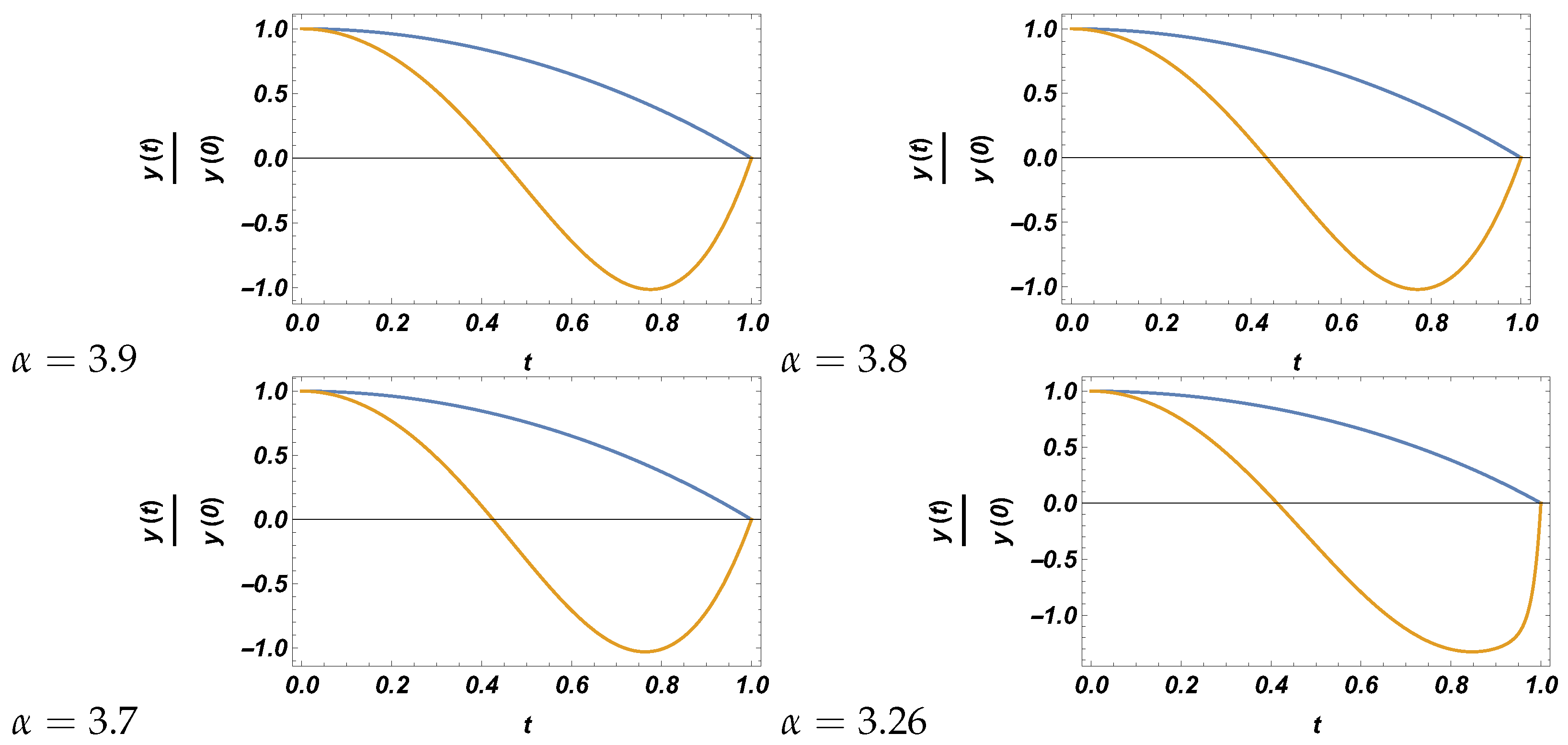
For Example 2, fixing σ = 20 and σ = 20 , the values of A 2 for various α and different N-th order approximations are provided in Table 2 and Table 3, respectively. These tables demonstrate that the solution converges to fixed values for A 2 . Notably, the values of A 2 using the HAM at σ = 20 were found to be { 2.908 , 148.367 } for α = 3.9 , which aligns closely with our findings. The experimental results indicate that the problem has multiple solutions for 3.26 α 4 . The ratio y ( t ) y ( 0 ) using the 700th order of the approximate solution for different α values is depicted in Figure 2.
Lastly, Table 4 and Table 5 present the solutions for Example 2 at σ = 20 and σ = 20 , respectively. These tables provide the numerical values of the dual solution for different α at several values of t using the 700th order of approximation. The first rows of these tables at t = 0 represent the values of A 0 , while the values in the last row at t = 1 represent the numerical approximations of y ( 1 ) , which are very close to zero.

5. Conclusions and Future Work

Comprehension of the existence and characteristics of MSs is crucial for gaining insights into the behavior of sophisticated phenomena described by FODEs. In this study, a new and superior algorithm has been designed to investigate the MSs for nonlinear fractional BVPs in the context of Caputo FODs. The proposed algorithm has successfully generated an approximate analytic solution with simple recurrence formulas and can be applied directly without any linearization or discretization of the domain. Unlike other approximations, this method does not require the selection of convergent parameters. The findings reveal that the proposed algorithm is an effective and simple methodology method for finding MSs. Therefore, this study recommends that the predictor LFPSM be applied to solve such complex problems using different definitions of fractional derivatives, such as Hadamard and Sonin–Letnikov, or to some fluid models as given in references [23,24,25], which may lead to different solution behaviors.

Author Contributions

Conceptualization, A.-K.A. and M.A.; methodology, A.-K.A.; software, N.T.; validation, W.M.M.S. and M.A.; formal analysis, A.-K.A.; investigation, N.T.; resources, W.M.M.S.; data curation, N.T.; writing—original draft preparation, A.-K.A.; writing—review and editing, M.A.; visualization, W.M.M.S.; supervision, N.T.; project administration, A.-K.A.; funding acquisition, W.M.M.S. All authors have read and agreed to the published version of the manuscript.

Funding

This research received no external funding.

Data Availability Statement

Data are contained within the article.

Conflicts of Interest

The authors declare no conflicts of interest.

References

  1. Veeresha, P.; Prakasha, D.G.; Kumar, S. A fractional model for propagation of classical optical solitons by using nonsingular derivative. Math. Methods Appl. Sci. 2024, 45, 10609–10623. [Google Scholar] [CrossRef]
  2. Kumar, S. A new fractional modeling arising in engineering sciences and its analytical approximate solution. Alex. Eng. J. 2013, 52, 813–819. [Google Scholar] [CrossRef]
  3. Partohaghighi, M.; Akgül, A.; Guran, L.; Bota, M.F. Novel mathematical modelling of platelet-poor plasma arising in a blood coagulation system with the fractional Caputo–Fabrizio derivative. Symmetry 2022, 14, 1128. [Google Scholar] [CrossRef]
  4. Kumar, P.; Baleanu, D.; Erturk, V.S.; Inc, M.; Govindaraj, V. A delayed plant disease model with Caputo fractional derivatives. Adv. Contin. Discret. Models 2022, 1, 11. [Google Scholar] [CrossRef]
  5. Baleanu, D.; Qureshi, S.; Yusuf, A.; Soomro, A.; Osman, M.S. Bi-modal COVID-19 transmission with Caputo fractional derivative using statistical epidemic cases. Partial. Differ. Equations Appl. Math. 2024, 10, 100732. [Google Scholar] [CrossRef]
  6. Khuri, S.A. A Laplace decomposition algorithm applied to a class of nonlinear differential equations. J. Appl. Math. 2002, 1, 141–155. [Google Scholar] [CrossRef]
  7. Ray, S.S. Analytical solution for the space fractional diffusion equation by two-step Adomian decomposition method. Commun. Nonlinear Sci. Numer. Simul. 2009, 14, 1295–1306. [Google Scholar]
  8. Chang, M.H. A decomposition solution for fins with temperature dependent surface heat flux. Int. J. Heat Mass Transf. 2005, 48, 1819–1824. [Google Scholar] [CrossRef]
  9. Alomari, A.K.; Awawdeh, F.; Tahat, N.; Ahmad, F.B.; Shatanawi, W. Multiple solutions for fractional differential equations: Analytic approach. Appl. Math. Comput. 2013, 219, 8893–8903. [Google Scholar] [CrossRef]
  10. Khan, Y.; Wu, Q. Homotopy perturbation transform method for nonlinear equations using He’s polynomials. Comput. Math. Appl. 2011, 61, 1963–1967. [Google Scholar] [CrossRef]
  11. Naeem, M.; Yasmin, H.; Shah, R.; Shah, N.A.; Chung, J.D. A comparative study of fractional partial differential equations with the help of yang transform. Symmetry 2023, 15, 146. [Google Scholar] [CrossRef]
  12. Khader, M.M.; Babatin, M.M. On approximate solutions for fractional logistic differential equation. Math. Probl. Eng. 2013, 2013, 391901. [Google Scholar] [CrossRef]
  13. Zidan, A.M.; Khan, A.; Shah, R.; Alaoui, M.K.; Weera, W. Evaluation of time-fractional Fisher’s equations with the help of analytical methods. AIMS Math. 2022, 7, 18746–18766. [Google Scholar] [CrossRef]
  14. Aljarrah, H.; Alaroud, M.; Ishak, A.; Darus, M. Adaptation of residual-error series algorithm to handle fractional system of partial differential equations. Mathematics 2021, 9, 2868. [Google Scholar] [CrossRef]
  15. Ismail, G.M.; Abdl-Rahim, H.R.; Ahmad, H.; Chu, Y.M. Fractional residual power series method for the analytical and approximate studies of fractional physical phenomena. Open Phys. 2020, 18, 799–805. [Google Scholar] [CrossRef]
  16. Eriqat, T.; El-Ajou, A.; Moa’ath, N.O.; Al-Zhour, Z.; Momani, S. A new attractive analytic approach for solutions of linear and nonlinear neutral fractional pantograph equations. Chaos Solitons Fractals 2020, 138, 109957. [Google Scholar] [CrossRef]
  17. Albalawi, W.; Shah, R.; Nonlaopon, K.; El-Sherif, L.S.; El-Tantawy, S.A. Laplace Residual Power Series Method for Solving Three-Dimensional Fractional Helmholtz Equations. Symmetry 2023, 15, 194. [Google Scholar] [CrossRef]
  18. Yadav, S.; Vats, R.K.; Rao, A. Constructing the fractional series solutions for time-fractional K-dV equation using Laplace residual power series technique. Opt. Quantum Electron. 2024, 56, 721. [Google Scholar] [CrossRef]
  19. Alaroud, M.; Aljarrah, H.; Alomari, A.K.; Ishak, A.; Darus, M. Explicit and approximate series solutions for nonlinear fractional wave-like differential equations with variable coefficients. Partial. Differ. Equations Appl. Math. 2024, 10, 100680. [Google Scholar] [CrossRef]
  20. Abdelhafeez, S.A.; Arafa, A.A.; Zahran, Y.H.; Osman, I.S.; Ramadan, M. Adapting Laplace residual power series approach to the Caudrey Dodd Gibbon equation. Sci. Rep. 2024, 14, 9772. [Google Scholar] [CrossRef]
  21. Alomari, A.K.; Alaroud, M.; Tahat, N.; Almalki, A. Extended Laplace power series method for solving nonlinear Caputo fractional Volterra integro-differential equations. Symmetry 2023, 15, 1296. [Google Scholar] [CrossRef]
  22. Alaroud, M.; Alomari, A.K.; Tahat, N.; Ishak, A. Analytical Computational Scheme for Multivariate Nonlinear Time-Fractional Generalized Biological Population Model. Fractal Fract. 2023, 7, 176. [Google Scholar] [CrossRef]
  23. Yahaya, R.I.; Md Arifin, N.; Pop, I.; Md Ali, F.; Mohamed Isa, S.S.P. Dual solutions for MHD hybrid nanofluid stagnation point flow due to a radially shrinking disk with convective boundary condition. Int. J. Numer. Methods Heat Fluid Flow 2023, 33, 456–476. [Google Scholar] [CrossRef]
  24. Khan, M.; Ahmad, L.; Yasir, M.; Ahmed, J. Numerical analysis in thermally radiative stagnation point flow of cross nanofluid due to shrinking surface: Dual solutions. Appl. Nanosci. 2023, 13, 573–584. [Google Scholar] [CrossRef]
  25. Saleem, M.; Hussain, M. Dual solutions of Williamson-Casson fluid over a heated exponentially shrinking surface with stability analysis: A novel Catteneo-Christov heat flux model combination. Numer. Heat Transf. Part A Appl. 2024, 85, 114–136. [Google Scholar] [CrossRef]
  26. Abbasbandy, S.; Magyari, E.; Shivanian, E. The homotopy analysis method for multiple solutions of nonlinear boundary value problems. Commun. Nonlinear Sci. Numer. Simul. 2009, 14, 3530–3536. [Google Scholar] [CrossRef]
  27. Abbasbandy, S.; Shivanian, E. Prediction of multiplicity of solutions of nonlinear boundary value problems: Novel application of homotopy analysis method. Commun. Nonlinear Sci. Numer. Simul. 2010, 15, 3830–3846. [Google Scholar] [CrossRef]
  28. Xu, H.; Liao, S.J. Dual solutions of boundary layer flow over an upstream moving plate. Commun. Nonlinear Sci. Numer. Simul. 2008, 13, 350–358. [Google Scholar] [CrossRef]
  29. Qureshi, S.; Chicharro, F.I.; Argyros, I.K.; Soomro, A.; Alahmadi, J.; Hincal, E. A New Optimal Numerical Root-Solver for Solving Systems of Nonlinear Equations Using Local, Semi-Local, and Stability Analysis. Axioms 2024, 13, 341. [Google Scholar] [CrossRef]
  30. Abbasbandy, S.; Shivanian, E. Predictor homotopy analysis method and its application to some nonlinear problems. Commun. Nonlinear Sci. Numer. Simul. 2011, 16, 2456–2468. [Google Scholar] [CrossRef]
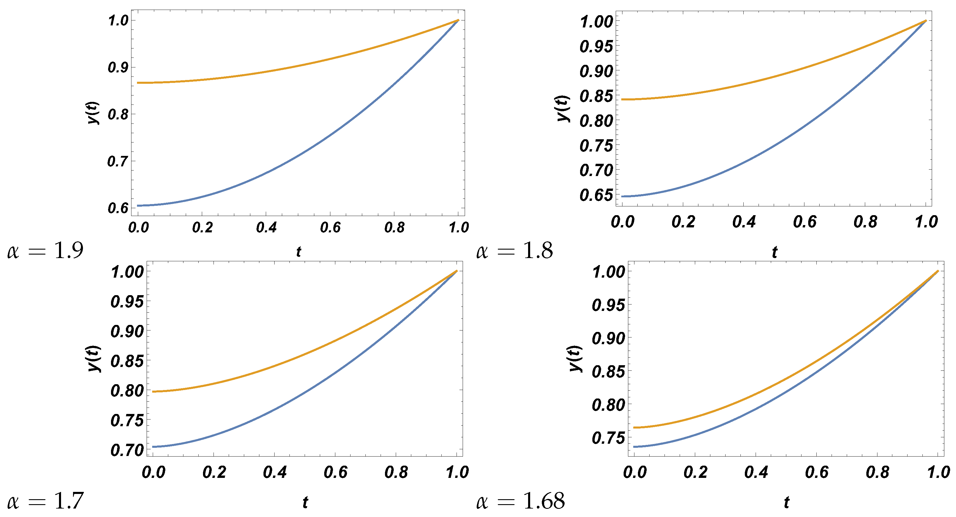
Figure 1. The solutions of Example 1 using the 70th order of approximation for α = 1.9 , 1.8 , 1.7 , 1.68 . The first and the second solution are represent in the orange and blue curves respectively.
Symmetry 16 01152 g001
Figure 2. The solutions of Example 2 using the 700th order of approximation for α = 3.9 , 3.8 , 3.7 , 3.26 . The first and the second solution are represent in the blue and orange curves respectively.
Symmetry 16 01152 g002
Table 1. The values of A for different α and n-th orders for Example 1.
n α = 1.9 α = 1.8 α = 1.7
400.60521209620.86662804970.64542995870.84098461220.70406908990.7968988326
500.60521209620.86662804970.64542995870.84098461220.70406908990.7968988326
600.60520652650.86663399060.64541233010.84100564560.70397995710.7970001618
700.60520652650.86663399060.64541233010.84100564560.70397956810.7970000599
800.60520649870.86663396320.64541223630.84100557100.70397956810.7970000599
900.60520649870.86663396320.64541223640.84100557080.70397956960.7970000577
1000.60520649870.86663396320.64541223640.84100557080.70397956960.7970000577
Table 2. The values of A 2 for different α and n-th orders using σ = 20 for Example 2.
n α = 3.9 α = 3.8 α = 3.7
300−2.908126478145.8780662−2.890668959125.3769389−2.870259296106.3892558
400−2.908126478147.7398896−2.890668959131.8532334−2.870259296113.2663820
500−2.908126478148.4348950−2.890668959130.8731202−2.870259296118.8103639
600−2.908126478148.3813672−2.890668959130.4388597−2.870259296115.3101551
700−2.908126478148.3654474−2.890668959130.4794925−2.870259296115.9764097
800−2.908126478148.3669774−2.890668959130.4985713−2.870259296115.7959115
900−2.908126478148.3668728−2.890668959130.4956720−2.870259296115.8171922
1000−2.908126478148.3668434−2.890668959130.4959435−2.870259296115.8344660
Table 3. The values of A 2 for different α and n-th orders using σ = 20 for Example 2.
n α = 3.9 α = 3.8 α = 3.7
300−138.0711661−3.101976104−118.1546084−3.123617677−100.1782084−3.149851401
400−139.3947405−3.101976104−122.1853108−3.123617677−109.4983522−3.149851401
500−139.7981285−3.101976104−121.7141473−3.123617677−107.3604086−3.149851401
600−139.7714048−3.101976104−121.5374888−3.123617677−106.3390332−3.149851401
700−139.7646425−3.101976104−121.5522702−3.123617677−106.524706−3.149851401
800−139.7651863−3.101976104−121.5578166−3.123617677−106.4873698−3.149851401
900−139.7651539−3.101976104−121.5571362−3.123617677−106.4913908−3.149851401
1000−139.7651461−3.101976104−121.5571918−3.123617677−106.4937748−3.149851401
Table 4. The solutions y ( t ) of Example 2 with σ = 20 using the 700th order of approximation at several values of t.
t y ( t ) for α = 3.9 y ( t ) for α = 3.8 y ( t ) for α = 3.7
0.001.48985−13.71521.48802−11.62331.48590−9.89024
0.251.39896−9.104451.39768−7.572711.39619−6.30149
0.501.125743.345401.125933.219571.126163.11011
0.750.6654413.76430.66705311.79560.66891410.1577
1.003.04497 × 10 18 4.16334 × 10 16 9.49464 × 10 17 1.03251 × 10 14 −5.60716 × 10 17 1.66533 × 10 14
Table 5. The solutions y ( t ) of Example 2 with σ = 20 using the 700th order of approximation at several values of t.
t y ( t ) for α = 3.9 y ( t ) for α = 3.8 y ( t ) for α = 3.7
0.0015.29271.5112113.2051.5134511.47981.51614
0.2510.94791.414289.430371.415858.176211.41773
0.50−0.8570151.12413−0.7101991.12388−0.5827391.12356
0.75−11.25940.646121−9.317460.644145−7.713110.6418
1.008.88178 × 10 16 2.93434 × 10 16 −2.9976 × 10 15 1.78424 × 10 16 −5.9952 × 10 15 −1.09784 × 10 16
Disclaimer/Publisher’s Note: The statements, opinions and data contained in all publications are solely those of the individual author(s) and contributor(s) and not of MDPI and/or the editor(s). MDPI and/or the editor(s) disclaim responsibility for any injury to people or property resulting from any ideas, methods, instructions or products referred to in the content.