

Estimation of Marshall–Olkin Extended Generalized Extreme Value Distribution Parameters under Progressive Type-II Censoring by Using a Genetic Algorithm


Abstract
1. Introduction
2. Marshall–Olkin Extended Generalized Extreme Value under Linear Normalization Distribution and Cases of Type-II Progressive Censored Scheme Considered
2.1. Marshall–Olkin Extended Generalized Extreme Value under Linear Normalization Distribution
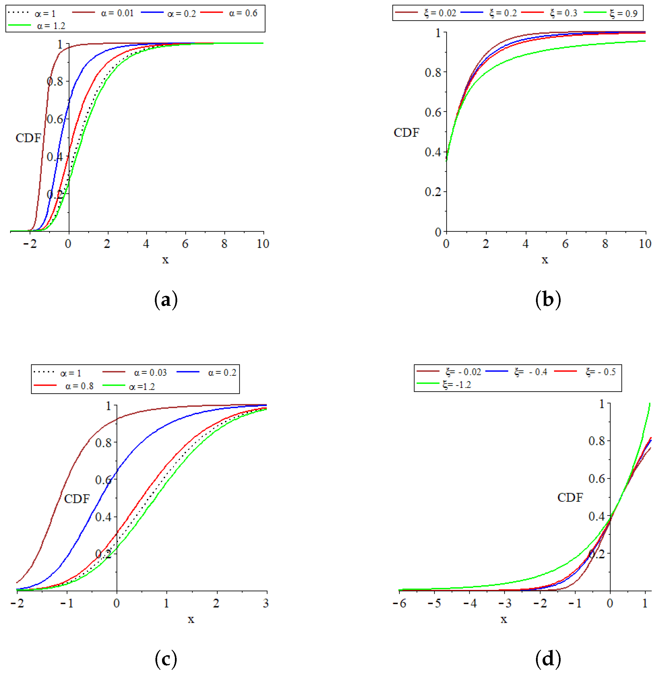
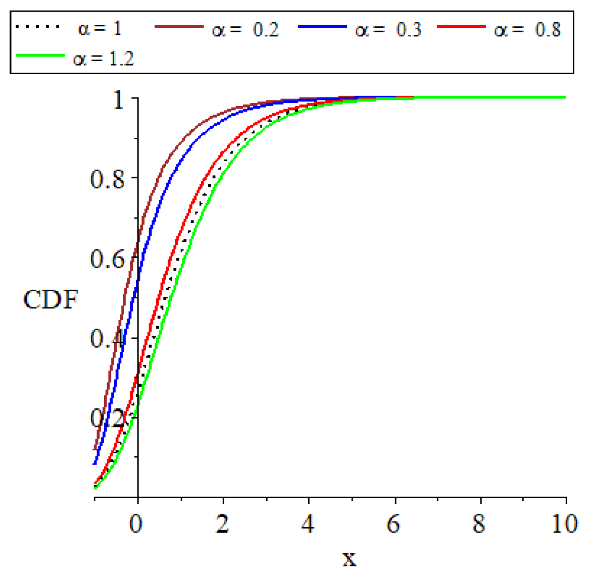
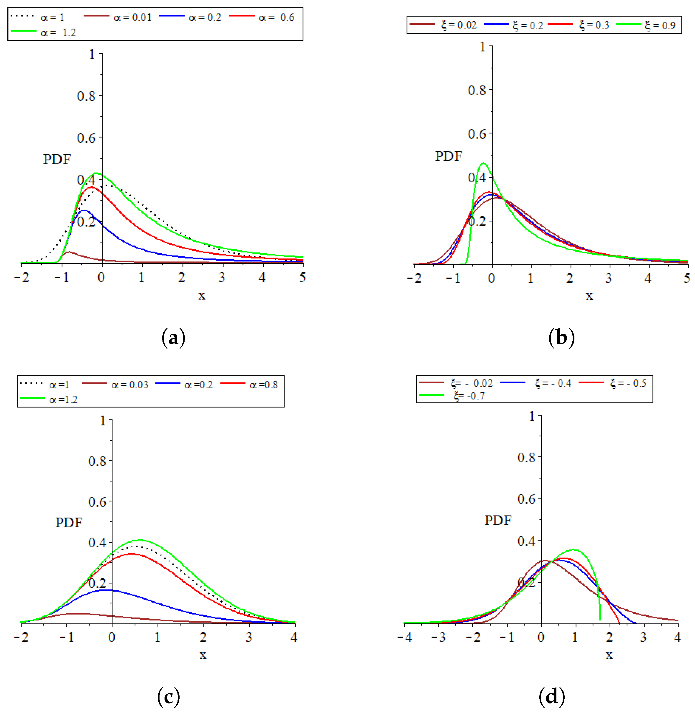
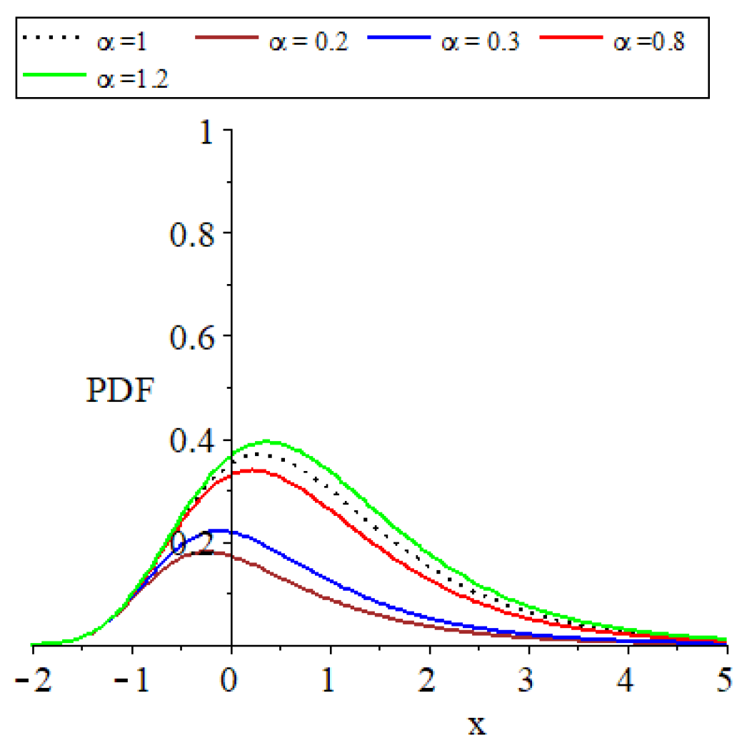
- 2:
- 3:
- 4:
- The provided plots effectively show the remarkable flexibility of the models introduced.
2.2. Cases of Type-II Progressive Censored Scheme Considered
- The first scenario: Fixed Removal Censoring Scheme
- The second scenario: Removals With Discrete Uniform Distribution
- The third scenario: Removals With Binomial Distribution
3. Maximum Likelihood Estimation of Parameters and Observed Fisher Information
3.1. Maximum Likelihood Estimation of Parameters
- The first scenario:
- The second scenario:
- The third scenario:
3.2. Observed Fisher Information and Approximate Confidence Interval Concerning the Distribution of the Censoring Scheme
3.2.1. Observed Fisher Information Corresponding
3.2.2. The Asymptotic Confidence Interval
4. Bayesian Estimation
Lindley’s Approximation Method
5. Simulation
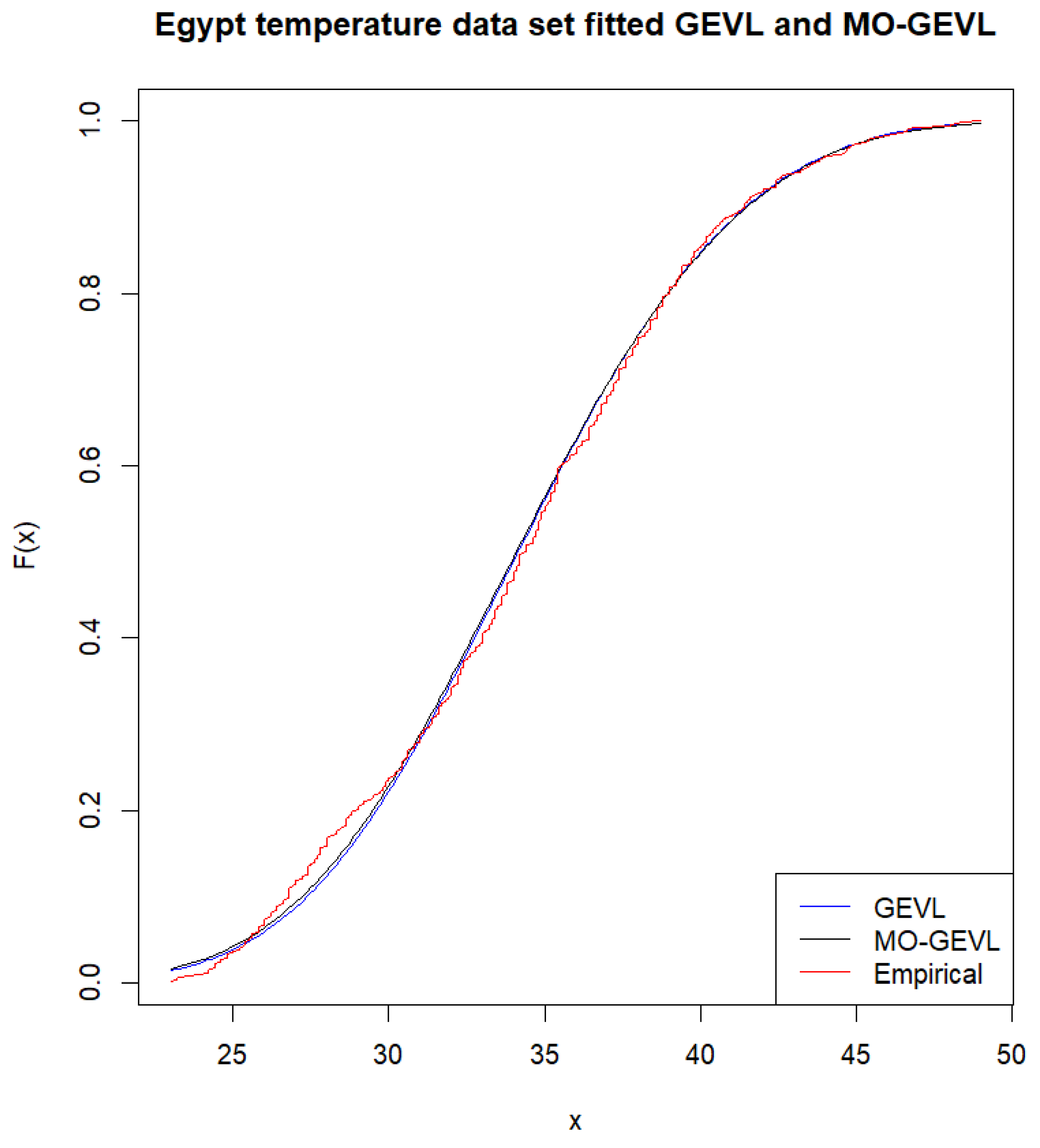
6. Real Data Example
7. Conclusions
Author Contributions
Funding
Data Availability Statement
Acknowledgments
Conflicts of Interest
References
- Gilli, M.; Këllezi, E. An application of extreme value theory for measuring financial risk. Comput. Econ. 2006, 27, 207–228. [Google Scholar] [CrossRef]
- Fisher, R.A.; Tippett, L.H.C. Limiting forms of the frequency distribution of the largest or smallest member of a sample. In Mathematical Proceedings of the Cambridge Philosophical Society; Cambridge University Press: Cambridge, UK, 1928; Volume 24, pp. 180–190. [Google Scholar]
- Bali, T.G. The generalized extreme value distribution. Econ. Lett. 2003, 79, 423–427. [Google Scholar] [CrossRef]
- Hosking, J.R.M.; Wallis, J.R.; Wood, E.F. Estimation of the generalized extreme-value distribution by the method of probability-weighted moments. Technometrics 1985, 27, 251–261. [Google Scholar] [CrossRef]
- Bertin, E.; Clusel, M. Generalized extreme value statistics and sum of correlated variables. J. Phys. A Math. Gen. 2006, 39, 7607. [Google Scholar] [CrossRef]
- Hu, X.; Fang, G.; Yang, J.; Zhao, L.; Ge, Y. Simplified models for uncertainty quantification of extreme events using Monte Carlo technique. Reliab. Eng. Syst. Saf. 2023, 230, 108935. [Google Scholar] [CrossRef]
- Ali, Y.; Haque, M.M.; Mannering, F. A Bayesian generalised extreme value model to estimate real-time pedestrian crash risks at signalised intersections using artificial intelligence-based video analytics. Anal. Methods Accid. Res. 2023, 38, 100264. [Google Scholar] [CrossRef]
- Lovell, C.C.; Harrison, I.; Harikane, Y.; Tacchella, S.; Wilkins, S.M. Extreme value statistics of the halo and stellar mass distributions at high redshift: Are JWST results in tension with ΛCDM? Mon. Not. R. Astron. Soc. 2023, 518, 2511–2520. [Google Scholar] [CrossRef]
- Marshall, A.W.; Olkin, I. A new method for adding a parameter to a family of distributions with application to the exponential and Weibull families. Biometrika 1997, 84, 641–652. [Google Scholar] [CrossRef]
- Jose, K. Marshall-Olkin family of distributions and their applications in reliability theory, time series modeling and stress-strength analysis. In Proceedings of the 58th World Statistical Congress, Dublin, Ireland, 21–26 August 2011; Volume 201, pp. 3918–3923. [Google Scholar]
- Obulezi, O.J.; Anabike, I.C.; Oyo, O.G.; Igbokwe, C.; Etaga, H. Marshall-Olkin Chris-Jerry distribution and its applications. Int. J. Innov. Sci. Res. Technol. 2023, 8, 522–533. [Google Scholar]
- Ozkan, E.; Golbasi Simsek, G. Generalized Marshall-Olkin exponentiated exponential distribution: Properties and applications. PLoS ONE 2023, 18, e0280349. [Google Scholar] [CrossRef]
- Niyoyunguruza, A.; Odongo, L.O.; Nyarige, E.; Habineza, A.; Muse, A.H. Marshall-Olkin Exponentiated Frechet Distribution. J. Data Anal. Inf. Process. 2023, 11, 262–292. [Google Scholar]
- Alsadat, N.; Nagarjuna, V.B.; Hassan, A.S.; Elgarhy, M.; Ahmad, H.; Almetwally, E.M. Marshall–Olkin Weibull–Burr XII distribution with application to physics data. AIP Adv. 2023, 13, 095325. [Google Scholar] [CrossRef]
- Phoong, S.Y.; Ismail, M.T. A comparison between Bayesian and maximum likelihood estimations in estimating finite mixture model for financial data. Sains Malays. 2015, 44, 1033–1039. [Google Scholar] [CrossRef]
- Haldurai, L.; Madhubala, T.; Rajalakshmi, R. A study on genetic algorithm and its applications. Int. J. Comput. Sci. Eng 2016, 4, 139–143. [Google Scholar]
- Scrucca, L. GA: A package for genetic algorithms in R. J. Stat. Softw. 2013, 53, 1–37. [Google Scholar] [CrossRef]
- Balakrishnan, N.; Balakrishnan, N.; Aggarwala, R. Progressive Censoring: Theory, Methods, and Applications; Springer Science & Business Media: Berlin/Heidelberg, Germany, 2000; pp. 1221–1253. [Google Scholar] [CrossRef]
- Khalifa, E.H.; Ramadan, D.A.; Alqifari, H.N.; El-Desouky, B.S. Bayesian Inference for Inverse Power Exponentiated Pareto Distribution Using Progressive Type-II Censoring with Application to Flood-Level Data Analysis. Symmetry 2024, 16, 309. [Google Scholar] [CrossRef]
- El-Morshedy, M.; El-Sagheer, R.M.; El-Essawy, S.H.; Alqahtani, K.M.; El-Dawoody, M.; Eliwa, M.S. One-and Two-Sample Predictions Based on Progressively Type-II Censored Carbon Fibres Data Utilizing a Probability Model. Comput. Intell. Neurosci. 2022, 2022, 6416806. [Google Scholar] [CrossRef] [PubMed]
- Eliwa, M.S.; Ahmed, E.A. Reliability analysis of constant partially accelerated life tests under progressive first failure type-II censored data from Lomax model: EM and MCMC algorithms. AIMS Math. 2023, 8, 29–60. [Google Scholar] [CrossRef]
- EL-Sagheer, R.M.; El-Morshedy, M.; Al-Essa, L.A.; Alqahtani, K.M.; Eliwa, M.S. The Process Capability Index of Pareto Model under Progressive Type-II Censoring: Various Bayesian and Bootstrap Algorithms for Asymmetric Data. Symmetry 2023, 15, 879. [Google Scholar] [CrossRef]
- EL-Sagheer, R.M.; Eliwa, M.S.; El-Morshedy, M.; Al-Essa, L.A.; Al-Bossly, A.; Abd-El-Monem, A. Analysis of the Stress–Strength Model Using Uniform Truncated Negative Binomial Distribution under Progressive Type-II Censoring. Axioms 2023, 12, 949. [Google Scholar] [CrossRef]
- Attwa, R.; Sadk, S.; Aljohani, H. Investigation the generalized extreme value under liner distribution parameters for progressive type-II censoring by using optimization algorithms. AIMS Math 2024, 9, 15276–15302. [Google Scholar] [CrossRef]
- Wu, S.J.; Chang, C.T. Inference in the Pareto distribution based on progressive type II censoring with random removals. J. Appl. Stat. 2003, 30, 163–172. [Google Scholar] [CrossRef]
- Ghahramani, M.; Sharafi, M.; Hashemi, R. Analysis of the progressively Type-II right censored data with dependent random removals. J. Stat. Comput. Simul. 2020, 90, 1001–1021. [Google Scholar] [CrossRef]
- Lawless, J.F. Statistical Models and Methods for Lifetime Data; John Wiley & Sons: Hoboken, NJ, USA, 2011. [Google Scholar]
- Mokhlis, N.A. Reliability of a Stress-Strength Model with Burr Type III Distributions. Commun. Stat.-Theory Methods 2014, 34, 1643–1657. [Google Scholar] [CrossRef]
- Mokhlis, N.A.; Khames, S.K.; Sadk, S.W. Estimation of Stress-Strength Reliability for Marshall-Olkin Extended Weibull Family Based on Type-II Progressive Censoring. J. Stat. Appl. Probab. 2021, 10, 385–396. [Google Scholar]
- Ahn, S.E.; Park, C.; Kim, H. Hazard rate estimation of a mixture model with censored lifetimes. Stoch. Environ. Res. Risk Assess. 2007, 21, 711–716. [Google Scholar] [CrossRef]
- Tse, C.; Yuen, H. Statistical analysis of Weibull distributed lifetime data under type II progressive censoring with binomial removals. J. Appl. Stat. 2000, 27, 1033–1043. [Google Scholar] [CrossRef]
- Khatun, N.; Matin, M.A. A study on LINEX loss function with different estimating methods. Open J. Stat. 2020, 10, 52. [Google Scholar] [CrossRef]
- Lindley, D.V. Approximate bayesian methods. Trab. Estadística Y Investig. Oper. 1980, 31, 223–245. [Google Scholar] [CrossRef]
- Ali, S.; Aslam, M. Choice of suitable informative prior for the scale parameter of mixture of Laplace distribution using type-I censoring scheme under different loss function. Electron. J. Appl. Stat. Anal. 2013, 6, 32–56. [Google Scholar] [CrossRef]
- Akaike, H. On Entropy Maximization Principle. In Applications of Statistics; Krishnaiah, P.R., Ed.; Scientific Research Publishing Inc.: Amsterdam, The Netherland, 1977; Available online: https://www.scirp.org/reference/referencespapers?referenceid=2053767 (accessed on 1 March 2024).
- Wright, B.D.; Stone, M.H. Best Test Design: Rasch Measurement; Mesa Press: Chicago, IL, USA, 1979; Available online: https://www.scirp.org/reference/referencespapers?referenceid=1646017 (accessed on 1 March 2024).

| MLE | Bayesian | |||||||||||
|---|---|---|---|---|---|---|---|---|---|---|---|---|
| Non-Informative | Informative | |||||||||||
| Beginig | n = 100 | Bais | −0.04849 | 0.14440 | 0.28214 | 0.13157 | 0.28826 | 0.16201 | 0.26780 | 0.11578 | 0.29291 | |
| MSE | 0.00235 | 0.02085 | 0.07960 | 0.01731 | 0.08309 | 0.02625 | 0.07172 | 0.01340 | 0.08579 | |||
| Bais | −0.01901 | −0.05079 | −0.08582 | −0.05175 | −0.08592 | −0.04878 | −0.08554 | −0.05267 | −0.08598 | |||
| MSE | 0.00036 | 0.00258 | 0.00737 | 0.00268 | 0.00738 | 0.00238 | 0.00732 | 0.00277 | 0.00739 | |||
| Bais | 0.02540 | 0.02361 | 0.01151 | 0.02347 | 0.01141 | 0.02390 | 0.01171 | 0.02332 | 0.01132 | |||
| MSE | 0.00064 | 0.00056 | 0.00013 | 0.00055 | 0.00013 | 0.00057 | 0.00014 | 0.00054 | 0.00013 | |||
| Bais | 0.00648 | 0.00882 | −0.09157 | 0.00591 | −0.09201 | 0.01460 | −0.09029 | 0.00301 | −0.09233 | |||
| MSE | 0.00004 | 0.00008 | 0.00839 | 0.00003 | 0.00847 | 0.00021 | 0.00815 | 0.00001 | 0.00853 | |||
| n = 200 | Bais | 0.00286 | 0.07174 | 0.14451 | 0.06425 | 0.14074 | 0.08511 | 0.14999 | 0.05630 | 0.13617 | ||
| MSE | 0.00001 | 0.00515 | 0.02088 | 0.00413 | 0.01981 | 0.00724 | 0.02250 | 0.00317 | 0.01854 | |||
| Bais | −0.02139 | −0.03285 | −0.04908 | −0.03332 | −0.04940 | −0.03188 | −0.04843 | −0.03379 | −0.04970 | |||
| MSE | 0.00046 | 0.00108 | 0.00241 | 0.00111 | 0.00244 | 0.00102 | 0.00234 | 0.00114 | 0.00247 | |||
| Bais | 0.02540 | 0.02627 | 0.02141 | 0.02621 | 0.02135 | 0.02639 | 0.02152 | 0.02615 | 0.02130 | |||
| MSE | 0.00064 | 0.00069 | 0.00046 | 0.00069 | 0.00046 | 0.00070 | 0.00046 | 0.00068 | 0.00045 | |||
| Bais | −0.01275 | −0.01415 | −0.09499 | −0.01601 | −0.09514 | −0.01042 | −0.09452 | −0.01787 | −0.09522 | |||
| MSE | 0.00016 | 0.00020 | 0.00902 | 0.00026 | 0.00905 | 0.00011 | 0.00893 | 0.00032 | 0.00907 | |||
| End | n = 100 | Bais | −0.14978 | −0.03872 | −0.01939 | −0.04800 | −0.02756 | −0.02340 | −0.00651 | −0.05832 | −0.03691 | |
| MSE | 0.02243 | 0.00150 | 0.00038 | 0.00230 | 0.00076 | 0.00055 | 0.00004 | 0.00340 | 0.00136 | |||
| Bais | 0.00032 | −0.01795 | −0.01635 | −0.01890 | −0.01732 | −0.01599 | −0.01437 | −0.01984 | −0.01827 | |||
| MSE | 0.00000 | 0.00032 | 0.00027 | 0.00036 | 0.00030 | 0.00026 | 0.00021 | 0.00039 | 0.00033 | |||
| Bais | 0.02540 | 0.02480 | 0.01497 | 0.02467 | 0.01486 | 0.02506 | 0.01517 | 0.02454 | 0.01476 | |||
| MSE | 0.00064 | 0.00061 | 0.00022 | 0.00061 | 0.00022 | 0.00063 | 0.00023 | 0.00060 | 0.00022 | |||
| Bais | −0.01092 | −0.02958 | −0.21639 | −0.03401 | −0.21064 | −0.02049 | −0.22949 | −0.03833 | −0.20533 | |||
| MSE | 0.00012 | 0.00087 | 0.04682 | 0.00116 | 0.04437 | 0.00042 | 0.05267 | 0.00147 | 0.04216 | |||
| n = 200 | Bais | −0.04199 | 0.02381 | 0.06964 | 0.01766 | 0.06545 | 0.03482 | 0.07639 | 0.01115 | 0.06069 | ||
| MSE | 0.00176 | 0.00057 | 0.00485 | 0.00031 | 0.00428 | 0.00121 | 0.00584 | 0.00012 | 0.00368 | |||
| Bais | −0.00963 | −0.02037 | −0.02762 | −0.02082 | −0.02802 | −0.01944 | −0.02679 | −0.02127 | −0.02841 | |||
| MSE | 0.00009 | 0.00041 | 0.00076 | 0.00043 | 0.00079 | 0.00038 | 0.00072 | 0.00045 | 0.00081 | |||
| Bais | 0.02540 | 0.02547 | 0.01943 | 0.02541 | 0.01938 | 0.02560 | 0.01954 | 0.02535 | 0.01933 | |||
| MSE | 0.00064 | 0.00065 | 0.00038 | 0.00065 | 0.00038 | 0.00066 | 0.00038 | 0.00064 | 0.00037 | |||
| Bais | −0.01493 | −0.03159 | −0.14315 | −0.03402 | −0.14158 | −0.02661 | −0.14637 | −0.03641 | −0.14004 | |||
| MSE | 0.00022 | 0.00100 | 0.02049 | 0.00116 | 0.02004 | 0.00071 | 0.02142 | 0.00133 | 0.01961 | |||
| MLE | Bayesian | |||||||||||
|---|---|---|---|---|---|---|---|---|---|---|---|---|
| Non-Informative | Informative | |||||||||||
| The second scenario | n = 100 | Bais | −0.16839 | 10.81341 | 12.15082 | 0.08153 | −0.04269 | 0.80065 | 0.75774 | 0.11382 | −0.03394 | |
| MSE | 0.02941 | 757.20413 | 951.78606 | 0.04362 | 0.05409 | 2.72760 | 3.01962 | 0.08857 | 0.05107 | |||
| Bais | 0.02725 | −3.00983 | −3.39137 | −0.80625 | −0.85106 | −0.37712 | −0.00351 | −0.54127 | −0.56237 | |||
| MSE | 0.00088 | 57.52639 | 72.39837 | 3.33325 | 3.68416 | 0.73362 | 0.00270 | 1.35998 | 1.49328 | |||
| Bais | 0.03994 | −0.44201 | −0.51031 | −0.25278 | −0.28219 | 0.02032 | 0.01054 | −0.18350 | −0.20396 | |||
| MSE | 0.00163 | 1.48031 | 1.89812 | 0.51358 | 0.60202 | 0.00119 | 0.00242 | 0.28501 | 0.32537 | |||
| Bais | −0.00825 | −7.41651 | −8.45450 | −1.11587 | −1.23368 | −0.07490 | −0.11915 | −0.72414 | −0.80845 | |||
| MSE | 0.00128 | 363.37079 | 461.35626 | 6.29009 | 6.85314 | 0.01961 | 0.02492 | 2.35096 | 2.55924 | |||
| n = 200 | Bais | −0.14404 | 0.10046 | 0.14950 | −0.03728 | 0.04401 | −0.00077 | 0.03724 | −0.04789 | 0.02488 | ||
| MSE | 0.02494 | 1.61073 | 1.56547 | 0.04453 | 0.20362 | 0.08524 | 0.09271 | 0.02982 | 0.12389 | |||
| Bais | 0.02102 | −0.03843 | −0.05339 | −0.02538 | −0.03962 | −0.01708 | −0.03771 | −0.02068 | −0.03437 | |||
| MSE | 0.00065 | 0.10861 | 0.11110 | 0.03770 | 0.03969 | 0.02444 | 0.05115 | 0.02185 | 0.02346 | |||
| Bais | 0.03906 | 0.03067 | 0.02699 | 0.03161 | 0.02786 | 0.03406 | 0.02120 | 0.03222 | 0.02845 | |||
| MSE | 0.00158 | 0.00602 | 0.00513 | 0.00452 | 0.00399 | 0.00284 | 0.01998 | 0.00373 | 0.00334 | |||
| Bais | −0.01357 | −0.07887 | −0.14503 | −0.05161 | −0.11441 | −0.03012 | −0.10538 | −0.04537 | −0.10586 | |||
| MSE | 0.00069 | 0.32622 | 0.35107 | 0.06834 | 0.08135 | 0.01110 | 0.04185 | 0.03512 | 0.04605 | |||
| The third scenario | n = 100 | Bais | −0.15661 | 0.29659 | 0.43497 | 0.06345 | 0.15832 | 0.08177 | 0.14033 | 0.01536 | 0.12855 | |
| MSE | 0.02946 | 5.18245 | 6.72495 | 0.21091 | 0.30526 | 0.14855 | 0.21269 | 0.08859 | 0.18725 | |||
| Bais | 0.01515 | −0.10443 | −0.14572 | −0.07260 | −0.10354 | −0.05720 | −0.08329 | −0.06271 | −0.08987 | |||
| MSE | 0.00048 | 0.35805 | 0.47979 | 0.08231 | 0.10751 | 0.07242 | 0.06162 | 0.04615 | 0.06138 | |||
| Bais | 0.03803 | 0.02643 | 0.01838 | 0.02861 | 0.02118 | 0.03028 | 0.02225 | 0.02968 | 0.02255 | |||
| MSE | 0.00151 | 0.01543 | 0.01908 | 0.00817 | 0.00954 | 0.00705 | 0.01824 | 0.00584 | 0.00655 | |||
| Bais | −0.01938 | −0.17487 | −0.35649 | −0.10983 | −0.25452 | −0.06443 | −0.23201 | −0.09540 | −0.22588 | |||
| MSE | 0.00085 | 1.01769 | 1.59569 | 0.15787 | 0.25495 | 0.04943 | 0.15537 | 0.08432 | 0.14830 | |||
| n = 200 | Bais | −0.15676 | 0.03544 | 0.10326 | −0.05754 | −0.00603 | −0.04898 | −0.00481 | −0.07226 | −0.01604 | ||
| MSE | 0.02857 | 5.87232 | 6.70814 | 0.07186 | 0.07848 | 0.05296 | 0.06541 | 0.05341 | 0.06126 | |||
| Bais | 0.01497 | −0.03135 | −0.05191 | −0.01691 | −0.03477 | −0.01085 | −0.02802 | −0.01457 | −0.03137 | |||
| MSE | 0.00046 | 0.31528 | 0.36467 | 0.02724 | 0.03339 | 0.00764 | 0.00957 | 0.01326 | 0.01724 | |||
| Bais | 0.03777 | 0.03334 | 0.02957 | 0.03498 | 0.03141 | 0.03706 | 0.03336 | 0.03552 | 0.03203 | |||
| MSE | 0.00149 | 0.01553 | 0.01734 | 0.00599 | 0.00625 | 0.00180 | 0.00190 | 0.00397 | 0.00401 | |||
| Bais | −0.02116 | −0.06314 | −0.14052 | −0.04503 | −0.11530 | −0.02866 | −0.11144 | −0.04236 | −0.10937 | |||
| MSE | 0.00082 | 0.38461 | 0.48628 | 0.04078 | 0.06280 | 0.00440 | 0.04438 | 0.02127 | 0.03749 | |||
| Cases | N | Parameter | LB | UB | LC | |
|---|---|---|---|---|---|---|
| The first scenario | Beginning | n = 100 | 0.27815 | 1.22488 | 0.94673 | |
| −0.03417 | 0.19615 | 0.23032 | ||||
| 0.28552 | 0.36528 | 0.07976 | ||||
| −0.07086 | 0.28382 | 0.35468 | ||||
| n = 200 | 0.50091 | 1.10481 | 0.60390 | |||
| 0.00426 | 0.15295 | 0.14869 | ||||
| 0.29995 | 0.35084 | 0.05089 | ||||
| −0.05482 | 0.22933 | 0.28415 | ||||
| End | n = 100 | 0.29244 | 1.00801 | 0.71557 | ||
| −0.00611 | 0.20676 | 0.21288 | ||||
| 0.28791 | 0.36289 | 0.07498 | ||||
| −0.13324 | 0.31141 | 0.44465 | ||||
| n = 200 | 0.48231 | 1.03371 | 0.55140 | |||
| 0.01781 | 0.16293 | 0.14512 | ||||
| 0.29962 | 0.35117 | 0.05155 | ||||
| −0.08024 | 0.25038 | 0.33062 | ||||
| The third scenario | n = 100 | 0.25359 | 1.03319 | 0.77960 | ||
| −0.00513 | 0.23543 | 0.24056 | ||||
| 0.30017 | 0.37589 | 0.07572 | ||||
| −0.11454 | 0.27578 | 0.39032 | ||||
| n = 200 | 0.37721 | 0.90928 | 0.53207 | |||
| 0.03269 | 0.19724 | 0.16456 | ||||
| 0.31128 | 0.36426 | 0.05298 | ||||
| −0.04625 | 0.20393 | 0.25018 | ||||
| The second scenario | n = 100 | −0.02292 | 1.28613 | 1.30905 | ||
| −0.06549 | 0.31999 | 0.38548 | ||||
| 0.29329 | 0.38659 | 0.09330 | ||||
| −0.24793 | 0.43143 | 0.67936 | ||||
| n = 200 | 0.35876 | 0.95316 | 0.59440 | |||
| 0.03342 | 0.20863 | 0.17521 | ||||
| 0.31109 | 0.36704 | 0.05596 | ||||
| −0.03795 | 0.21080 | 0.24875 |
| Country | Mean | Median | VAR | Standard Deviation | Minimum | Maximum | Range | Quartiles |
|---|---|---|---|---|---|---|---|---|
| Egypt | 34.29843 | 34.4 | 29.73764 | 5.453223 | 23 | 46 | 23 | (30.4 34.4 38.2) |
| Distribution | Parameters | K-S | Tabulated Value | −log(L) | AIC | BIC |
|---|---|---|---|---|---|---|
| GEVL | 0.04378 | 0.06809 | 1780.451 | 3566.902 | 3579.954 | |
| MO-GEVL | 0.03769 |
| Bayesian | ||||||||||||
|---|---|---|---|---|---|---|---|---|---|---|---|---|
| Non-Informative | Informative | |||||||||||
| Complete | ||||||||||||
| The first scenario | Beginning | 0.9039 | 0.9043 | 0.9104 | 0.9333 | 0.9104 | 0.9335 | 0.9022 | 0.9250 | 0.9186 | 0.9422 | |
| 44.9539 | 44.9493 | 44.9421 | 44.9215 | 44.9450 | 44.9245 | 44.9362 | 44.9151 | 44.9479 | 44.9275 | |||
| 1.2208 | 1.2707 | 1.2692 | 1.2664 | 1.2699 | 1.2663 | 1.2693 | 1.2665 | 1.2691 | 1.2663 | |||
| −0.1870 | 0.2142 | 0.2142 | 0.2155 | 0.2142 | 0.2155 | 0.2142 | 0.2154 | 0.2142 | 0.2155 | |||
| End | 0.9039 | 0.9001 | 0.2855 | 0.6819 | 0.3641 | 0.6930 | −0.4257 | 0.4876 | 0.4981 | 0.8063 | ||
| 44.9539 | 44.9427 | 45.3053 | 44.9916 | 45.3892 | 45.0312 | 45.1952 | 44.9159 | 45.5187 | 45.0753 | |||
| 1.2208 | 1.2704 | 1.3748 | 1.2971 | 1.3253 | 1.2993 | 1.3662 | 1.2929 | 1.3851 | 1.3015 | |||
| −0.1870 | 0.1848 | 0.1333 | 0.1846 | 0.1349 | 0.1855 | 0.1298 | 0.1826 | 0.1364 | 0.1865 | |||
| The second scenario | 0.9039 | 0.9015 | 0.9884 | 0.9138 | 0.9903 | 0.9138 | 1.0076 | 0.9381 | 0.9654 | 0.8888 | ||
| 44.9539 | 44.9598 | 44.9202 | 44.9804 | 44.9130 | 44.9727 | 44.9355 | 44.9953 | 44.9062 | 44.9649 | |||
| 1.2208 | 1.2700 | 1.2567 | 1.2681 | 1.2626 | 1.2674 | 1.2580 | 1.2695 | 1.2554 | 1.2667 | |||
| −0.1870 | 0.1929 | 0.1930 | 0.1790 | 0.1926 | 0.1786 | 0.1938 | 0.1797 | 0.1921 | 0.1782 | |||
| The third scenario | 0.9039 | 0.8812 | 0.8249 | 0.9433 | 0.8256 | 0.9442 | 0.7794 | 0.9026 | 0.8655 | 0.9894 | ||
| 44.9539 | 44.9558 | 44.9596 | 44.8677 | 44.9718 | 44.8813 | 44.9350 | 44.8365 | 44.9843 | 44.8940 | |||
| 1.2208 | 1.2706 | 1.2765 | 1.2519 | 1.2741 | 1.2526 | 1.2754 | 1.2507 | 1.2776 | 1.2532 | |||
| −0.1870 | 0.2164 | 0.2179 | 0.2282 | 0.2181 | 0.2283 | 0.2177 | 0.2279 | 0.2182 | 0.2285 | |||
Disclaimer/Publisher’s Note: The statements, opinions and data contained in all publications are solely those of the individual author(s) and contributor(s) and not of MDPI and/or the editor(s). MDPI and/or the editor(s) disclaim responsibility for any injury to people or property resulting from any ideas, methods, instructions or products referred to in the content. |
© 2024 by the authors. Licensee MDPI, Basel, Switzerland. This article is an open access article distributed under the terms and conditions of the Creative Commons Attribution (CC BY) license (https://creativecommons.org/licenses/by/4.0/).
Share and Cite
Attwa, R.A.E.-W.; Sadk, S.W.; Radwan, T. Estimation of Marshall–Olkin Extended Generalized Extreme Value Distribution Parameters under Progressive Type-II Censoring by Using a Genetic Algorithm. Symmetry 2024, 16, 669. https://doi.org/10.3390/sym16060669
Attwa RAE-W, Sadk SW, Radwan T. Estimation of Marshall–Olkin Extended Generalized Extreme Value Distribution Parameters under Progressive Type-II Censoring by Using a Genetic Algorithm. Symmetry. 2024; 16(6):669. https://doi.org/10.3390/sym16060669
Chicago/Turabian StyleAttwa, Rasha Abd El-Wahab, Shimaa Wasfy Sadk, and Taha Radwan. 2024. "Estimation of Marshall–Olkin Extended Generalized Extreme Value Distribution Parameters under Progressive Type-II Censoring by Using a Genetic Algorithm" Symmetry 16, no. 6: 669. https://doi.org/10.3390/sym16060669
APA StyleAttwa, R. A. E.-W., Sadk, S. W., & Radwan, T. (2024). Estimation of Marshall–Olkin Extended Generalized Extreme Value Distribution Parameters under Progressive Type-II Censoring by Using a Genetic Algorithm. Symmetry, 16(6), 669. https://doi.org/10.3390/sym16060669