Numerical Solution for the Heat Conduction Model with a Fractional Derivative and Temperature-Dependent Parameters

Abstract

This paper presents the numerical solution of the heat conduction model with a fractional derivative of the Riemann–Liouville type with respect to the spatial variable. The considered mathematical model assumes the dependence on temperature of the material parameters (such as specific heat, density, and thermal conductivity) of the model. In the paper, the boundary conditions of the first and second types are considered. If the heat flux equal to zero is assumed on the left boundary, then the thermal symmetry is obtained, which results in a simplification of the problem and the possibility of considering only half the area. The numerical examples presented in the paper illustrate the effectiveness and convergence of the discussed computational method.

1. Introduction

Models with fractional derivatives have gained a lot of popularity in recent times. Derivatives of this type are widely used in modeling many phenomena and turn out to be an effective tool for mathematical simulations [1,2,3,4,5,6]. In paper [1], the authors focus on the fractional Maxwell model of viscoelastic materials, which is a generalization of the classic Maxwell model to fractional-order derivatives. The generalized Caputo fractional derivative is used in the mathematical model under discussion. The paper [2] concerns the fractional-order cancer model for stem cells and chemotherapy. The authors use the Atangana–Baleanu in the Liouville–Caputo sense operator in the considered mathematical model. The paper also presents the numerical solution with examples. In paper [6], the authors compare various mathematical models applied for modeling the heat conduction in a porous material. Experimental data show that models with a fractional derivative, in particular the model with Riemann–Liouville derivative, are more precise than the traditional model with integer-order derivatives.

In the scientific literature, one can find many references concerning the methods for solving differential equations with fractional derivatives. Depending on the needs and the model under consideration, very different methods can be used. For example, the paper [7] presents the numerical methods for solving the selected nonlocal models with a fractional derivative. In particular, the authors focus on the finite element, finite difference, and spectral methods. Next, in the paper [8], the adaptive predictor corrector method for the numerical solution of generalized Caputo-type initial-value problems is investigated. The considered numerical method is, in some way, an extension of the Adams–Bashforth–Moulton method to the fractional case. More examples of various types of numerical methods dedicated to the models with fractional derivatives can be found, among others, in the papers [9,10,11].

The paper [12] presents an overview of the variable-order fractional differential equations and their applications. The authors also provide a literature review in terms of numerical methods for solving the posed problems. In the paper [13], the nonlinear coupled time fractional derivatives are discretized through the finite difference method along with the $L_1$ algorithm applied to the problem of the Darcy medium natural convection flow of an MHD nanofluid. In [14], the author deals with the fractional heat conduction models and their applications. Additionally, a review of numerical methods for solving the heat conduction models using the integer- and fractional-order derivatives for homogeneous or inhomogeneous materials is included in this paper. Some of the presented methods were implemented in a specially created tool in the MatLab platform. The paper also contains some computational examples. The paper [15] focuses on the time fractional dual-phase-lagging (DPL) heat conduction model in a double-layered nanoscale thin film. In order to solve the considered equation, the authors use a finite difference scheme with second-order spatial convergence accuracy in a maximum norm. Two- and three-dimensional fractional heat conduction equations are considered in paper [16]. The problem is discussed in a rectangular domain and is solved with the use of the Bernstein operational matrices of derivatives. The paper also presents some numerical examples. Next, the paper [17] focuses on the mathematical model of fractional-order dual-phase-lag heat conduction in a composite spherical medium. In the model under consideration, the Caputo derivative with respect to time is used. The solution to the problem is presented in the form of a double series of spherical Bessel functions and Legendre functions. As shown in this article, the order of the fractional derivative has a significant impact on the temperature distribution in the considered area.

The motivation for this work was delivered by the desire to investigate the possibility of using the fractional derivative with respect to space in solving the problem of reconstructing the aerothermal heating for thermal protection systems of space vehicles [18,19,20]. The authors plan to compare the results obtained for the model with classical derivative and the model with a fractional derivative. In the classical model under consideration, the material parameters depend on temperature, and the heat conduction coefficient occurs as a derivative with respect to space. Therefore, there is a need to solve the direct problem described by the equation considered in this work.

The authors are not aware of any available papers in which exactly the same or a more general form of the heat conduction equation is considered including the fractional derivative with respect to space.

2. Mathematical Model

The heat conduction equation with a fractional derivative is considered [21,22,23]:

$$c\left(T\right)\varrho \left(T\right)\frac{\partial T(x,t)}{\partial t}=\frac{\partial }{\partial x}\left(k\left(T\right)\frac{{\partial }^{\beta }T(x,t)}{\partial x^{\beta }}\right)+f(x,t),$$

(1)

$x\in (0,l_x)$, $t\in (0,t^{*})$, $\beta \in (0,1)$, where c, $\varrho$, and T are the specific heat, density, and temperature, respectively; $k(·)=\widehat{w}\widehat{k}(·)$ is the scaled thermal conductivity [$\mathrm{W}/\left({\mathrm{m}}^{2-\beta }\mathrm{K}\right)$], that is, the thermal conductivity multiplied by the scaling constant $\widehat{w}$ with a numerical value of one and unit [${\mathrm{m}}^{\beta -1}$] selected so that the right and left units of the equation are the same [6,24,25]; $\widehat{k}$ is the thermal conductivity [$\mathrm{W}/\left(\mathrm{m}\mathrm{K}\right)$]; and f denotes a function describing the efficiency of internal heat sources.

As a fractional derivative, the Riemann–Liouville fractional derivative is applied [23,26]:

$$\frac{{\partial }^{\beta }T(x,t)}{\partial x^{\beta }}=\frac{1}{\Gamma (1-\beta )}\frac{d}{dx}{\int }_0^x{(x-s)}^{-\beta }T(s,t)ds\beta \in (0,1),$$

(2)

where $\Gamma (·)$ is the gamma function.

On the left boundary of the considered region, the second kind of boundary conditions is given:

$$-\widehat{k}\left(T\right)\frac{\partial T(x,t)}{\partial x}{|}_{x=0}=q\left(t\right),t\in (0,t^{*})$$

(3)

or the first kind of boundary conditions of the form

$$T(0,t)={\phi }_a\left(t\right),t\in (0,t^{*}).$$

(4)

If in condition (3) it is assumed that $q\left(t\right)=0$, then there is a thermal symmetry in the area. As a consequence of this, only a half of the area is considered. Whereas, on the right boundary, the first type of boundary conditions is given:

$$T(l_x,t)={\phi }_b\left(t\right),t\in (0,t^{*}).$$

(5)

The temperature distribution at the initial moment is also known:

$$T(x,0)={\psi }_0\left(x\right),x\in [0,l_x].$$

(6)

Obviously, the compatibility of relevant boundary conditions is assumed at the common points.

3. Numerical Procedure

For solving the discussed problem, the implicit scheme of the finite difference method [27,28,29] is used with an appropriate approximation of the Riemann–Liouville derivative. In order to apply the finite difference method, the considered area is discretized by introducing the following mesh:

$$S:=\left\{(x_i,t_{\tau }):x_i=i\Delta x,i=0,1,\dots ,n_x;t_{\tau }=\tau \Delta t,\tau =0,1,\dots ,n_t\right\},$$

(7)

where $\Delta x=\frac{l_x}{n_x}$, $\Delta t=\frac{t^{*}}{n_t}$.

The Riemann–Liouville derivative at point $x_i$ at time $t_{\tau +1}$ is approximated as follows [30,31,32] for $\beta \in (0,1)$:

$$\frac{{\partial }^{\beta }(x,t)}{\partial x^{\beta }}{|}_{(x_i,t_{\tau +1})}\approx \frac{1}{{(\Delta x)}^{\beta }}\sum _{j=0}^{i+1}\omega \left(j\right)T_{i-j+1}^{\tau +1}=:A,$$

(8)

where

$$\omega \left(j\right)=\frac{\Gamma (j-\beta )}{\Gamma (-\beta )\Gamma (j+1)}.$$

(9)

Whereas, at point $x_{i-1}$ at time $t_{\tau +1}$, the approximation of the form is obtained as follows:

$$\frac{{\partial }^{\beta }(x,t)}{\partial x^{\beta }}{|}_{(x_{i-1},t_{\tau +1})}\approx \frac{1}{{(\Delta x)}^{\beta }}\sum _{j=0}^i\omega \left(j\right)T_{i-j}^{\tau +1}=:B.$$

(10)

Next, the backward difference quotient is used for the first component of the right side of Equation (1):

$$\frac{\partial }{\partial x}\left(k\left(T\right)\frac{{\partial }^{\beta }T(x,t)}{\partial x^{\beta }}\right){|}_{(x_i,t_{\tau +1})}\approx \frac{k_{i}A-k_{i-1}B}{\Delta x},$$

(11)

where $k_i=k\left(T_i^{\tau }\right)$. For the derivative with respect to time, the backward difference quotient is also used

$$\frac{\partial T(x,t)}{\partial t}{|}_{(x_i,t_{\tau +1})}\approx \frac{T_i^{\tau +1}-T_i^{\tau }}{\Delta t}.$$

(12)

The boundary condition of the second kind is approximated by an equation of the form

$$k_0\left(-3T_0^{\tau +1}+4T_1^{\tau +1}-T_2^{\tau +1}\right)=2\Delta x{q}^{\tau +1}.$$

(13)

The rate of convergence of approximation (10) is equal to $O(\Delta x)$ [31]. The rate of convergence of the difference scheme (11) is also equal to $O(\Delta x)$. However, the rate of convergence of the approximation of the second kind of boundary conditions (10) is equal to $O(\Delta x^2)$. In turn, the rate of convergence of the difference scheme with respect to time is equal to $O(\Delta t)$ (see [27,29]). Therefore, the rate of convergence of the whole system is $O(\Delta x+\Delta t)$.

Putting all the above equations together and taking into account the boundary condition of the first kind defined on the right boundary of the considered region, the system of linear equations of the form given below is obtained.

$${\mathbf{A}}^{\tau }{\mathbf{T}}^{\tau +1}={\mathbf{w}}^{\tau }.$$

(14)

The non-zero elements of matrix $\mathbf{A}$ are as follows:

$$\begin{array}{cc}\hfill a_{11}& =-3k_0,a_{12}=4k_0,a_{13}=-k_0,\hfill \\ \hfill a_{i+1,j+1}& =-b_2{k}_{i+1}\omega (i+1-j)+b_2{k}_i\omega (i-j),i=1,\dots ,n_x-1,j=0,\dots ,i-1,\hfill \\ \hfill a_{i+1,i+1}& =d_{i+1}-b_2{k}_{i+1}\omega \left(1\right)+b_2{k}_i\omega \left(0\right),i=1,\dots ,n_x-1,\hfill \\ \hfill a_{i+1,i+2}& =-b_2{k}_{i+1}\omega \left(0\right),i=1,\dots ,n_x-1,\hfill \\ \hfill a_{n_x+1,n_x+1}& =1.\hfill \end{array}$$

where

$$b_2={(\Delta x)}^{-1-\beta },d_i=\frac{c\left(T_i^{\tau }\right)\varrho \left(T_i^{\tau }\right)}{\Delta t}.$$

Whereas, the elements of vector $\mathbf{w}$ are of the form

$$\begin{array}{cc}\hfill w_1& =2\Delta x{q}_a(\tau \Delta t),\hfill \\ \hfill w_i& =d_i{T}_i^{\tau }+f\left((i-1)\Delta x,(\tau -\frac{1}{2})\Delta t\right),i=2,\dots ,n_x\hfill \\ \hfill w_{n_x+1}& ={\phi }_b(\tau \Delta t).\hfill \end{array}$$

Matrix ${\mathbf{A}}^{\tau }$ contains the temperature-dependent material parameters; therefore, it changes at each step of the calculations. We obtain the system of equations of dimension $(n_x+1)\times (n_x+1)$. In the case of boundary conditions of the first kind (4), the first row of matrix $\mathbf{A}$ changes, in which the only non-zero element is $a_{11}=1$. The first coordinate of vector $\mathbf{w}$ also changes and is equal to $w_1={\phi }_a(\tau \Delta t)$.

The algorithm was implemented in the Wolfram language of the Mathematica 14.0 package, and the calculations were performed on a computer with an Intel Core i7-8565U, 1.80 GHz, 2.00 GHz processor equipped with 16 GB of RAM memory.

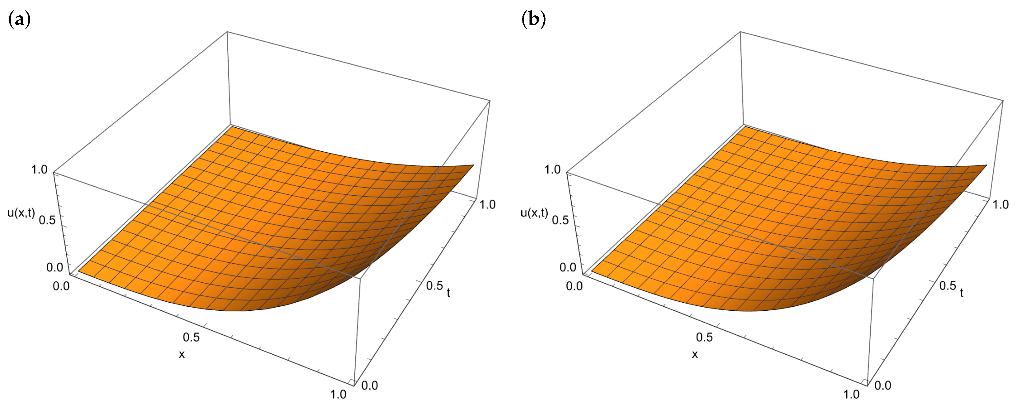
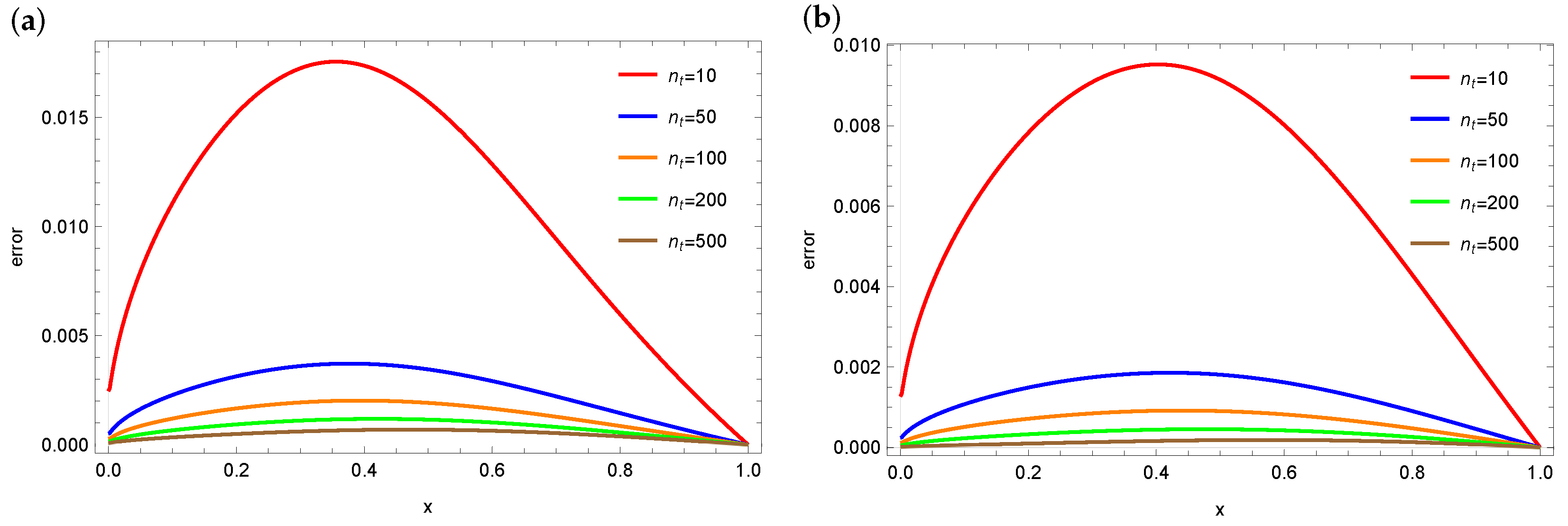
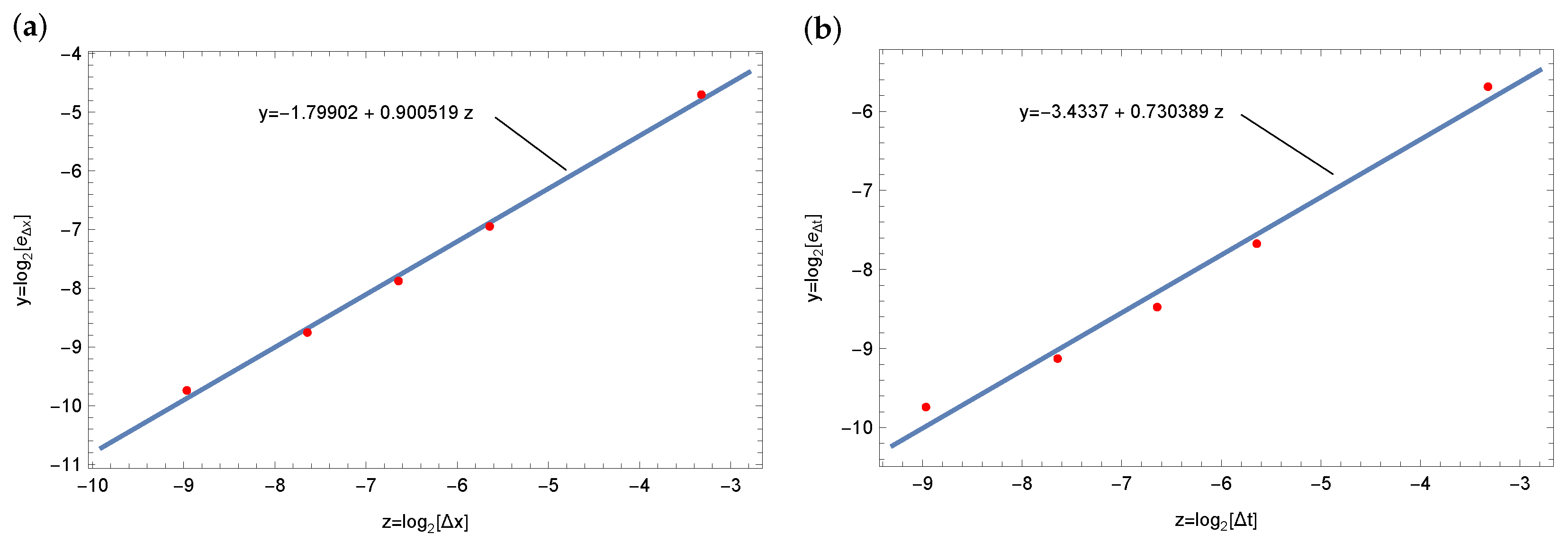
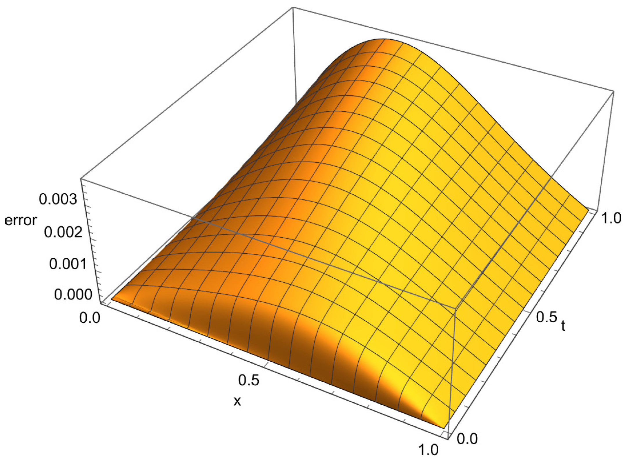
4. Numerical Calculations

4.1. Example 1

The following data appearing in Equation (1) are assumed in the considered example: $\beta =0.5$, $l_x=1$, $t^{*}=1$, $\widehat{k}\left(T\right)=2T+1$, $c\left(T\right)=T^2/5$, $\varrho \left(T\right)=T+0.3$, and

$$f(x,t)=-\frac{8}{\sqrt{\pi }}{e}^{-t}{x}^{3/2}-\frac{176}{5\sqrt{\pi }}{e}^{-2t}{x}^{9/2}-\frac{3}{50}{e}^{-3t}{x}^9-\frac{1}{5}{e}^{-4t}{x}^{12}.$$

The initial condition and boundary conditions are described by means of the functions

$${\psi }_0\left(x\right)=x^3,q\left(t\right)=0,{\phi }_b\left(t\right)=e^{-t}.$$

Thus, the example concerns the region with thermal symmetry. The above data are selected so that the exact solution of the problem is known. This solution is given by function $u_e(x,t)=e^{-t}{x}^3$.

The calculations were performed for various meshes ($n_x\times n_t$). The constant mesh over time $n_t=500$ and the variable mesh over space $n_x\in \{10,50,100,200,500\}$ were taken as the first one. Then, the mesh over space was fixed at $n_x=500$, whereas the mesh over time was changed $n_t\in \{10,50,100,200,500\}$.

Figure 1 shows the exact solution and the approximate solution obtained for the densest mesh $500\times 500$. The approximation errors are so small that the differences are not noticeable in the presented figures. However, in Figure 2a, the exact solution for $x=0.5$ and the approximate solutions obtained for different densities of mesh over space are compared. The errors of the presented approximate solutions are plotted in Figure 2b. In the case of the sparsest mesh ($n_x=10$), the maximum error is equal to $0.0385$; for $n_x=50$, it decreases to the value of $0.0081$; for $n_x=100$, it takes the value of $0.0042$; for $n_x=200$, it is equal to $0.0023$; and finally, it is $0.0011$ for $n_x=500$.

Figure 1. Exact solution (a) and approximate solution for the $500\times 500$ mesh (b).

Figure 2. Exact solution for $x=0.5$ and approximate solutions obtained for various mesh densities over space (a) together with errors of these approximations (b).

In turn, Figure 3 presents the errors of approximate solutions for cross-sections $t=0.25$ and $t=0.5$ obtained for different mesh densities over space. For the sparsest mesh ($n_x=10$), the maximum error is at the level of $0.02013$ for $t=0.25$ and $0.00955$ for $t=0.5$. As the mesh becomes more dense over space, these errors decrease. For the densest mesh ($n_x=500$), they are equal to $0.00076$ and $0.00048$, respectively.

Figure 3. Errors of approximate solutions for $t=0.25$ (a) and for $t=0.5$ (b) obtained for various mesh densities over space.

Figure 4 illustrates the approximation errors for the cross-sections $t=0.3$ and $t=1$ obtained for different meshes over time. For $t=0.3$, the maximum error decreases from the value of $0.01756$ for the mesh $n_t=10$ to the value of $0.00069$ for $n_t=500$. In the case of $t=1$, the maximum obtained errors are smaller, and they decrease from the value of $0.00952$ to the value of $0.00019$, respectively.

Figure 4. Errors of approximate solutions for $t=0.3$ (a) and for $t=1.0$ (b) obtained for various mesh densities over time.

Table 1 and Table 2 show the maximum and mean absolute errors calculated for the entire region. Table 1 contains the results for various meshes over space, while Table 2 presents the results for various meshes over time. In the case of various meshes over space, the maximum error determined for the entire region decreases from the value of $3.85\times {10}^{-2}$ to the value $1.17\times {10}^{-3}$. Whereas, the mean errors decrease from the value of $8.03\times {10}^{-3}$ to the value of $3.64\times {10}^{-4}$. Next, in the case of various meshes over time, the maximum error decreases from the value of $1.94\times {10}^{-2}$ to the same value as above. Similarly, the mean error decreases from the value of $8.35\times {10}^{-2}$ to the same value as for the various meshes over space. This is the obvious consequence of the fact that the last mesh ($n_x\times n_t=500\times 500$) is the same in both cases.

Table 1. Absolute errors of the solution determined for various meshes over space (mesh over time: $n_t=500$).

${\mathit{n}}_{\mathit{x}}$	Max	Mean
10	$3.85\times {10}^{-2}$	$8.03\times {10}^{-3}$
50	$8.12\times {10}^{-3}$	$1.94\times {10}^{-3}$
100	$4.26\times {10}^{-3}$	$1.07\times {10}^{-3}$
200	$2.32\times {10}^{-3}$	$6.28\times {10}^{-4}$
500	$1.17\times {10}^{-3}$	$3.64\times {10}^{-4}$

Table 2. Absolute errors of the solution determined for various meshes over time (mesh over space: $n_x=500$).

${\mathit{n}}_{\mathit{t}}$	Max	Mean
10	$1.94\times {10}^{-2}$	$8.35\times {10}^{-3}$
50	$4.90\times {10}^{-3}$	$2.00\times {10}^{-3}$
100	$2.81\times {10}^{-3}$	$1.10\times {10}^{-3}$
200	$1.79\times {10}^{-3}$	$6.42\times {10}^{-4}$
500	$1.17\times {10}^{-3}$	$3.64\times {10}^{-4}$

Figure 5 shows the experimental estimation of the convergence rate. In the case of space variable, the approximate value of $0.9$ is obtained, while in the case of time variable, the obtained convergence rate is around $0.73$. Theoretical values are correct for sufficiently small steps $\Delta x$ and $\Delta t$. Therefore, the differences between theoretical values and their estimations are most likely a consequence of excessively large steps and the approximation errors.

Figure 5. Experimental estimation of the convergence rate with respect to the space variable (a) and time variable (b).

4.2. Example 2

In the second example, the following data appearing in the Equation (1) are assumed: $\beta =0.7$, $l_x=1$, $t^{*}=1$, $\widehat{k}\left(T\right)=T^2+1$, $c\left(T\right)=2$, $\varrho \left(T\right)=T/4$, and

$$\begin{array}{c}f(x,t)=\frac{1}{10x^{7/10}}(5x^{27/10}cos\left(t\right)(sin\left(t\right)+x)-\hfill \\ -20x^2(sin\left(t\right)+x)(sin\left(t\right)+2x)\left(\frac{sin\left(t\right)}{\Gamma \left(\frac{13}{10}\right)}+\frac{2x}{\Gamma \left(\frac{23}{10}\right)}\right)-\\ \hfill -\frac{20x\left(x^2{(sin\left(t\right)+x)}^2+1\right)}{\Gamma \left(\frac{23}{10}\right)}-3\left(x^2{(sin\left(t\right)+x)}^2+1\right)\left(\frac{sin\left(t\right)}{\Gamma \left(\frac{13}{10}\right)}+\frac{2x}{\Gamma \left(\frac{23}{10}\right)}\right)).\end{array}$$

The initial condition and boundary conditions are described by the functions

$${\psi }_0\left(x\right)=x^2,{\phi }_a\left(t\right)=0,{\phi }_b\left(t\right)=1+sint.$$

The exact solution is defined, then, by the function $u_e(x,t)=x^2+xsint$.

As in the previous example, the calculations were performed for various meshes ($n_x\times n_t$). First, a constant mesh is assumed over time, that is, $n_t=500$, and the mesh density changes over space, that is, $n_x\in \{10,50,100,200,500\}$. Then, the mesh is fixed over space, that is, $n_x=500$; the mesh density changes over time, that is, $n_t\in \{10,50,100,200,500\}$. Figure 6 illustrates the distribution of absolute error obtained for the densest mesh $500\times 500$. The maximum error in the entire region is equal to $0.0037$, while the mean error is $0.00154$.

Figure 6. Error of approximate solution for the $500\times 500$ mesh.

In Table 3 and Table 4, the maximum and mean absolute errors calculated for the entire considered region are collected. Table 3 contains the results for various meshes over space, while Table 4 includes the results for various grids over time. In the case of various meshes over space, the maximum error determined for the whole investigated region decreases from the value $2.02\times {10}^{-1}$ to the value $3.7\times {10}^{-3}$. Whereas, the mean error decreases from the level $6.51\times {10}^{-2}$ to the level $1.54\times {10}^{-3}$. Considering the case of different meshes over time, the maximum error reduces from the value of $2.75\times {10}^{-2}$ to the same value as above. Similarly, the mean error reduces from the level of $1.28\times {10}^{-2}$ to the same level as for the various mesh densities over space.

Table 3. Absolute errors of the solution determined for various meshes over space (mesh over time: $n_t=500$).

${\mathit{n}}_{\mathit{x}}$	Max	Mean
10	$2.02\times {10}^{-1}$	$6.51\times {10}^{-2}$
50	$3.47\times {10}^{-2}$	$1.32\times {10}^{-2}$
100	$1.72\times {10}^{-2}$	$6.74\times {10}^{-3}$
200	$8.73\times {10}^{-3}$	$3.50\times {10}^{-3}$
500	$3.70\times {10}^{-3}$	$1.54\times {10}^{-3}$

Table 4. Absolute errors of the solution determined for various meshes over time (mesh over space: $n_x=500$).

${\mathit{n}}_{\mathit{t}}$	Max	Mean
10	$2.75\times {10}^{-2}$	$1.28\times {10}^{-2}$
50	$7.33\times {10}^{-3}$	$3.63\times {10}^{-3}$
100	$5.24\times {10}^{-3}$	$2.47\times {10}^{-3}$
200	$4.27\times {10}^{-3}$	$1.89\times {10}^{-3}$
500	$3.70\times {10}^{-3}$	$1.54\times {10}^{-3}$

Figure 7a shows the exact solution for $x=0.3$ and the approximate solutions obtained for various mesh densities over space. The errors of the presented approximate solutions are displayed in Figure 7b. In the case of the sparsest mesh ($n_x=10$), the maximum error is equal to $0.1846$; for $n_x=50$, it decreases to the value $0.0338$; for $n_x=100$, the maximum error takes the value $0.0169$; for $n_x=200$, it is equal to $0.0086$; and finally, the maximum error is at the level of $0.0036$ for the mesh $n_x=500$.

Figure 7. Exact solution for $x=0.3$ and approximate solutions obtained for various mesh densities over space (a) together with errors of these approximations (b).

However, the errors of approximate solutions for the cross-sections $t=0.5$ and $t=1$ obtained for various mesh densities over space are plotted in Figure 8. For the sparsest mesh ($n_x=10$), the maximum error is at the level of $0.1183$ for $t=0.5$ and $0.2016$ for $t=1$. As the mesh becomes more dense over space, these errors decrease. That is, for $n_x=50$, the maximum errors are equal to $0.0219$ and $0.0346$, respectively; for $n_x=100$, they take the values $0.011$ and $0.0172$; and for $n_x=200$, they are equal to $0.0057$ and $0.0087$. Finally, in the case of the densest mesh ($n_x=500$), the maximal errors of the approximate solutions are $0.0025$ and $0.0037$, respectively.

Figure 8. Errors of approximate solutions for $t=0.5$ (a) and for $t=1.0$ (b) obtained for various mesh densities over space.

Next, Figure 9 presents the approximation errors for the cross-sections $t=0.5$ and $t=1$ obtained for various meshes over time. For $t=0.5$, the maximum error decreases from the value of $0.02503$ for the mesh $n_t=10$, through the value of $0.00426$ for the mesh $n_t=100$, ultimately reaching the value of $0.00253$ for $n_t=500$. In the case of $t=1$, the obtained maximum errors are slightly larger, and they decrease, respectively, from the value of $0.0262$, through the value of $0.00524$, finally reaching the value of $0.0037$.

Figure 9. Errors of approximate solutions for $t=0.5$ (a) and for $t=1.0$ (b) obtained for various mesh densities over time.

5. Conclusions

This paper discusses the mathematical model of heat conduction applying the Riemann–Liouville fractional derivative with respect to the spatial variable. In the considered model, the material coefficients, such as specific heat, density, and thermal conductivity, depend on temperature. Mixed boundary conditions, i.e., of the first and second kind, are assumed in the examined model. If the given heat flux $q\left(t\right)=0$, then the thermal symmetry is obtained in the investigated process. Section 3 describes the numerical solution of the considered problem in the form of an implicit finite difference scheme. The computational examples, presented in Section 4, illustrate the effectiveness of the examined method. The examples are structured so that they illustrate the impact made by the density of the used mesh on the accuracy of the approximate results. The presented research shows that the elaborated approach is effective for solving this type of problem. In the case of the $200\times 500$ mesh ($n_x\times n_t$), the computation time was approximately $100$ s and the maximum absolute error in both considered examples was less than $0.009$. Taking the denser mesh, that is $500\times 500$, increased the computation time to approximately $420$ s and reduced the maximum errors to $0.0037$.

In earlier papers, the authors dealt with the reconstruction of aerothermal heating for thermal protection systems of space vehicles [18,19,20]. In the model considered there, it was assumed that the material parameters depended on temperature and the heat conduction coefficient occurred as a derivative with respect to space. In the future, the authors plan to investigate the possibility of using the model in which the internal derivative with respect to space variable will be a derivative of a fractional order. For this aim, it will be necessary to solve the direct problem described by Equation (1). The algorithm presented in the current paper will be used for this purpose.

References

- Bhangale, N.; Kachhia, K.B.; Gómez-Aguilar, J.F. Fractional viscoelastic models with Caputo generalized fractional derivative. Math. Methods Appl. Sci. 2023, 46, 7835–7846. [Google Scholar] [CrossRef]
- Azeem, M.; Farman, M.; Akgül, A.; De la Sen, M. Fractional Order Operator for Symmetric Analysis of Cancer Model on Stem Cells with Chemotherapy. Symmetry 2023, 15, 533. [Google Scholar] [CrossRef]
- Nisar, K.S.; Farman, M.; Abdel-Aty, M.; Cao, J. A review on epidemic models in sight of fractional calculus. Alex. Eng. J. 2023, 75, 81–113. [Google Scholar] [CrossRef]
- Owolabi, K.M.; Agarwal, R.P.; Pindza, E.; Bernstein, S.; Osman, M.S. Complex Turing patterns in chaotic dynamics of autocatalytic reactions with the Caputo fractional derivative. Neural Comput. Appl. 2023, 35, 11309–11335. [Google Scholar] [CrossRef]
- Kamdem, T.C.; Richard, K.G.; Béda, T. New description of the mechanical creep response of rocks by fractional derivative theory. Appl. Math. Model. 2023, 116, 624–635. [Google Scholar] [CrossRef]
- Brociek, R.; Słota, D.; Król, M.; Matula, G.; Kwaśny, W. Comparison of mathematical models with fractional derivative for the heat conduction inverse problem based on the measurements of temperature in porous aluminum. Int. J. Heat Mass Transf. 2019, 143, 118440. [Google Scholar] [CrossRef]
- D’Elia, M.; Du, Q.; Glusa, C.; Gunzburger, M.; Tian, X.; Zhou, Z. Numerical methods for nonlocal and fractional models. Acta Numer. 2020, 29, 1–124. [Google Scholar] [CrossRef]
- Odibat, Z.; Baleanu, D. Numerical simulation of initial value problems with generalized Caputo-type fractional derivatives. Appl. Numer. Math. 2020, 156, 94–105. [Google Scholar] [CrossRef]
- Hajiseyedazizi, S.N.; Samei, M.E.; Alzabut, J.; Chu, Y. On multi-step methods for singular fractional q-integro-differential equations. Open Math. 2021, 19, 1378–1405. [Google Scholar] [CrossRef]
- Błasik, M. The Implicit Numerical Method for the Radial Anomalous Subdiffusion Equation. Symmetry 2023, 15, 1642. [Google Scholar] [CrossRef]
- Hou, J.; Meng, X.; Wang, J.; Han, Y.; Yu, Y. Local Error Estimate of an L1-Finite Difference Scheme for the Multiterm Two-Dimensional Time-Fractional Reaction–Diffusion Equation with Robin Boundary Conditions. Fractal Fract. 2023, 7, 453. [Google Scholar] [CrossRef]
- Sun, H.; Chang, A.; Zhang, Y.; Chen, W. A Review on Variable-Order Fractional Differential Equations: Mathematical Foundations, Physical Models, Numerical Methods and Applications. Fract. Calc. Appl. Anal. 2019, 22, 27–59. [Google Scholar] [CrossRef]
- Khan, M.; Rasheed, A.; Anwar, M.S.; Hussain Shah, S.T. Application of fractional derivatives in a Darcy medium natural convection flow of MHD nanofluid. Ain Shams Eng. J. 2023, 14, 102093. [Google Scholar] [CrossRef]
- Terpak, J. Fractional heat conduction models and their applications. In Volume 7 Applications in Engineering, Life and Social Sciences, Part A; Baleanu, D., Lopes, A.M., Eds.; De Gruyter: Berlin, Germany; Boston, MA, USA, 2019; pp. 225–246. [Google Scholar] [CrossRef]
- Ji, C.-c.; Dai, W.; Sun, Z.-z. Numerical Schemes for Solving the Time-Fractional Dual-Phase-Lagging Heat Conduction Model in a Double-Layered Nanoscale Thin Film. J. Sci. Comput. 2019, 81, 1767–1800. [Google Scholar] [CrossRef]
- Gholizadeh, M.; Alipour, M.; Behroozifar, M. Numerical Solution of Two and Three-Dimensional Fractional Heat Conduction Equations via Bernstein Polynomials. Comput. Math. Math. Phys. 2022, 62, 1865–1884. [Google Scholar] [CrossRef]
- Kukla, S.; Siedlecka, U.; Ciesielski, M. Fractional Order Dual-Phase-Lag Model of Heat Conduction in a Composite Spherical Medium. Materials 2022, 15, 7251. [Google Scholar] [CrossRef]
- Brociek, R.; Hetmaniok, E.; Słota, D. Reconstruction of aerothermal heating for the thermal protection system of a reusable launch vehicle. Appl. Therm. Eng. 2023, 219, 119405. [Google Scholar] [CrossRef]
- Brociek, R.; Hetmaniok, E.; Napoli, C.; Capizzi, G.; Słota, D. Estimation of aerothermal heating for a thermal protection system with temperature dependent material properties. Int. J. Therm. Sci. 2023, 188, 108229. [Google Scholar] [CrossRef]
- Brociek, R.; Hetmaniok, E.; Napoli, C.; Capizzi, G.; Słota, D. Identification of aerothermal heating for thermal protection systems taking into account the thermal resistance between layers. Int. J. Heat Mass Transf. 2024, 218, 124772. [Google Scholar] [CrossRef]
- Zingales, M.; Alaimo, G. A physical description of fractional-order Fourier diffusion. In Proceedings of the ICFDA’14 International Conference on Fractional Differentiation and Its Applications 2014, Catania, Italy, 23–25 June 2014; pp. 1–6. [Google Scholar] [CrossRef]
- Povstenko, Y. Non-axisymmetric solutions to time-fractional diffusion-wave equation in an infinite cylinder. Fract. Calc. Appl. Anal. 2011, 14, 418–435. [Google Scholar] [CrossRef]
- Povstenko, Y. Fractional Thermoelasticity; Springer: Cham, Switzerland, 2015. [Google Scholar] [CrossRef]
- Hristov, J. Approximate solutions to fractional subdiffusion equations. Eur. Phys. J. Spec. Top. 2011, 193, 229–243. [Google Scholar] [CrossRef]
- Ceretani, A.; Tarzia, D. Determination of two unknown thermal coefficients through an inverse one-phase fractional Stefan problem. Fract. Calc. Appl. Anal. 2017, 20, 399–421. [Google Scholar] [CrossRef]
- Podlubny, I. Fractional Differential Equations; Academic Press: San Diego, CA, USA, 1999. [Google Scholar]
- Özişik, M. Heat Conduction; Wiley & Sons: New York, NY, USA, 1980. [Google Scholar]
- Jaluria, Y.; Torrance, K. Computational Heat Transfer; Taylor & Francis: New York, NY, USA, 2003. [Google Scholar] [CrossRef]
- Mochnacki, B.; Suchy, J. Numerical Methods in Computations of Foundry Processes; PFTA: Cracow, Poland, 1995. [Google Scholar]
- Meerschaert, M.; Tadjeran, C. Finite difference approximations for fractional advection-dispersion flow equations. J. Comput. Appl. Math. 2006, 172, 65–77. [Google Scholar] [CrossRef]
- Owolabi, K.M. Efficient numerical simulation of non-integer-order space-fractional reaction-diffusion equation via the Riemann-Liouville operator. Eur. Phys. J. Plus 2018, 133, 98. [Google Scholar] [CrossRef]
- Cai, M.; Li, C. Numerical Approaches to Fractional Integrals and Derivatives: A Review. Mathematics 2020, 8, 43. [Google Scholar] [CrossRef]
Disclaimer/Publisher’s Note: The statements, opinions and data contained in all publications are solely those of the individual author(s) and contributor(s) and not of MDPI and/or the editor(s). MDPI and/or the editor(s) disclaim responsibility for any injury to people or property resulting from any ideas, methods, instructions or products referred to in the content.  |
© 2024 by the authors. Licensee MDPI, Basel, Switzerland. This article is an open access article distributed under the terms and conditions of the Creative Commons Attribution (CC BY) license (https://creativecommons.org/licenses/by/4.0/).