Abstract
In today’s customer-centric economy, the demand for personalized products has compelled corporations to develop manufacturing processes that are more flexible, efficient, and cost-effective. Flexible job shops offer organizations the agility and cost-efficiency that traditional manufacturing processes lack. However, the dynamics of modern manufacturing, including machine breakdown and new order arrivals, introduce unpredictability and complexity. This study investigates the multiplicity dynamic flexible job shop scheduling problem (MDFJSP) with new order arrivals. To address this problem, we incorporate the fluid model to propose a fluid randomized adaptive search (FRAS) algorithm, comprising a construction phase and a local search phase. Firstly, in the construction phase, a fluid construction heuristic with an online fluid dynamic tracking policy generates high-quality initial solutions. Secondly, in the local search phase, we employ an improved tabu search procedure to enhance search efficiency in the solution space, incorporating symmetry considerations. The results of the numerical experiments demonstrate the superior effectiveness of the FRAS algorithm in solving the MDFJSP when compared to other algorithms. Specifically, the proposed algorithm demonstrates a superior quality of solution relative to existing algorithms, with an average improvement of 29.90%; and exhibits an acceleration in solution speed, with an average increase of 1.95%.
1. Introduction
The individualized requirements in the market are increasing, which is placing higher demands on manufacturing systems [1,2]. To remain competitive, companies are increasing the flexibility of their manufacturing systems [3,4]. However, flexibility in the manufacturing environment can lead to increased complexity, posing challenges for production managers when making decisions [5,6]. Industry 4.0 has led to the emergence and evolution of various technologies that support decision-making in manufacturing systems [7,8]. This enables continuous iteration and upgrading of both hardware and software in manufacturing systems. Benefiting from the support and maturity of these technologies, dynamic scheduling has become a trend of general interest for enterprises and researchers. Compared to traditional scheduling, dynamic scheduling is more adaptable [9,10,11]. Specifically, the dynamic flexible job shop scheduling problem (DFJSP) is considered more valuable than the traditional job shop scheduling problem (JSP) [12,13]. This is because it encapsulates most of the scheduling challenges of high-mix, low-volume production in modern discrete manufacturing systems. Moreover, it deals with uncertainties inherent in the production environment, such as fluctuating demand, machine downtime, and unpredictable lead times [14].
Among the various iterations of the standard DFJSP, the multiplicity dynamic flexible job shop scheduling problem (MDFJSP) stands out as particularly applicable to manufacturing systems characterized by a significant volume of identical or similar jobs that can be grouped in the production process. Industries such as semiconductor manufacturing and motorcycle component production serve as prime examples of such systems [15,16,17]. Addressing the MDFJSP can assist production managers in increasing throughput, decreasing lead times, minimizing machine downtime, and maximizing resource utilization. Enterprises can enhance their market competitiveness by effectively managing the scheduling of multiple job instances, which can increase productivity and enable prompt response to customer requirements. The literature contains extensive research on the DFJSP, but few studies have addressed the MDFJSP [18,19,20]. Ding et al. (2022) [21] proposed a fluid master-apprentice evolutionary method to address the multiplicity flexible job shop scheduling problem, and Ding et al. (2024) [22] presented a multi-policy deep reinforcement learning method for multi-objective multiplicity flexible job shop scheduling problem. But these two papers are only applicable to static scheduling problems, and are not suitable for addressing dynamic scheduling challenges.
To fill this research gap, we investigate the MDFJSP with new order arrivals. The inclusion of numerous new jobs in new orders is more indicative of actual production scenarios [23]. However, new order arrivals frequently generate numerous new positions, leading to an extensive solution space that challenges achieving high-quality solutions. The current methods, such as meta-heuristics and dispatching rules for the DFJSP, have been observed to have shortcomings in terms of time efficiency and long-term solution quality [24,25,26]. The current literature indicates that fluid models can rapidly identify near-optimal solutions in the context of multiplicity job shop scheduling. Therefore, we propose a new algorithm called the fluid randomized adaptive search (FRAS) algorithm for the MDFJSP, by incorporating a fluid model. The FRAS algorithm integrates a fluid model-based approach named the fluid construction heuristic (FCH) with the GRAS framework. The main function of the FCH in this algorithm is to optimize the initial solution. By incorporating the FCH, which captures the system’s continuous dynamics, the FRAS algorithm offers a more robust and adaptive solution approach for the MDFJSP. The results of numerical experiments prove this novel algorithm can efficiently generate high-quality scheduling schemes for the MDFJSP with varying problem scales in a reasonable computation time. This study makes the following key contributions.
- (1)
- We propose a fluid randomized adaptive search algorithm for addressing the MDFJSP, effectively bridging the existing research gap in this area.
- (2)
- A dynamic fluid model is developed for the first time to address the MDFJSP with new order arrivals.
- (3)
- The proposed FRAS algorithm surpasses existing algorithms due to two design features. Firstly, we developed a fluid construction heuristic that incorporates an online fluid dynamic tracking policy to optimize the initial solution. Secondly, we propose a tabu search procedure based on the public critical operation to enhance the efficiency of the solution space search.
The following sections of this article are structured as follows: Section 2 reviews the related papers. Section 3 describes the MDFJSP and introduces a mathematical model along with an illustrative example. Section 3 delineates the FRAS algorithm. Section 4 provides the results and analyses. Finally, we summarize this article in Section 5, and outline future directions and recommendations.
2. Literature Review
This section provides a review of the relevant work, which consists of two main parts. Due to the scarcity of research on the MDFJSP, the first part focuses on methodologies used to solve the FJSP. The second part reviews the current state of research on fluid modeling in scheduling.
2.1. Methodologies for the FJSP
To solve FJSPs, researchers have proposed various optimization strategies, including dispatching rule-based, and meta-heuristic. Even though exact solution methods can produce the optimal solution to a problem, their complexity makes it difficult to obtain viable solutions in a reasonable timeframe [27]. Dispatching rules are widely used to address FJSPs in practical production systems [28]. However, choosing a specific dispatching rule for a particular problem is complex. Therefore, numerous methods to extract and select dispatching rules for FJSPs have been presented by researchers [29]. Furthermore, many researchers have extracted dispatching rules using the genetic programming-based method to solve the DFJSP with particular constraints [30,31]. Although dispatching rules are easy to implement, they often exhibit myopic behavior, which means they may not guarantee to reach a local optimum in the long run [32].
In addition to dispatching rule-based methods, many meta-heuristics have been proposed to generate feasible and promising schedule schemes [33,34]. Meta-heuristics can achieve new near-optimal solutions by utilizing global information at each rescheduling point [35,36]. However, these methods often encounter challenges in terms of time efficiency, primarily attributed to their intricate evolutionary processes and search methods in an expansive search space [37,38,39]. This limitation hinders their application in manufacturing systems, where new disturbances may happen unexpectedly, even before a new rescheduling scheme has been established. For more information about meta-heuristic-based methods, refer to the overview literature by Xie et al. (2019) [40].
2.2. Fluid Model
The fluid model was first proposed by Chen (1993) [41] to address the dynamic scheduling challenges associated with multiple classes of fluid traffic. The fluid model method offers a robust mathematical framework for analyzing and solving job shop scheduling problems with multiplicity characteristics [42,43,44,45]. By representing the discrete scheduling problem as a continuous fluid model, researchers can gain valuable insights into system behavior by analyzing the performance measures and developing optimization techniques. Fluid models are deterministic, continuous approximations of stochastic. Several researchers have effectively employed fluid models in both static and dynamic JSP [45,46]. However, most of the existing literature works have primarily focused on addressing the JSP. When it comes to the FJSP, applying the fluid model approach becomes more challenging due to the additional complexities involved in decision-making and representation.
Because of the limited literature on the fluid model in FJSPs, we just can conduct a comprehensive analysis of the existing literature on fluid modeling in JSPs. Table 1 analyzes the application of fluid models in JSP from three key perspectives: problem type, problem scale, and objective function. Our findings indicate that fluid models are primarily used in JSP research to obtain approximate solutions in a relatively short time frame. Consequently, they are often combined with other heuristic algorithms to enhance the efficiency of the algorithmic solution. The existing research primarily concerns deterministic problems [42,44,47,48,49], with only very few papers addressing stochastic problems [45,50]. Fluid modeling can rapidly resolve large-scale problems in certain specific contexts. However, its application is contingent on certain parameters, which means that it is applicable to a limited number of practical scenarios and some scenarios are not applicable.Furthermore, a review of the existing literature reveals that most studies on fluid models are conducted in the context of JSPs with high multiplicity [43,44]. The application of the fluid model in these papers remains constrained, and the scenarios in which the fluid model is applicable are not sufficiently discussed. This represents an avenue for further exploration.
Table 1.
Literature review of fluid models in JSPs.
Despite the extensive research on DFJSPs, there is a lack of studies specifically addressing the multiplicity of characteristics of DFJSPs. This research gap highlights the need to develop an optimization model and propose an efficient solution approach for addressing the complexities introduced by multiplicity in DFJSPs. By considering the unique challenges posed by multiplicity, future research efforts can contribute to the advancement of scheduling methodologies and provide valuable insights for optimizing the performance of DFJSPs in practical manufacturing environments.
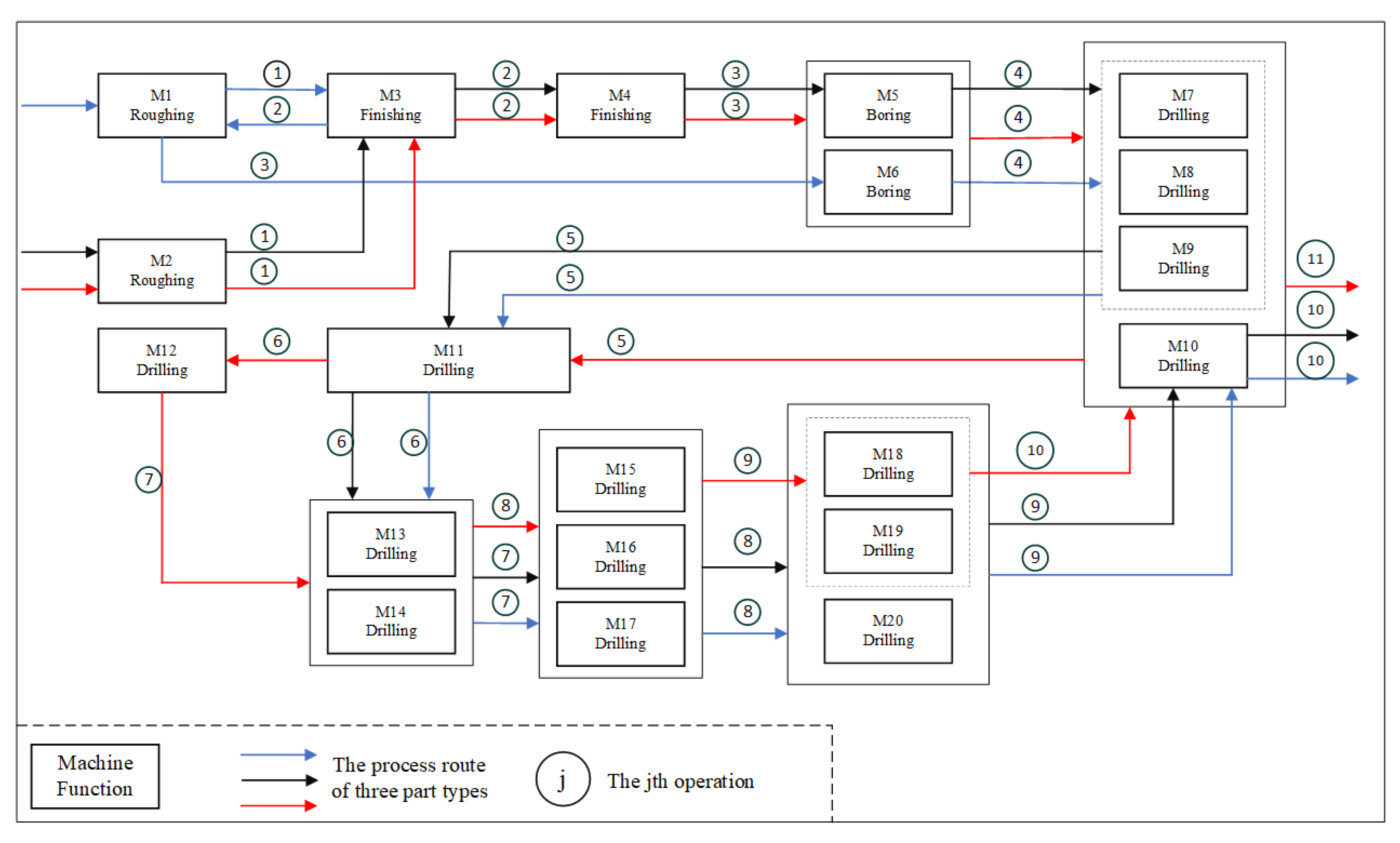
3. Problem Description
This article studies a special variant of the DFJSP called the multiplicity dynamic flexible job shop scheduling problem (MDFJSP). In MDFJSPs, multiple jobs are permitted for any job type. It consists of M machines, S orders with random arrival times, and R job types. Each job type r comprises several operations. All jobs are classified into a total of R unique types. The orders s arrive randomly, containing jobs for job type r. The job quantity belonging to a specific job type r in order s is called its multiplicity (). In the actual manufacturing environment, the arrival of new orders containing multiple jobs for each job type follows the Poisson distribution [51], which means the time interval between new orders’ arrival obeys an exponential distribution [52]. Rescheduling occurs when a new order s arrives at , serving as the rescheduling point. All operations are divided into four sets: completed, being processed, unprocessed, and new arrived operations. To handle complexity, some assumptions were made:
- (1)
- Machines are assumed to be ready for operation at the beginning of the time horizon.
- (2)
- The same type of jobs can be processed on a specified series of machines. However, it is not permitted for any given machine to perform more than one operation simultaneously.
- (3)
- Operations must be completed without interruption.
- (4)
- Operations must be conducted in a specified order, with no operation starting before the previous one has finished.
- (5)
- Setup times between operations are not considered.
The mathematical model uses the following notations:
| Notation | Description |
| Indexes: | |
| s | Orders, . |
| m | Machines, . |
| Job types, . | |
| Jobs belonging to job types r and , , . | |
| Operations of job types r and , , . | |
| Parameters: | |
| R | The number of job types. |
| M | The number of machines. |
| The operation quantity of job type r. | |
| Job of type r. | |
| Operation of the job pertaining to job type r. | |
| Operation of type r. | |
| The processing time for operation on machine m. | |
| Notation | Description |
| Sets: | |
| The complete set of machines, . | |
| The specific set of machines that are eligible to perform the operation . | |
| The set of all job types, . | |
| The set of all jobs belonging to type r, . | |
| The set of all operations belonging to job type r, . | |
| The complete set of operations belonging to all job types, . | |
| The set of operations that machine m can perform, . | |
| Variables: | |
| S | The quantity of new orders. |
| The arrival time of order s; order is the first order, and . | |
| The due date of order s. | |
| The due date of job ; if . | |
| The total job quantity of job type r in order s. | |
| The total job quantity in order s, . | |
| The total job quantity of job type r in all orders, . | |
| N | The number of jobs in all orders, . |
| The completion time of operation . | |
| Decision variables: | |
We describe the mathematical model as follows:
Subject to:
Equation (1) represents the objective of minimizing the maximum completion time in the mathematical model, where means the maximum completion time, i.e., the makespan. Equation (2) implies that the completion time of each operation is non-negative. Equation (3) indicates that each operation can be assigned to only one available machine. Equation (4) indicates that each job belongs to only one order. Equation (5) states the precedence constraint of operations for each job, while Equation (6) ensures jobs are processed only upon arrival. Equation (7) ensures that the scheduling schemes are feasible for the capacity of machines.
To facilitate comprehension for the reader, Table 2 provides an illustrative example of MDFJSP with two new orders and three machines. Initially (in order 1), each job type is allocated a specific number of available positions. The dynamic scheduling system then implements the schedule until the next order arrives. The process of dynamic scheduling is repeated until all jobs have been completed.
Table 2.
An example for the MDFJSP with 2 new orders and 3 machines.
Figure 1 presents the details of the example of the MDFJSP. Figure 1a illustrates that two task types, r = 1, 2, are processed on three machines, m = 1, 2, 3. In addition, six jobs, 11, 12, 13, 21, 22, and 23, in order one must be planned, and order two includes four new jobs, 14, 15, 24, and 25, which come at time 50. First, we establish the scheduling scheme based on the first order, as depicted in Figure 1a. At time 50, the ongoing activities 222, 122, and 113 are not halted, but rather the rescheduling procedure is initiated when order number two arrives. All non-processed operations are rescheduled following the proposed DA3C once a rescheduling process commences. Consequently, 19 operations must be scheduled for time 50 (Reschedule point). Figure 1b depicts the new schedule scheme acquired following the arrival of the second order.
Figure 1.
An example of the MDFJSP with new order arrivals.
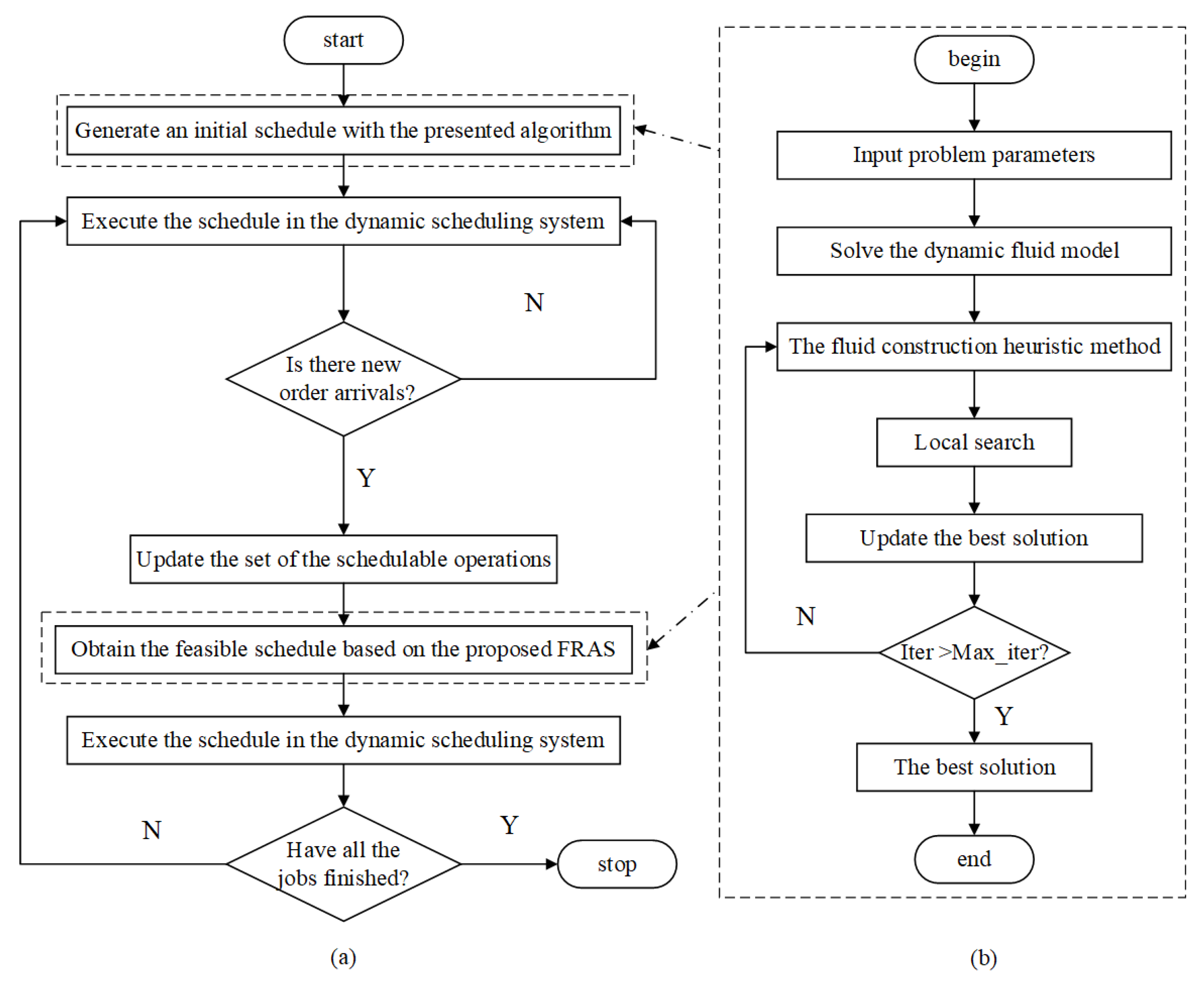
4. Fluid Randomized Adaptive Search Algorithm
In the construction phase of the fluid randomized adaptive search (FRAS) algorithm, the fluid construction heuristic (FCH) method is used to construct a solution step by step, considering symmetry. For each decision time, one operation and one corresponding available machine are selected according to the online fluid dynamic tracking policy. D solutions are constructed with the FCH. Then, the proposed tabu search procedure improves the best solution of the D solutions. Figure 2 presents the flow diagram of dynamic scheduling systems and the basic flow of the FRAS algorithm.
Figure 2.
(a) A flow diagram of the dynamic scheduling system. (b) A basic flow of the FRAS algorithm.
4.1. Construction Phase
4.1.1. Dynamic Fluid Model and Control Problem
The proposed dynamic fluid model has the advantage of being a linear programming model that can be easily solved using CPLEX. We define the solution of the fluid model as a fluid solution. The solution of the fluid model is called the fluid solution. In the dynamic fluid model, the operation is represented as fluids . Then, the set of all operations of all job types can be represented as fluid set . The dynamic fluid model provides a fluid solution, which is a time proportion that each machine devotes to each fluid. Here, we illustrate with a simple example. If machine m is equipped to perform the set of operations . After solving the fluid model, the deduced optimal time fractions that machine m spends on each operation are . The interpretation of these fractions is such that for each unit of time, , , and of that duration is allocated by machine m for performing operations , , and , respectively. The details of the dynamic fluid model are as follows:
| Notations | Description |
| Indexes: | |
| The fluid which represents the operation in the dynamic fluid model. | |
| Parameters: | |
| The processing rate of fluid on machine m. | |
| The total processing rate of fluid , . | |
| Sets: | |
| F | The set of fluids, . |
| The subset of fluids that machine m can process, . | |
| The subset of machines that can process fluid , . | |
| Variables: | |
| The proportion of processing time that machine m devotes to fluid . | |
| The completion time of fluid . | |
| The amount of fluid at time t. | |
| The job quantity in operation stage at time t. | |
| The total amount of fluid not processed at time t. | |
| The total job quantity in operation not processed at time t. | |
| The total amount of fluid not processed by machine m at time t. | |
| The total job quantity in operation not processed by machine m at time t. |
After the arrival of order s and before the arrival of order , the dynamic fluid model satisfies the following Equations (8)–(16). Obviously, the time . Equation (8) means the number of fluid at time t. The number of fluid that has not yet been processed can be calculated as Equation (9). The number of the fluid that has not yet been processed by machine m can be calculated as Equations (10) and (11). The computation time of each fluid k is shown in Equation (12). Equation (13) indicates that the utilization rate must be less than 100% for each machine. Equation (14) demonstrates that if , then the total processing rate of fluid is no more than its arrival rate. This makes , which ensures that the fluid solution is feasible. Equation (15) denotes the range of decision variables.
The dynamic fluid model aims to minimize the maximum completion time at each rescheduled point , which is shown in Equation (16).
Note that we must solve the dynamic fluid model based on both the unprocessed operations and the new operations when order s arrives at the time . Therefore, the fluid solution changes dynamically with the arrival of new orders.
4.1.2. Online Fluid Dynamic Tracking Policy
The dynamic fluid model above offers a fluid solution for each rearrangement point . The fluid solution only specifies the fraction of time devoted to a particular operation on machine m, but does not specify the job sequence for each machine. However, the dynamic flexible job shop scheduling is a process in a discrete manufacturing environment, and job sequencing must be considered along with machine assignment. Consequently, to construct high-quality discrete solutions, the fluid solution needs to transform into a policy that can guide us to finish selecting an operation and assigning it to an available machine. To generate the policy, two metrics are defined to measure the similarity between the constructed discrete and fluid solutions.
- Fluid-Gap: At time t, the gap between the total job quantity that operation has not been processed and the amount of fluid , which has not been processed, is calculated as follows:
- Fluid–Machine-Gap: At time t, the gap between the total job quantity with operation not processed by machine m and the number of fluid not processed by machine m is calculated as follows:
In Equation (17), is related to the construction state of the discrete solution at time t. The indicates a gap between the constructed discrete solution and the fluid solution. In Equation (18), , the parameter is the number of the operation that has been processed by machine m at time t. Therefore, is related to the construction state of the discrete solution at time t. The indicates a gap between the processing state of the operation on machine m in the constructed discrete solution and that in the fluid solution. Based on the two defined metrics, an online fluid dynamic tracking policy is designed, consisting of two steps: operation selection and machine selection.
In Equation (19), is the operation set that is available processed by idle machines. , is the set of idle machines, means there are jobs in the operation stage , so operation is selectable. In this step, the operation is selected randomly based on Equation (19), in which a threshold value . The parameters and are the minimum and maximum value of all operations belongs to , b is applied to balance the stochasticity and covetousness. However, due to the multiplicity of our research problem, there may be multiple jobs in the operation stage . In Equation (20), is the set of jobs in the operation stage . Therefore, the operation , which has the minimum value, is selected according to Equation (20). The job which is the first arrival operation stage is selected.
- Machine selection step: The machine is selected to process the selected operation at the operation selection step.
Based on Equation (21), where with the maximum value of is chosen to perform operation .
4.1.3. The Fluid Construction Heuristic Method
Once new order s arrives at the time , the dynamic fluid model is resolved to obtain the fluid solution. Then, the FCH is used to construct D high-quality initial solutions at the rescheduling point . Pseudo-code Algorithm 1 illustrates the detailed steps of the FCH. is the set of operations that contain the unprocessed operations and the new operations at the rescheduling point . is the set of unprocessed operations for all jobs at time t. is the set of initial solutions constructed by the FCH, in which is the ith solution.
4.2. Local Search
Tabu search has been used effectively in diverse scheduling problems since it was proposed by Glover (1990) [53]. In the local search phase of the FRAS algorithm, an improved tabu search (ITS) procedure is presented to improve the feasible solutions obtained with the FCH. In the ITS, neighborhood solutions are formed by relocating a public critical operation to a different machine and repositioning a public critical operation on the same machine. In the disjunctive graph representation of the current solution, the longest path is the critical path and each operation on the critical path is a critical operation. However, the current solution may have more than one critical path. Then, the operation is a public critical operation if it belongs to all the critical paths [54]. For example, in Figure 3, three public critical operations belong to two critical paths 111, 112, 211.
| Algorithm 1 The fluid construction heuristic method. |
|
Figure 3.
An example of public critical operations.
In the ITS, a public critical operation is reallocated on the same machine based on the neighborhood structure [55] and move a critical operation to another machine and insert it into a feasible position according to the neighborhood structure [56]. Moreover, the makespan estimate approach [56] is adopted to estimate the neighborhood quality for accelerating the local search. The procedure of the ITS is outlined in Algorithm 2.
| Algorithm 2 The improved tabu search algorithm. |
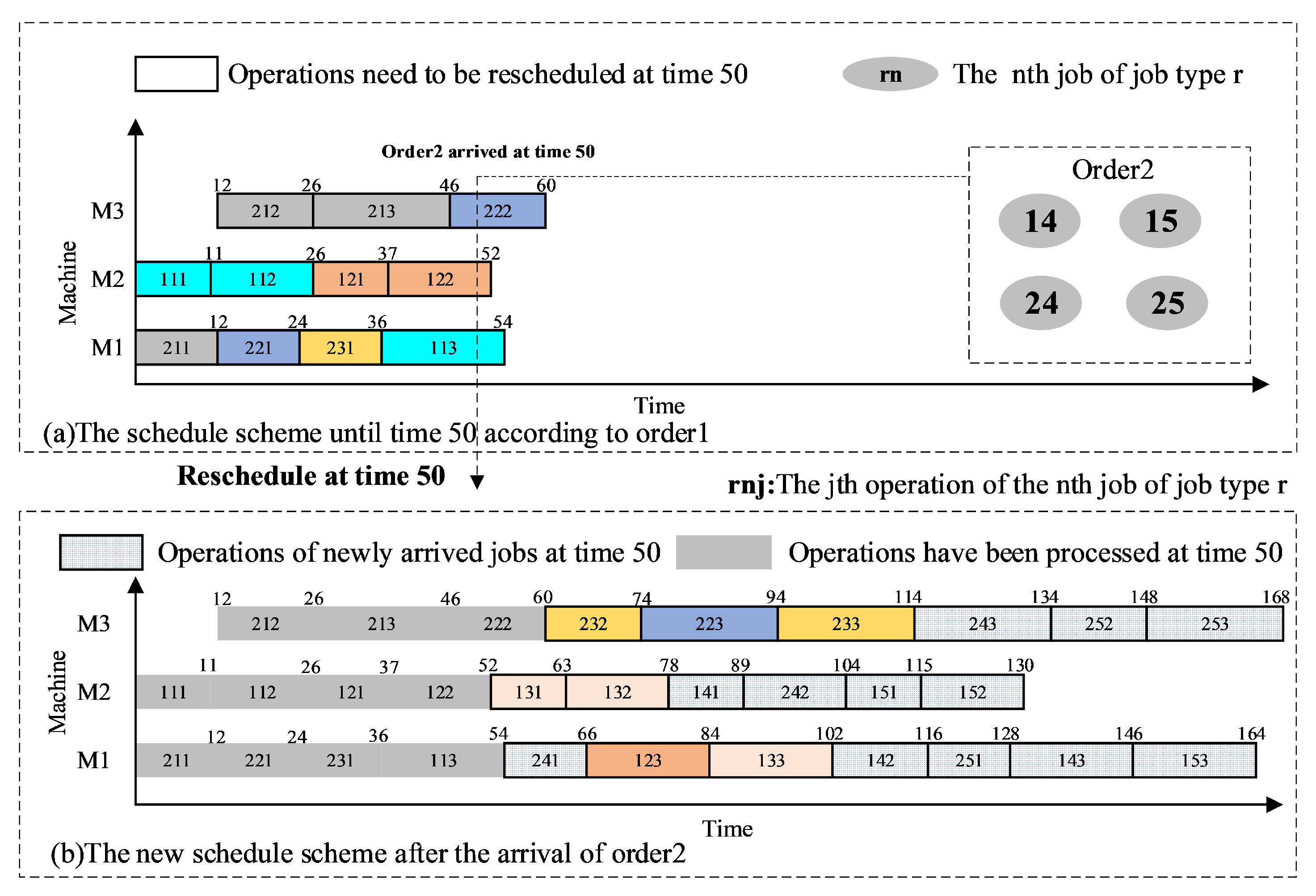
|
4.3. Implementation
Pseudo-code Algorithm 3 details the procedure of the proposed FRAS algorithm. The FRAS algorithm obtains the best solution at the rescheduling point .
| Algorithm 3 The FRAS algorithm. |
|
5. Experiments and Results
In this section, various experiments are performed to compare the efficiency and effectiveness of the FRAS algorithm. First, dynamic cases are designed to verify the performance of the FRAS algorithm. Second, the FRAS algorithm is applied to the real-world manufacturing plant case study. In practical dynamic environments, achieving satisfactory solutions quickly is crucial. Therefore, the termination condition is established as a CPU time limit of milliseconds. Here, represents the total quantity of jobs pending rescheduling at point s, M represents the count of machines, and t stands for a pre-defined constant (assigned the value of 200 in the experimental setups). All algorithms undergo 30 independent executions on each case, using a PC equipped with an Intel(R) Core(TM) i5-9300 CPU @ 2.40 GHz and 8 GB RAM, and implemented in Python 3.6. Furthermore, the MDFJSP instances () were generated based on real-world problem scenarios. Table 3 presents the generation parameters for instances. In Table 3, ‘randi’ denotes the uniform distribution of integer numbers.
Table 3.
Parameter settings for instances.
5.1. Parameter Settings
Parameter selection plays a crucial role in algorithm performance. Three parameters affect the efficiency of the proposed FRAS algorithm. In this section, we calibrate the algorithm parameters with the Taguchi method for the design of experiments (DOE) [57]. The DOE is an effective and efficient investigative method widely used to evaluate the effect of multiple factors on different algorithms. The three parameters {D, , b} define the FRAS. D is the number of generated initial feasible solutions with the FCH method for each iteration of the FRAS algorithm, is the permitted maximum iteration number with no improvement of ITS, and b is the parameter, which used to balance the stochasticity and covetousness of the proposed algorithm. Ten randomly generated instances are selected to identify the effect of the three parameters. The parameter D has four possible values: {10,20,40,80}, the parameter can be {10,20,30,40}, and the parameter b can be {0.1,0.2,0.3,0.4}. As shown in Table 4, the parameter combinations are represented with the orthogonal array . The average makespans of 10 instances, obtained through 30 independent runs of the FRAS, are used as the response values in our analysis. Figure 4 illustrates the trend in factor levels. Figure 4 shows that the FRAS algorithm with control parameters of , , and , performs better.
Table 4.
Orthogonal array and average response values.
Figure 4.
The trend of the factor level.
5.2. Validation of Proposed Methods
We conduct a set of experiments to assess the effectiveness of the proposed FCH and ITS methods in the FRAS framework for solving instances of the MDFJSP. Table 5 summarizes the experimental results. Two variants of the FRAS algorithm are considered: , which is a variant obtained by replacing the FCH with a random initialization method in the FRAS framework, and , which is a variant obtained by replacing the ITS with a classical tabu search (TS) procedure in the FRAS algorithm. The performance of these variants is compared and analyzed to assess the impact of the FCH and ITS methods in the FRAS framework.
Table 5.
Comparison of the FRAS algorithm and its variant algorithms on generated instances.
Table 5 presents data on the best and average makespan for each algorithm in the “” and “” columns, respectively. The rows labeled “#best”, “#even”, and “#worse” indicate the number of cases where the FRAS algorithm outperforms, equals, or lags behind the reference methods. The “” column indicates the average relative percentage deviation, calculated using Equation (22). Smaller values signify superior algorithm performance.
Table 5 demonstrates that the FRAS algorithm achieves the best and average makespan among all 12 instances. It outperforms FRAS_TS in 11 out of 12 instances, with FRAS_TS only achieving the best makespan for MD07. Additionally, the FRAS algorithm outperforms FRAS_RANDOM in all 12 instances. These results prove the effectiveness of the proposed FCH and ITS methods. Comparing FRAS_TS and FRAS_RANDOM, it is observed that FRAS_TS generally outperforms FRAS_RANDOM in most instances. This suggests that the FCH method has a more significant impact on improving the FRAS’s performance compared to the ITS method. Moreover, the FRAS algorithm exhibits a smaller value and displays less fluctuation in the results, indicating that the proposed methods enhance the stability and robustness of the FRAS algorithm.
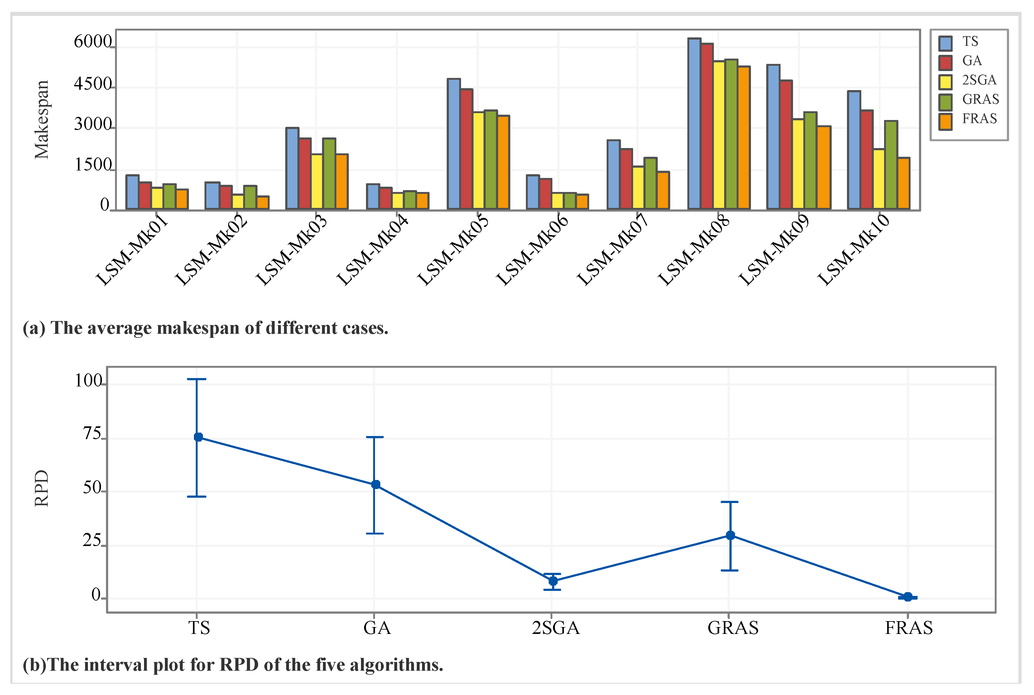
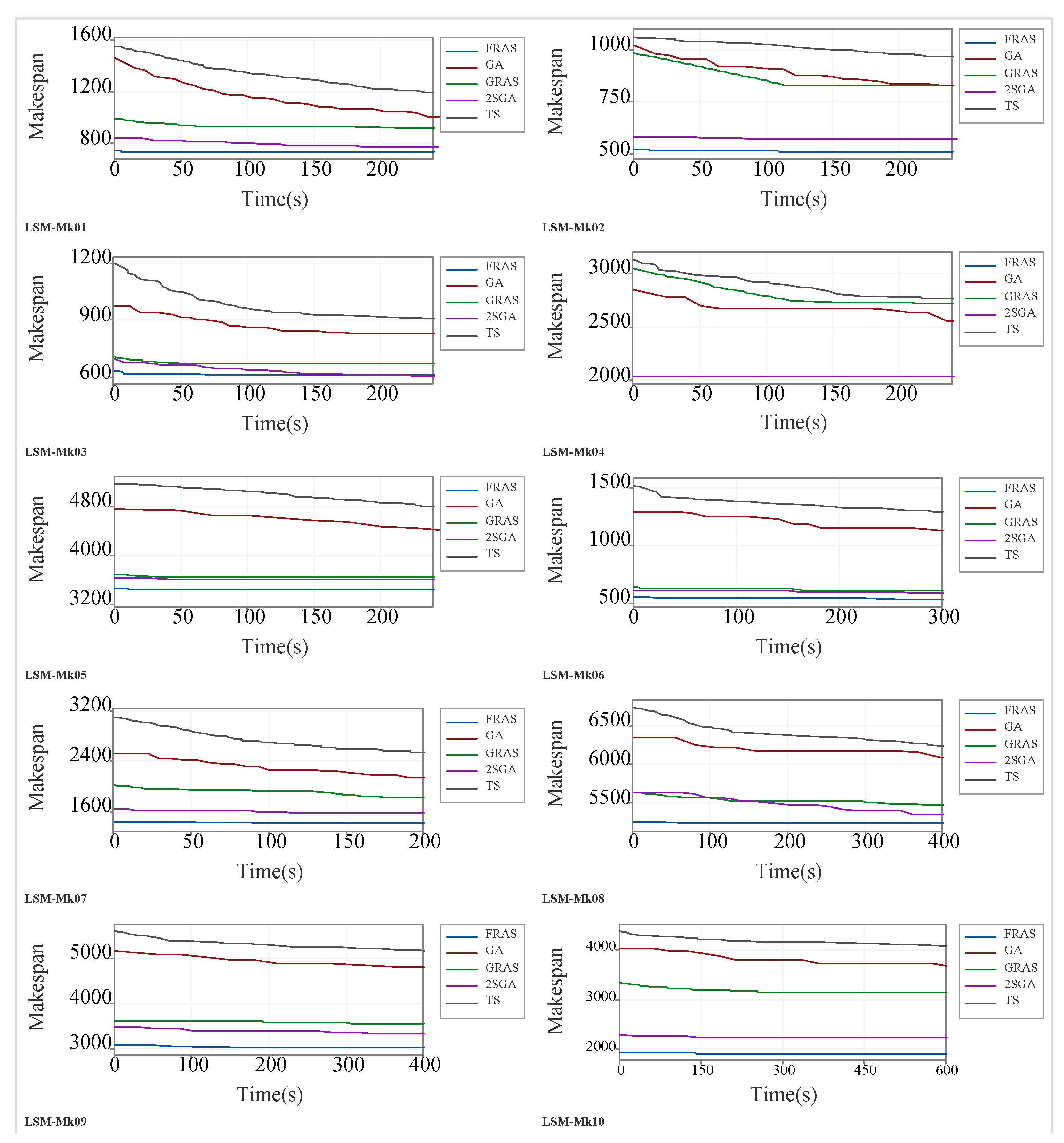
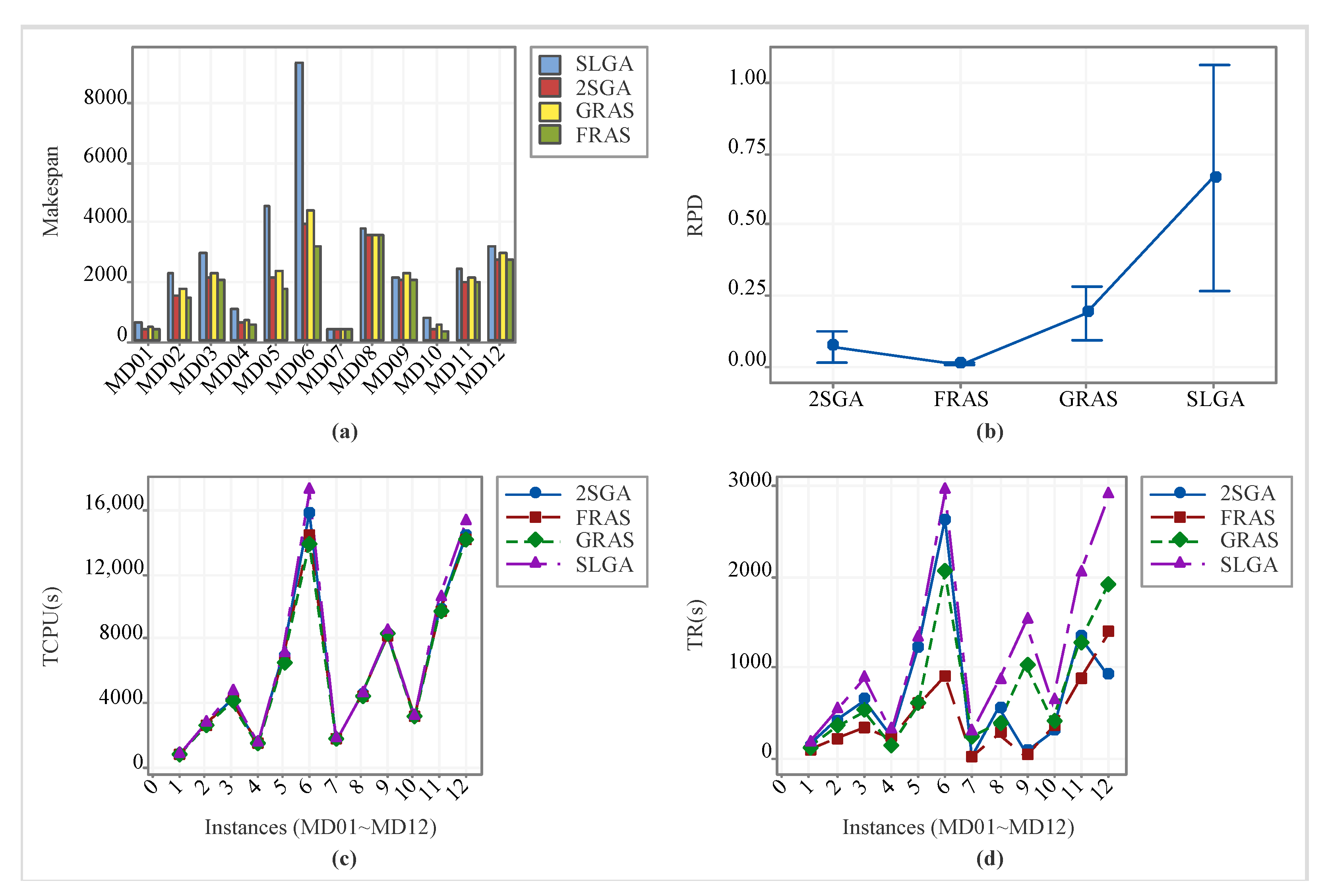
5.3. Comparison with Existing Algorithms
In this section, the FRAS algorithm is compared with the self-learning genetic algorithm (SLGA) [58], two-stage genetic algorithm (2SGA) [59], and greedy randomized adaptive search (GRAS) algorithm [38,60]. These three algorithms are utilized for solving combinatorial optimization problems. The SLGA combines Q-learning reinforcement learning methods, leading to improved performance compared to the classical genetic algorithm. The GRAS includes a successful greedy initialization method and effectively addresses FJSPs in both static and dynamic environments. The 2SGA combines fast neighborhood estimation, tabu search, and path relinking operators to successfully address FJSPs. These algorithmic approaches have demonstrated their effectiveness and efficiency in tackling complex optimization challenges in various domains. These algorithms are activated to generate a new schedule when rescheduling is triggered. The parameter settings for all comparative algorithms are selected from their corresponding literature. The respective literature has established these parameters’ values through experimental determination. Table 6 lists the result.
Table 6.
Comparison of the FRAS and reference algorithms.
Furthermore, the total computation time (TCPU) of each algorithm in every run is monitored. The TCPU represents the cumulative time expended by the algorithms across all rescheduling points. It encompasses the time taken to produce the optimal new scheduling scheme at each rescheduling point, known as the response time. Additionally, the total response time (TR) for all orders in each run is documented. Table 7 summarizes the mean TCPU and the mean TR times.
Table 7.
Comparison of the mean TCPU time and the mean TR time for the FRAS and reference algorithms.
Table 7 demonstrates that the FRAS algorithm consistently achieves the optimal solution in all 12 instances with minimal time consumption. In Figure 5b, the FRAS algorithm demonstrates the smallest value and fluctuations, indicating enhanced stability and robustness. The mean TCPU of all algorithms is depicted in Figure 5c, revealing that the four algorithms incur comparable TCPU times. Nevertheless, as shown in Figure 5d, the mean TR of the FRAS algorithm significantly outperforms the reference algorithms, making the FRAS algorithm more suitable for practical production applications, particularly in scenarios with frequent dynamic events. Moreover, the computational efficiency of the FRAS algorithm is pivotal, particularly when scaling to larger, more complex problem instances involving an increase in machines (M), job types (R), and orders (S). This growth is accompanied by an escalation in computational demand, as measured by TCPU and TR, due to the expanding and increasingly intricate solution space. The algorithm’s solution through this space necessitates more computational resources and time to secure optimal or near-optimal solutions. The influx of new orders intensifies the scheduling complexity, prompting more frequent rescheduling and a higher number of jobs to be reallocated at each rescheduling juncture. This dynamic facet of the problem amplifies the computational burden, necessitating continuous adaptation and reevaluation by the algorithm in response to evolving conditions.
Figure 5.
(a) The average makespan of different cases. (b) The interval plot for of the five algorithms. (c) The total computation time. (d) The total response time.
It is important to note that response time is essential when dealing with scheduling problems in actual manufacturing, especially when dynamic events are involved. Figure 6 presents a mean reaction time comparison for the four algorithms across all rescheduled points in four representative cases. It illustrates that the FRAS algorithm consistently exhibits shorter response times than the reference algorithms for the majority of rescheduled issues. In addition, the mean response time of the FRAS algorithm has more minor fluctuations throughout all the orders. This is owing to the addition of the FCH methods to the FRAS algorithm. The FCH constructs D solutions, and chooses the best solution as the initial solution in each iteration of the FRAS algorithm. This ensures both high quality and diversity in initial solutions. Furthermore, the FRAS algorithm maintains a well-balanced approach between exploitation and exploration capabilities through the selection of appropriate parameters and b. To statistically assess FRAS’s performance against the reference algorithms, the Wilcoxon test [61] is employed. Furthermore, we perform a sensitivity analysis to assess the impact of the time interval for new order arrivals on the algorithm’s performance. Due to space limitations, a more detailed description is provided in the Appendix D.
Figure 6.
The mean response time of the four algorithms at each rescheduling point on four represent instances.
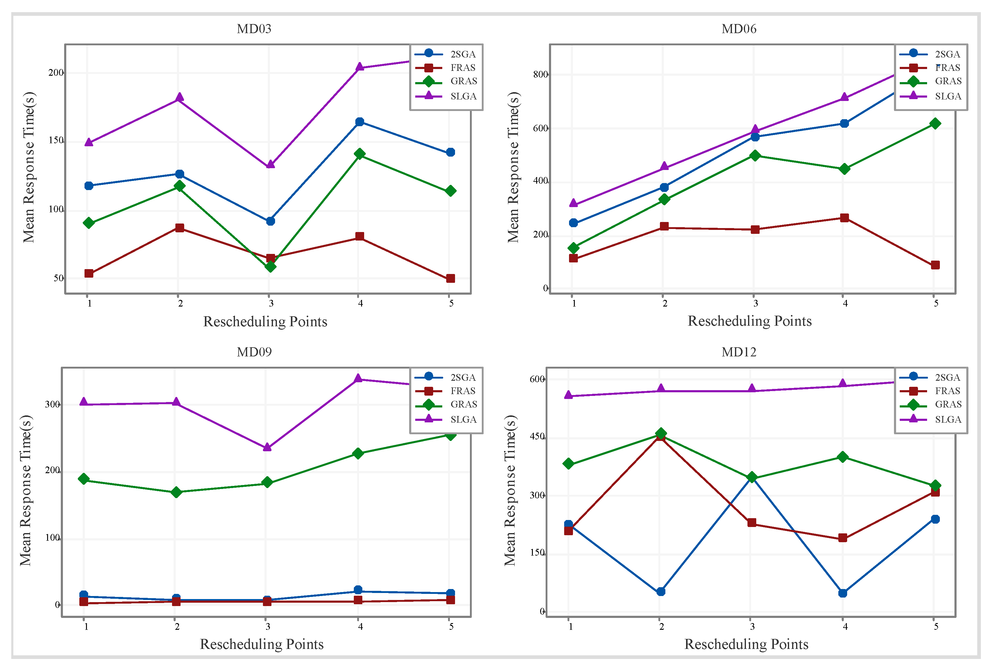
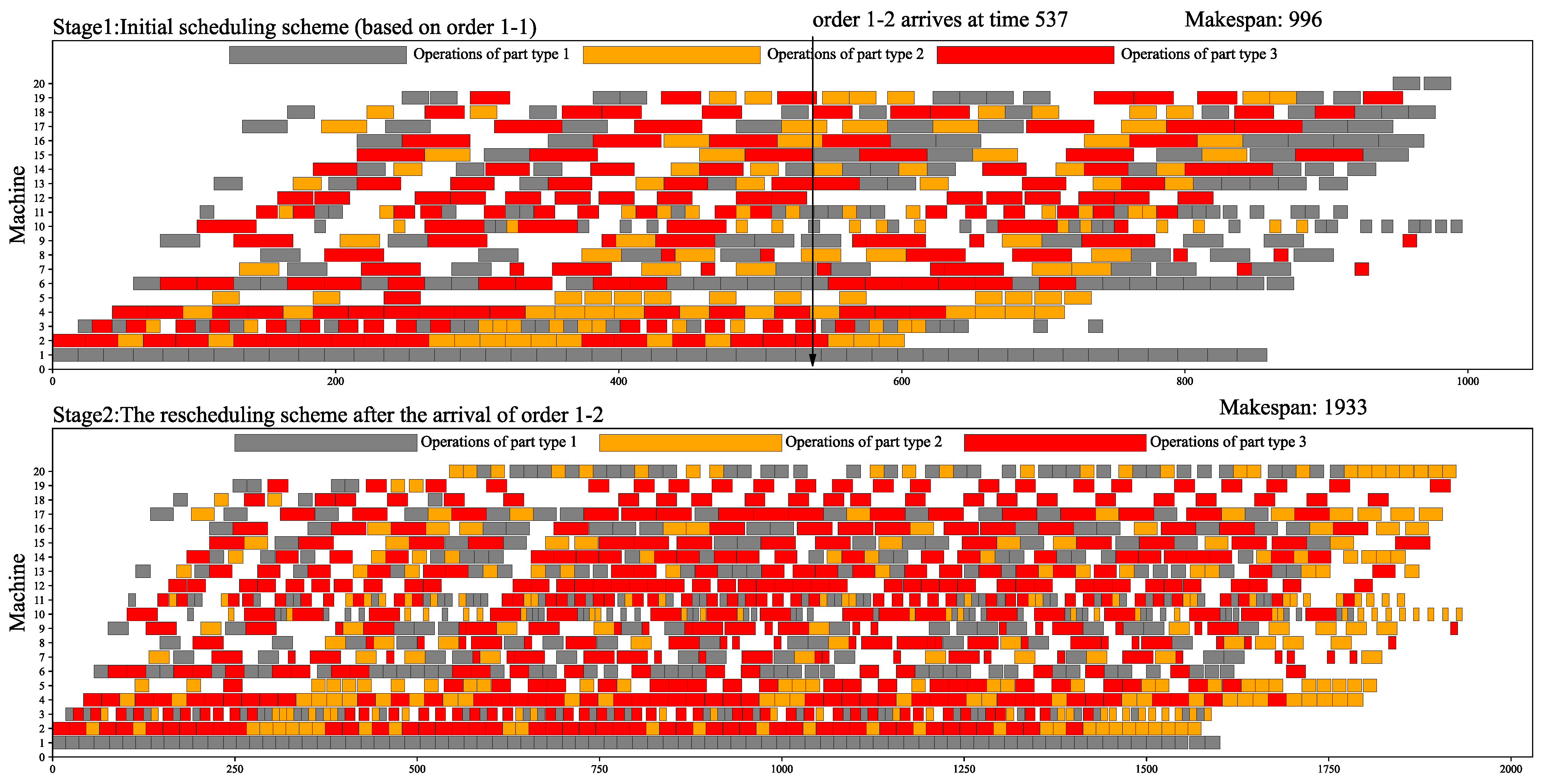
5.4. Industrial Application
To further validate the effectiveness of the FRAS algorithm, we conducted a series of practical case studies from a real-world motorcycle part manufacturing factory. The study utilizes process information obtained from a motorcycle part manufacturing factory (details in Appendix E). The manufacturing system comprises 20 machine tools, including various CNC machines, used to process 3 different types of motorcycle parts with flexible process routes as shown in Figure 7. The factory’s production data revealed the processing of hundreds of jobs daily, with orders containing multiple jobs of each part type arriving randomly. This scenario exhibits large-scale, multiplicity, and dynamic production characteristics. Five manufacturing cases (Data01–Data05) are selected based on enterprise orders, with additional information provided in Appendix E.
Figure 7.
The production process of the motorcycle parts manufacturing factory.
For instance, Data01’s initial schedule is created for orders 1-1, consisting of 51 new parts across three types, arriving at time 0 (stage 1). Subsequently, order 1-2, comprising 65 new parts and arriving at time 537, triggers the transition to the next stage (stage 2). The FRAS algorithm then generates a new schedule after orders 1-2 arrive. Figure 8 illustrates both the initial and rescheduled schemes for Data01.
Figure 8.
The initial scheduling scheme and rescheduling scheme of Data01 obtained by the FRAS algorithm.
Table 8 demonstrates that the FRAS algorithm consistently achieves optimal and average makespan results across all cases. More importantly, the FRAS algorithm exhibits significantly reduced mean total response times (TR) compared to the GRAS by from to , surpassing the other three reference algorithms by more than . These results emphasize the strong suitability of the FRAS algorithm for tackling the MDFJSP. Additionally, the FRAS algorithm consistently outperforms the reference algorithms regarding mean TR time and completion time. This indicates that the FRAS algorithm processes all parts more efficiently and can swiftly generate new rescheduling schemes in response to dynamic events. The FRAS algorithm shows significant promise for effectively addressing practical production challenges characterized by multiplicity and dynamic flexibility in shop scheduling.
Table 8.
Comparison of the FRAS algorithm and reference algorithms on manufacturing cases.
Furthermore, the FRAS algorithm’s practical utility shines through its capacity to deliver significant advantages across a spectrum of manufacturing contexts. In high-mix, low-volume sectors, such as aerospace and automotive parts production, where customization and product diversity are paramount, the algorithm’s proficiency in orchestrating various job types enhances the scheduling efficiency, shortens lead times, and elevates customer satisfaction. In just-in-time production environments, like electronics and consumer goods, marked by elevated inventory costs and variable market needs, the FRAS algorithm’s dynamic rescheduling capabilities ensure the seamless synchronization with real-time orders, minimizing stockpiles and waste. Its rescheduling agility is equally crucial in emergency response scenarios, where it facilitates rapid realignment in the face of unexpected disruptions, such as production disturbances, aiding in the swift restoration of operations and the mitigation of losses. Furthermore, for contract manufacturing enterprises where agility and rapid response are vital, the FRAS algorithm offers a competitive edge by enabling nimble scheduling adjustments to accommodate fluctuating client requirements. In each of these settings, the FRAS algorithm’s ability to navigate complexity and adapt to changing conditions not only substantiates its theoretical underpinnings but also yields tangible benefits, making it a compelling tool for elevating operational efficiency and resilience in the manufacturing landscape.
6. Conclusions and Perspective
This article investigates the multiplicity dynamic flexible job shop scheduling problem (MDFJSP) with new order arrivals. A novel fluid randomized adaptive search (FRAS) algorithm is proposed to minimize makespan. The proposed FRAS algorithm comprises two phases. In the first phase, a fluid construction heuristic (FCH) incorporating an online fluid dynamic tracking policy is presented to generate high-quality initial solutions. In the second phase, we employ an improved tabu search to enhance the search efficiency in the solution space. The efficiency of the FRAS algorithm is validated by a comparison with its variants and . Further, the performance of the FRAS algorithm is compared with the self-learning genetic algorithm, two-stage genetic algorithm, and greedy randomized adaptive search algorithm. The results indicate that the FRAS algorithm outperformed the other algorithms in terms of effectiveness and superiority for solving the MDFJSP. Statistical analysis using the Wilcoxon test further validates FRAS’s outperformance over the reference algorithms. However, the FRAS algorithm exhibits a prolonged computational time when addressing large-scale problems, rendering it unsuitable for the efficient response requirements in large-scale optimization problems.
In the future, researchers could explore multi-objective approaches for MDFJSPs. Furthermore, expanding the problem scope to incorporate machine breakdowns and changes in due dates would provide valuable insights for addressing real-world complexities.
Author Contributions
Conceptualization, L.D.; methodology, L.D., D.L. and W.F.; software, L.D.; validation, L.D. and W.F.; formal analysis, L.D., D.L. and M.R.; investigation, D.L.; writing—original draft, D.L.; writing—review and editing, Z.G., D.L., M.R. and W.F.; supervision, Z.G.; project administration, Z.G.; funding acquisition, M.R. All authors have read and agreed to the published version of the manuscript.
Funding
This work was supported by the National Natural Science Foundation of China (Grant No. 52275489), and the National Program on Key Basic Research Project (Grant No. 2021YFB3301902).
Data Availability Statement
The data that support the findings of this study are openly available at https://doi.org/10.5281/zenodo.8369652 (accessed on 18 May 2024).
Conflicts of Interest
The authors declare no conflicts of interest.
List of Abbreviations
| Abbreviation | Definition |
| JSP | Job shop scheduling problem |
| FJSP | Flexible job shop scheduling problem |
| DFJSP | Dynamic flexible job shop scheduling problem |
| MDFJSP | Multiplicity dynamic flexible job shop scheduling problem |
| FRAS | Fluid randomized adaptive search |
| FCH | Fluid construction heuristic |
| ITS | Improved tabu search |
| Average relative percentage deviation | |
| 2SGA | Two-stage genetic algorithm |
| GRAS | Greedy randomized adaptive search |
| SLGA | Self-learning genetic algorithm |
| TCPU | Total computation time |
| TR | Total response time |
| TS | Tabu search |
Appendix A. Comparison with Optimal Value
This section tests the FRAS algorithm on multiplicity instances () to be compared with optimal value. The optimal values are obtained with the KNITRO 9.0.1 solver. Table A1 shows the optimal value obtained with respect to time. The KNITRO 9.0.1 solver can only optimally solve the instance with equal or less than within the limit of two hours of computation time. The best-obtained solution by the FRAS algorithm in outperforms the KNITRO with a high gap. However, the exact method is not effective for solving problems with a larger number of jobs and machines.
Table A1.
Computation results on generated instances.
Table A1.
Computation results on generated instances.
| Instance | N × M | KNITRO 9.0.1 | FRAS | |||
|---|---|---|---|---|---|---|
| Optimality Gap (%) | ||||||
| data01 | 3 × 3 | 303 | 0.34 | 0 | 303 (303) | 0.70 |
| data02 | 6 × 3 | 551 | 0.48 | 0 | 551 (553) | 1.05 |
| data03 | 6 × 5 | 370 | 0.59 | 0 | 370 (371) | 0.85 |
| data04 | 9 × 5 | 555 | 0.72 | 0 | 555 (557) | 1.19 |
| data05 | 9 × 10 | 272 | 46.76 | 0 | 272 (272.8) | 20.06 |
| data06 | 15 × 10 | 583 | 7200 | 19.68 | 394 (396.2) | 12.26 |
| data07 | 20 × 10 | 1574 | 7200 | 99.23 | 770 (772.5) | 22.88 |
| data08 | 40 × 10 | 1457 (1462.7) | 40.10 | |||
Appendix B. Experiments on Static Datasets
In this section, experiments on multiplicity static FJSP instances are conducted to have an idea about the general attitude of the proposed FRAS algorithm. Because there is no benchmark instance for multiplicity static or dynamic FJSP so far, then this article designed 10 multiplicity static FJSP instances (LSM-Mk01-LSM-Mk10) based on the static FJSP benchmark datasets () [62]. The standard benchmarks consist of a single job per job type. Therefore, each job is duplicated several times to create large-scale multiplicity instances . To further verify the efficiency of the proposed FRAS algorithm, we compared it with the tabu search algorithm (TS) [63], genetic algorithm (GA) [12], and two state-of-the-art algorithms (two-stage genetic algorithm (2SGA) [59] and greedy randomized adaptive search algorithm (GRSA) [38]). All the algorithms run 20 times independently. The results are shown in Table A2.
In Table A1, the and columns represent each algorithm’s best and average makespan. The best solutions obtained by each algorithm are shown in bold. The rows of , , and denote that the number of cases obtained by the FRAS algorithm is better, equal, and worse than the reference algorithms. The column is the average relative percentage deviation of the objective over 20 runs. Equation (A1) defines the calculation of . The and are the average and minimum makespan, respectively. The algorithm has a better performance when a smaller is obtained.
The results in Table A1 show that the FRAS algorithm obtains the best solutions in 9 out of the 10 instances. 2SGA obtains the best solution for LSM-Mk03 and LSM-Mk04. Therefore, the FRAS algorithm has a better performance than the reference algorithms on the best solution.
Table A2.
Comparison of the FRAS and reference algorithms on generated static instances.
Table A2.
Comparison of the FRAS and reference algorithms on generated static instances.
| Instance | R | TS | GA | 2SGA | GRAS | FRAS | |||||||
|---|---|---|---|---|---|---|---|---|---|---|---|---|---|
| LSM-Mk01 | 10 | 20 | 200 × 6 | 1212 (1241) | 69.54 | 1024 (1025) | 40.03 | 782 (784) | 7.10 | 941 (942) | 28.69 | 732 (732) | 0.00 |
| LSM-Mk02 | 10 | 20 | 200 × 6 | 973 (999) | 95.12 | 840 (851) | 66.21 | 567 (570) | 11.33 | 836 (847) | 65.43 | 512 (512) | 0.00 |
| LSM-Mk03 | 15 | 10 | 150 × 8 | 2780 (2984) | 46.27 | 2555 (2595) | 27.21 | 2040 (2040) | 0.00 | 2545 (2625) | 28.68 | 2040 (2047) | 0.34 |
| LSM-Mk04 | 15 | 10 | 150 × 8 | 889 (929) | 52.80 | 780 (781) | 28.45 | 608 (608) | 0.00 | 687 (692) | 13.82 | 617 (622) | 2.30 |
| LSM-Mk05 | 15 | 20 | 300 × 4 | 4687 (4782) | 39.21 | 4371 (4395) | 27.95 | 3602 (3607) | 5.01 | 3628 (3655) | 6.40 | 3435 (3435) | 0.00 |
| LSM-Mk06 | 10 | 10 | 100 × 15 | 1221 (1262) | 139.02 | 1139 (1140) | 115.91 | 584 (585) | 10.80 | 617 (623) | 17.99 | 528 (529) | 0.19 |
| LSM-Mk07 | 20 | 10 | 200 × 5 | 2483 (2578) | 85.33 | 2170 (2192) | 57.58 | 1559 (1565) | 12.51 | 1898 (1911) | 37.38 | 1391 (1391) | 0.00 |
| LSM-Mk08 | 20 | 10 | 200 × 10 | 6226 (6263) | 19.75 | 6056 (6075) | 16.16 | 5430 (5442) | 4.05 | 5489 (5505) | 5.26 | 5230 (5230) | 0.00 |
| LSM-Mk09 | 20 | 10 | 200 × 10 | 5274 (5294) | 74.66 | 4723 (4755) | 56.88 | 3337 (3344) | 10.33 | 3495 (3545) | 16.96 | 3031 (3036) | 0.16 |
| LSM-Mk10 | 20 | 10 | 200 × 15 | 4102 (4364) | 127.53 | 3649 (3671) | 91.40 | 2212 (2217) | 15.59 | 3217 (3228) | 68.30 | 1918 (1921) | 0.16 |
| #better | 10 | 10 | 8 | 10 | |||||||||
| #even | 0 | 0 | 1 | 0 | |||||||||
| #worse | 0 | 0 | 1 | 0 | |||||||||
Figure A1a shows that among the compared algorithms, 2SGA is the closest to the FRAS algorithm, but the FRAS algorithm is superior to 2SGA in 8 out of the 10 instances except for instance LSM-Mk03 and LSM-Mk04. Figure A1b shows the interval plot for the of the FRAS algorithm and reference algorithms (: 95%), which are used for checking whether the FRAS algorithm outperforms reference algorithms statistically. The FRAS algorithm obtains a better value and has smaller fluctuations in the results, which means it has better stability and robustness.
Figure A1.
The average makespan of different static cases and interval plot for of the five algorithms.
In Figure A2, it is not difficult to find that the convergence curve of the FRAS algorithm stays below the convergence curve of other algorithms in all instances except LSM-Mk03 and LSM-Mk04. The FRAS algorithm holds the lower iteration initial point in 9 out of the 10 instances, and the final solutions of all reference algorithms are not even better than the initial solution of the FRAS algorithm in 8 instances. This is due to the proposed FCH significantly improving the performance of the FRAS algorithm, and the FRAS algorithm occupies a competitive achievement for reaching the optima at the beginning. Moreover, the FRAS algorithm converges to the best solution faster than the reference algorithms. In general, we can conclude that the FRAS algorithm is significantly more excellent than other algorithms while solving the large-scale multiplicity static FJSPs.
Figure A2.
The mean convergence curve of LSM-Mk01-LSM-Mk10.
Appendix C. Statistical Analysis
In this section, the Wilcoxon test is used to compare the FRAS algorithm with the reference algorithms to check whether the proposed algorithm outperforms all reference algorithms statistically. The Wilcoxon is a non-parametric test method that is suitable for continuous optimization problems in multiple-problem analysis [61]. Table A3 summarizes the results of applying the Wilcoxon test on the average makespan. They display the sum of rankings obtained in each comparison and the p-value associated. The FRAS algorithm outperforms these reference algorithms considering independent pairwise comparisons due to the p-value are below . However, Wilcoxon’s test performs individual comparisons between two algorithms. If we include them within the multiple comparisons, the p-value obtained is . Then it can be deduced that HFMAE outperforms the three reference algorithms in terms of solution quality with a level of significance .
Table A3.
Wilcoxon test considering average makespan.
Table A3.
Wilcoxon test considering average makespan.
| FRAS vs. | p-Value | ||
|---|---|---|---|
| SLGA | 36 | 0 | 0.00390625 |
| 2SGA | 36 | 0 | 0.00390625 |
| GRAS | 36 | 0 | 0.00390625 |
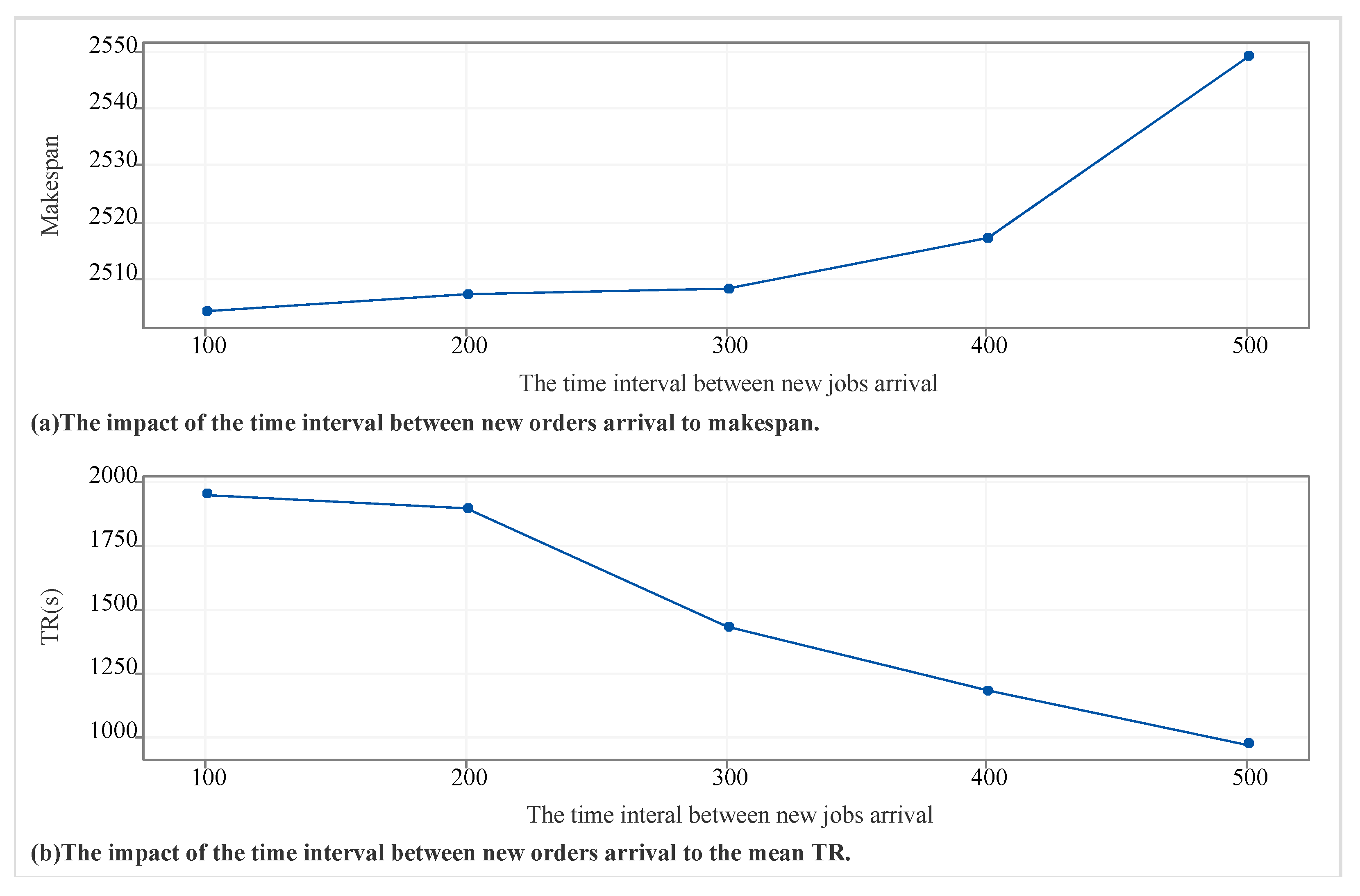
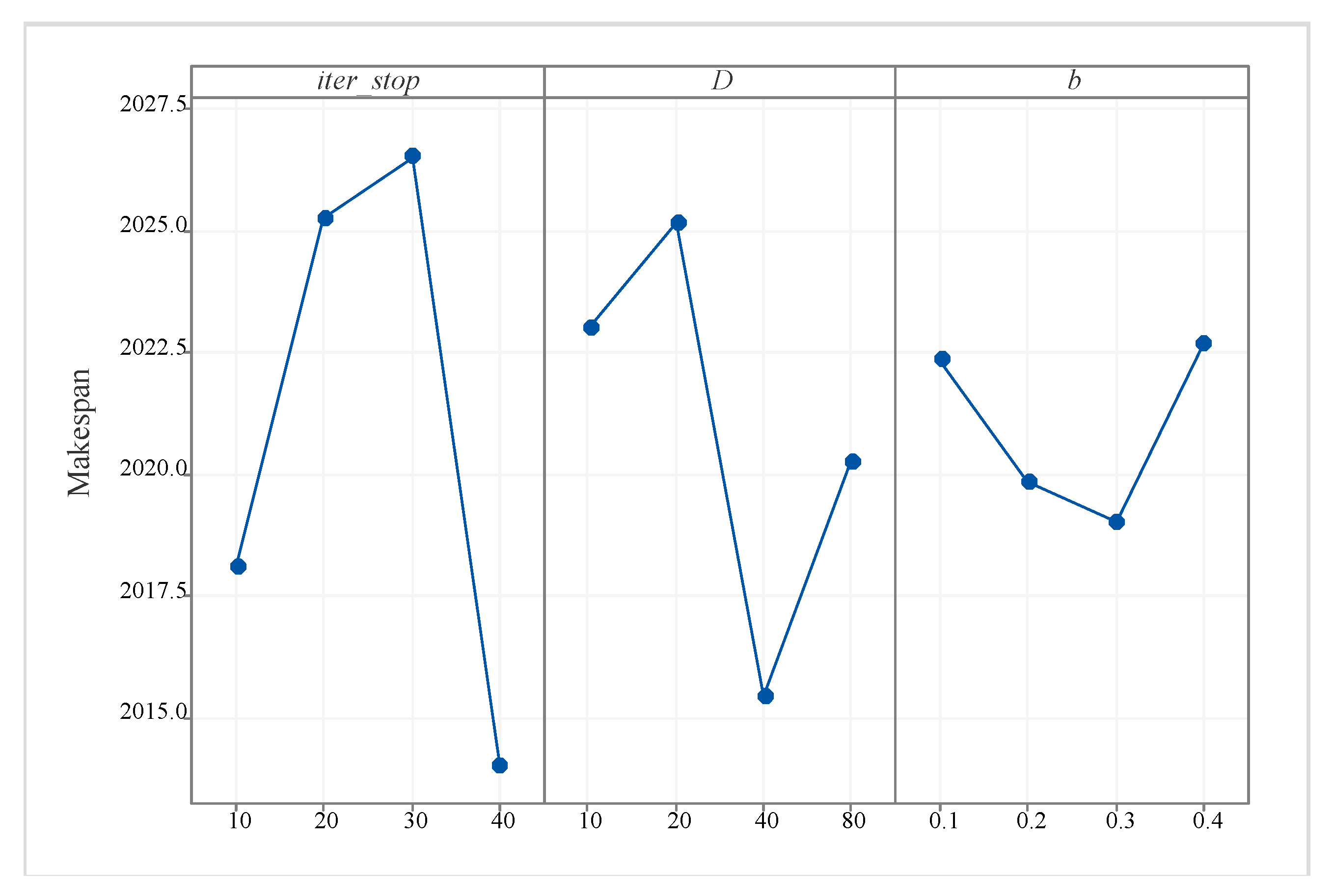
Appendix D. Sensitivity Analysis
To further assess the extent of our proposed algorithm, an instance with , , is used to perform a sensitivity analysis to analyze the impact of the time interval between new orders’ arrival on the objective and the mean total response time (TR). Figure A3 shows the results of the sensitivity analysis.
Figure A3.
The impact of the time interval between new orders’ arrival on the objective and the mean total response time (TR).
From Figure A3, it can be observed that increasing the time interval between new orders’ arrival leads to an increase in makespan and a decrease in the mean total response time. This can be explained by the fact that fewer jobs need to be rescheduled at each rescheduling point, reducing the complexity of the scheduling problem. As a result, the FRAS algorithm can converge to a final solution more quickly. Additionally, a more significant time interval between new orders’ arrival makes the scheduling system more myopic, limiting the potential for finding better overall schedules. These findings indicate that the FRAS algorithm effectively captures the impact of the time interval between new orders’ arrival on system performance. Furthermore, the proposed algorithm demonstrates a good stability and robustness across various levels of new orders’ arrival time intervals.
Appendix E. Process Information Furthermore, Production Data
Table A4.
The processing information of the three types of parts.
Table A4.
The processing information of the three types of parts.
| Part Types | Operation | Processing Time |
|---|---|---|
| r | j | |
| 1 | 1 | (1, 1, 1, 18) |
| 2 | (1, 2, 3, 10) | |
| 3 | (1, 3, 1, 21) | |
| 4 | (1, 4, 6, 19) | |
| 5 | (1, 5, 7, 28) (1, 5, 8, 28) (1, 5, 9, 28) | |
| 6 | (1, 6, 11, 10) | |
| 7 | (1, 7, 13, 20) (1, 7, 14, 20) | |
| 8 | (1, 8, 15, 32) (1, 8, 16, 32) (1, 8, 17, 32) | |
| 9 | (1, 9, 18, 19) (1, 9, 19, 19) (1, 9, 20, 19) | |
| 10 | (1, 10, 10, 8) | |
| 2 | 1 | (2, 1, 2, 18) |
| 2 | (2, 2, 3, 10) | |
| 3 | (2, 3, 4, 21) | |
| 4 | (2, 4, 5, 19) | |
| 5 | (2, 5, 7, 28) (2, 5, 8, 28) (2, 5, 9, 28) | |
| 6 | (2, 6, 11, 10) | |
| 7 | (2, 7, 13, 20) (2, 7, 14, 20) | |
| 8 | (2, 8, 15, 32) (2, 8, 16, 32) (2, 8, 17, 32) | |
| 9 | (2, 9, 18, 19) (2, 9, 19, 19) (2, 9, 20, 19) | |
| 10 | (2, 10, 10, 8) | |
| 3 | 1 | (3, 1, 2, 23) |
| 2 | (3, 2, 3, 14) | |
| 3 | (3, 3, 4, 25) | |
| 4 | (3, 4, 5, 26) (3, 4, 6, 26) | |
| 5 | (3, 5, 7, 42) (3, 5, 8, 42) (3, 5, 9, 42) (3, 5, 10, 42) | |
| 6 | (3, 6, 11, 15) | |
| 7 | (3, 7, 12, 25) | |
| 8 | (3, 8, 13, 31) (3, 8, 14, 31) | |
| 9 | (3, 9, 15, 48) (3, 9, 16, 48) (3, 9, 17, 48) | |
| 10 | (3, 10, 18, 28) (3, 10, 19, 28) | |
| 11 | (3, 11, 7, 10) (3, 11, 8, 10) (3, 11, 9, 10) (3, 11, 10, 10) |
Table A5.
The detailed information of the five cases.
Table A5.
The detailed information of the five cases.
| Cases | Orders (s) | Arrival Time () | Number of Parts for Different Types | ||
|---|---|---|---|---|---|
| Data01 | 1-1 | 0 | 22 | 13 | 16 |
| 1-2 | 537 | 19 | 17 | 29 | |
| Data02 | 2-1 | 0 | 11 | 14 | 15 |
| 2-2 | 641 | 22 | 20 | 29 | |
| 2-3 | 2537 | 12 | 16 | 11 | |
| Data03 | 3-1 | 0 | 11 | 15 | 26 |
| 3-2 | 1075 | 19 | 18 | 15 | |
| 3-3 | 1652 | 15 | 21 | 18 | |
| 3-4 | 4247 | 24 | 12 | 25 | |
| Data04 | 4-1 | 0 | 18 | 16 | 28 |
| 4-2 | 2253 | 29 | 16 | 15 | |
| 4-3 | 2885 | 19 | 19 | 28 | |
| 4-4 | 4726 | 25 | 24 | 20 | |
| 4-5 | 4937 | 11 | 12 | 11 | |
| Data05 | 5-1 | 0 | 24 | 13 | 12 |
| 5-2 | 1161 | 29 | 24 | 11 | |
| 5-3 | 3214 | 22 | 13 | 24 | |
| 5-4 | 3327 | 20 | 26 | 23 | |
| 5-5 | 3437 | 29 | 20 | 28 | |
References
- Gu, X.; Koren, Y. Mass-Individualisation–the twenty first century manufacturing paradigm. Int. J. Prod. Res. 2022, 60, 7572–7587. [Google Scholar] [CrossRef]
- Leng, J.; Zhu, X.; Huang, Z.; Li, X.; Zheng, P.; Zhou, X.; Mourtzis, D.; Wang, B.; Qi, Q.; Shao, H.; et al. Unlocking the power of industrial artificial intelligence towards Industry 5.0: Insights, pathways, and challenges. J. Manuf. Syst. 2024, 73, 349–363. [Google Scholar] [CrossRef]
- Basantes Montero, D.T.; Rea Minango, S.N.; Barzallo Núñez, D.I.; Eibar Bejarano, C.G.; Proaño López, P.D. Flexible Manufacturing System Oriented to Industry 4.0. In Proceedings of the Innovation and Research: A Driving Force for Socio-Econo-Technological Development 1st, Sangolquí, Ecuador, 1–3 September 2021; Springer: Berlin/Heidelberg, Germany, 2021; pp. 234–245. [Google Scholar]
- Margherita, E.G.; Braccini, A.M. Industry 4.0 technologies in flexible manufacturing for sustainable organizational value: Reflections from a multiple case study of Italian manufacturers. Inf. Syst. Front. 2023, 25, 995–1016. [Google Scholar] [CrossRef]
- Leng, J.; Chen, Z.; Sha, W.; Lin, Z.; Lin, J.; Liu, Q. Digital twins-based flexible operating of open architecture production line for individualized manufacturing. Adv. Eng. Inform. 2022, 53, 101676. [Google Scholar] [CrossRef]
- Zhang, W.; Xiao, J.; Liu, W.; Sui, Y.; Li, Y.; Zhang, S. Individualized requirement-driven multi-task scheduling in cloud manufacturing using an extended multifactorial evolutionary algorithm. Comput. Ind. Eng. 2023, 179, 109178. [Google Scholar] [CrossRef]
- Ghaleb, M.; Zolfagharinia, H.; Taghipour, S. Real-time production scheduling in the Industry-4.0 context: Addressing uncertainties in job arrivals and machine breakdowns. Comput. Oper. Res. 2020, 123, 105031. [Google Scholar] [CrossRef]
- Luo, D.; Thevenin, S.; Dolgui, A. A state-of-the-art on production planning in Industry 4.0. Int. J. Prod. Res. 2023, 61, 6602–6632. [Google Scholar] [CrossRef]
- Sangaiah, A.K.; Suraki, M.Y.; Sadeghilalimi, M.; Bozorgi, S.M.; Hosseinabadi, A.A.R.; Wang, J. A new meta-heuristic algorithm for solving the flexible dynamic job-shop problem with parallel machines. Symmetry 2019, 11, 165. [Google Scholar] [CrossRef]
- Zhou, J.; Zheng, L.; Fan, W. Multirobot collaborative task dynamic scheduling based on multiagent reinforcement learning with heuristic graph convolution considering robot service performance. J. Manuf. Syst. 2024, 72, 122–141. [Google Scholar] [CrossRef]
- Han, X.; Cheng, W.; Meng, L.; Zhang, B.; Gao, K.; Zhang, C.; Duan, P. A dual population collaborative genetic algorithm for solving flexible job shop scheduling problem with AGV. Swarm. Evol. Comput. 2024, 86, 101538. [Google Scholar] [CrossRef]
- Pezzella, F.; Morganti, G.; Ciaschetti, G. A genetic algorithm for the Flexible Job-shop Scheduling Problem. Comput. Oper. Res. 2008, 35, 3202–3212. [Google Scholar] [CrossRef]
- Gui, Y.; Tang, D.; Zhu, H.; Zhang, Y.; Zhang, Z. Dynamic scheduling for flexible job shop using a deep reinforcement learning approach. Comput. Ind. Eng. 2023, 180, 109255. [Google Scholar] [CrossRef]
- Tang, D.B.; Dai, M.; Salido, M.A.; Giret, A. Energy-efficient dynamic scheduling for a flexible flow shop using an improved particle swarm optimization. Comput. Ind. 2016, 81, 82–95. [Google Scholar] [CrossRef]
- Monch, L.; Fowler, J.W.; Dauzere-Peres, S.; Mason, S.J.; Rose, O. A survey of problems, solution techniques, and future challenges in scheduling semiconductor manufacturing operations. J. Sched. 2011, 14, 583–599. [Google Scholar] [CrossRef]
- Purba, H.H.; Aisyah, S.; Dewarani, R. Production capacity planning in motorcycle assembly line using CRP method at PT XYZ. In Proceedings of the IOP Conference Series: Materials Science and Engineering, Chennai, India, 16–17 September 2020; IOP Publishing: Bristol, UK, 2020; Volume 885, p. 012029. [Google Scholar]
- Han, J.H.; Lee, J.Y. Scheduling for a flow shop with waiting time constraints and missing operations in semiconductor manufacturing. Eng. Optim. 2023, 55, 1742–1759. [Google Scholar] [CrossRef]
- Zhang, F.; Mei, Y.; Nguyen, S.; Zhang, M. Evolving scheduling heuristics via genetic programming with feature selection in dynamic flexible job-shop scheduling. IEEE Trans. Cybern. 2020, 51, 1797–1811. [Google Scholar] [CrossRef] [PubMed]
- Tang, H.; Xiao, Y.; Zhang, W.; Lei, D.; Wang, J.; Xu, T. A DQL-NSGA-III algorithm for solving the flexible job shop dynamic scheduling problem. Expert Syst. Appl. 2024, 237, 121723. [Google Scholar] [CrossRef]
- Jing, X.; Yao, X.; Liu, M.; Zhou, J. Multi-agent reinforcement learning based on graph convolutional network for flexible job shop scheduling. J. Intell. Manuf. 2024, 35, 75–93. [Google Scholar] [CrossRef]
- Ding, L.; Guan, Z.; Zhang, Z.; Fang, W.; Chen, Z.; Yue, L. A hybrid fluid master–apprentice evolutionary algorithm for large-scale multiplicity flexible job-shop scheduling with sequence-dependent set-up time. Eng. Optim. 2024, 56, 54–75. [Google Scholar] [CrossRef]
- Ding, L.; Guan, Z.; Rauf, M.; Yue, L. Multi-policy deep reinforcement learning for multi-objective multiplicity flexible job shop scheduling. Swarm. Evol. Comput. 2024, 87, 101550. [Google Scholar] [CrossRef]
- Guo, C.T.; Jiang, Z.B.; Zhang, H.; Li, N. Decomposition-based classified ant colony optimization algorithm for scheduling semiconductor wafer fabrication system. Comput. Ind. Eng. 2012, 62, 141–151. [Google Scholar] [CrossRef]
- Kundakci, N.; Kulak, O. Hybrid genetic algorithms for minimizing makespan in dynamic job shop scheduling problem. Comput. Ind. Eng. 2016, 96, 31–51. [Google Scholar] [CrossRef]
- Lei, D.; Zhang, J.; Liu, H. An Adaptive Two-Class Teaching-Learning-Based Optimization for Energy-Efficient Hybrid Flow Shop Scheduling Problems with Additional Resources. Symmetry 2024, 16, 203. [Google Scholar] [CrossRef]
- Liu, J.; Sun, B.; Li, G.; Chen, Y. Multi-objective adaptive large neighbourhood search algorithm for dynamic flexible job shop schedule problem with transportation resource. Eng. Appl. Artif. Intell. 2024, 132, 107917. [Google Scholar] [CrossRef]
- Pei, Z.; Zhang, X.F.; Zheng, L.; Wan, M.Z. A column generation-based approach for proportionate flexible two-stage no-wait job shop scheduling. Int. J. Prod. Res. 2020, 58, 487–508. [Google Scholar] [CrossRef]
- Subramaniam, V.; Ramesh, T.; Lee, G.K.; Wong, Y.S.; Hong, G.S. Job shop scheduling with dynamic fuzzy selection of dispatching rules. Int. J. Adv. Manuf. Technol. 2000, 16, 759–764. [Google Scholar] [CrossRef]
- Zhang, H.; Roy, U. A semantics-based dispatching rule selection approach for job shop scheduling. J. Intell. Manuf. 2019, 30, 2759–2779. [Google Scholar] [CrossRef]
- Zhang, F.F.; Mei, Y.; Nguyen, S.; Zhang, M.J. Correlation Coefficient-Based Recombinative Guidance for Genetic Programming Hyperheuristics in Dynamic Flexible Job Shop Scheduling. IEEE Trans. Evol. Comput. 2021, 25, 552–566. [Google Scholar] [CrossRef]
- Đurasević, M.; Jakobović, D. Selection of dispatching rules evolved by genetic programming in dynamic unrelated machines scheduling based on problem characteristics. J. Comput. Sci. 2022, 61, 101649. [Google Scholar] [CrossRef]
- Holthaus, O.; Rajendran, C. Efficient jobshop dispatching rules: Further developments. Prod. Plan. Control 2010, 11, 171–178. [Google Scholar] [CrossRef]
- Ren, W.; Yan, Y.; Hu, Y.; Guan, Y. Joint optimisation for dynamic flexible job-shop scheduling problem with transportation time and resource constraints. Int. J. Prod. Res. 2021, 60, 5675–5696. [Google Scholar] [CrossRef]
- Fuladi, S.K.; Kim, C.S. Dynamic Events in the Flexible Job-Shop Scheduling Problem: Rescheduling with a Hybrid Metaheuristic Algorithm. Algorithms 2024, 17, 142. [Google Scholar] [CrossRef]
- Thi, L.M.; Mai Anh, T.T.; Van Hop, N. An improved hybrid metaheuristics and rule-based approach for flexible job-shop scheduling subject to machine breakdowns. Eng. Optim. 2023, 55, 1535–1555. [Google Scholar] [CrossRef]
- Guo, H.; Liu, J.; Wang, Y.; Zhuang, C. An improved genetic programming hyper-heuristic for the dynamic flexible job shop scheduling problem with reconfigurable manufacturing cells. J. Manuf. Syst. 2024, 74, 252–263. [Google Scholar] [CrossRef]
- Mohan, J.; Lanka, K.; Rao, A.N. A Review of Dynamic Job Shop Scheduling Techniques. Procedia Manuf. 2019, 30, 34–39. [Google Scholar] [CrossRef]
- Baykasoğlu, A.; Madenoğlu, F.S.; Hamzadayı, A. Greedy randomized adaptive search for dynamic flexible job-shop scheduling. J. Manuf. Syst. 2020, 56, 425–451. [Google Scholar] [CrossRef]
- Zhang, H.; Buchmeister, B.; Li, X.; Ojstersek, R. An Efficient Metaheuristic Algorithm for Job Shop Scheduling in a Dynamic Environment. Mathematics 2023, 11, 2336. [Google Scholar] [CrossRef]
- Xie, J.; Gao, L.; Peng, K.; Li, X.; Li, H. Review on flexible job shop scheduling. IET Collab. Intell. Manuf. 2019, 1, 67–77. [Google Scholar] [CrossRef]
- Chen, D.D.Y.H. Dynamic Scheduling of a Multiclass Fluid Network. Oper. Res. Lett. 1993, 41, 1104–1115. [Google Scholar] [CrossRef]
- Dai, J.G.; Weiss, G. A fluid heuristic for minimizing makespan in job shops. Oper. Res. 2002, 50, 692–707. [Google Scholar] [CrossRef]
- Bertsimas, D.; Gamarnik, D.; Sethuraman, J. From fluid relaxations to practical algorithms for high-multiplicity job-shop scheduling: The holding cost objective. Oper. Res. 2003, 51, 798–813. [Google Scholar] [CrossRef]
- Masin, M.; Raviv, T. Linear programming-based algorithms for the minimum makespan high multiplicity jobshop problem. J. Sched. 2014, 17, 321–338. [Google Scholar] [CrossRef]
- Gu, J.W.; Gu, M.Z.; Lu, X.W.; Zhang, Y. Asymptotically optimal policy for stochastic job shop scheduling problem to minimize makespan. J. Comb. Optim. 2018, 36, 142–161. [Google Scholar] [CrossRef]
- Bertsimas, D.; Nasrabadi, E.; Paschalidis, I.C. Robust Fluid Processing Networks. IEEE Trans. Autom. Control 2015, 60, 715–728. [Google Scholar] [CrossRef]
- Bertsimas, D.; Gamarnik, D. Asymptotically optimal algorithms for job shop scheduling and packet routing. J. Algorithms 1999, 33, 296–318. [Google Scholar] [CrossRef]
- Bertsimas, D.; Sethuraman, J. From fluid relaxations to practical algorithms for job shop scheduling: The makespan objective. Math. Program. 2002, 92, 61–102. [Google Scholar] [CrossRef]
- Nazarathy, Y.; Weiss, G. A fluid approach to large volume job shop scheduling. J. Sched. 2010, 13, 509–529. [Google Scholar] [CrossRef]
- Boudoukh, T.; Penn, M.; Weiss, G. Scheduling jobshops with some identical or similar jobs. J. Sched. 2001, 4, 177–199. [Google Scholar] [CrossRef]
- Shen, X.N.; Yao, X. Mathematical modeling and multi-objective evolutionary algorithms applied to dynamic flexible job shop scheduling problems. Inf. Sci. 2015, 298, 198–224. [Google Scholar] [CrossRef]
- Vinod, V.; Sridharan, R. Dynamic job-shop scheduling with sequence-dependent setup times: Simulation modeling and analysis. Int. J. Adv. Manuf. Technol. 2008, 36, 355–372. [Google Scholar] [CrossRef]
- Glover, F. Tabu search-part II. ORSA J. Comput. 1990, 2, 4–32. [Google Scholar] [CrossRef]
- Li, J.Q.; Pan, Q.K.; Liang, Y.C. An effective hybrid tabu search algorithm for multi-objective flexible job-shop scheduling problems. Comput. Ind. Eng. 2010, 59, 647–662. [Google Scholar] [CrossRef]
- González, M.A.; Vela, C.R.; Varela, R. Scatter search with path relinking for the flexible job shop scheduling problem. Eur. J. Oper. Res. 2015, 245, 35–45. [Google Scholar] [CrossRef]
- Kemmoé-Tchomté, S.; Lamy, D.; Tchernev, N. An effective multi-start multi-level evolutionary local search for the flexible job-shop problem. Eng. Appl. Artif. Intell. 2017, 62, 80–95. [Google Scholar] [CrossRef]
- Mandavi, S.; Shiri, M.E.; Rahnamayan, S. Metaheuristics in large-scale global continues optimization: A survey. Inf. Sci. 2015, 295, 407–428. [Google Scholar] [CrossRef]
- Chen, R.H.; Yang, B.; Li, S.; Wang, S.L. A self-learning genetic algorithm based on reinforcement learning for flexible job-shop scheduling problem. Comput. Ind. Eng. 2020, 149. [Google Scholar] [CrossRef]
- Defersha, F.M.; Rooyani, D. An efficient two-stage genetic algorithm for a flexible job-shop scheduling problem with sequence dependent attached/detached setup, machine release date and lag-time. Comput. Ind. Eng. 2020, 147. [Google Scholar] [CrossRef]
- Resende, T.A.F.M.G.C. Greedy randomized adaptive search procedures. J. Glob. Optim. 1995, 6, 109–133. [Google Scholar]
- García, S.; Molina, D.; Lozano, M.; Herrera, F. A study on the use of non-parametric tests for analyzing the evolutionary algorithms’ behaviour: A case study on the CEC’2005 special session on real parameter optimization. J. Heuristics 2009, 15, 617–644. [Google Scholar] [CrossRef]
- Brandimarte, P. Routing and scheduling in a flexible job shop by tabu search. Ann. Oper. Res. 1993, 41, 157–183. [Google Scholar] [CrossRef]
- Mastrolilli, M.; Gambardella, L.M. Effective neighbourhood functions for the flexible job shop problem. J. Sched. 2000, 3, 3–20. [Google Scholar] [CrossRef]
Disclaimer/Publisher’s Note: The statements, opinions and data contained in all publications are solely those of the individual author(s) and contributor(s) and not of MDPI and/or the editor(s). MDPI and/or the editor(s) disclaim responsibility for any injury to people or property resulting from any ideas, methods, instructions or products referred to in the content. |
© 2024 by the authors. Licensee MDPI, Basel, Switzerland. This article is an open access article distributed under the terms and conditions of the Creative Commons Attribution (CC BY) license (https://creativecommons.org/licenses/by/4.0/).