1. Introduction
Lifetime models are common statistical procedures which used in fitting and modeling survival events for numerous descriptions of lifetime datasets, particularly engineering and survival sciences. For fitting several kinds of data, many multi-parameter distributions are considered in the statistical literature in the statistical literature. In the last decades, various generated families of lifetime distributions have been introduced to model many datasets. However, a classical distribution is not appropriate to fit such sophisticated data. For this reason, the authors are motivated to obtain a novel extension of the existing distributions using numerous techniques, including adding new parameters by generalizing the distribution or mixing two or more classical distributions. These new statistical models provide greater flexibility in modeling for various applications such as engineering, biomedicine, actuarial science, medicine, insurance, and environmental fields. In this context, Chouia and Zeghdoudi [
1] introduced a new extension of Lindley distribution named the XLindley (XL) model. It is one way to describe the lifetime of a process or device, and it can be applied in several areas of study, such as medical science, lifetime, insurance, and hydrology. It can be considered a more efficient model than symmetrical models, notably normal distribution. A random variable (RV)
is said to have XL distribution if its probability density function (pdf) and survival function (sf) can be expressed, respectively, as follows:
and
In the last few decades, several researchers have given special attention to the XL distribution due to its importance in fitting skewed, asymmetric, complex, and lifetime datasets. For example, Fatima et al. [
2] provided certain properties of the Poisson Quasi XLindley distribution, and they demonstrated that it is more efficient and works better in analyzing lifetime datasets than other well-known models. Beghriche et al. [
3] proposed the inverse XLindley model by applying the inverse method, which is more appropriate in modeling mortality studies. The exponentiated XLindley model was defined by Alomair et al. [
4], who established numerous mathematical properties concerning the new distribution. A new flexible generalized XLindley model was considered by Musekwa et al. [
5]. Gemeay et al. [
6] established the modified XLindley distribution and investigated various tools for estimating the parameters.
In the context of distribution theory, the compound method is one of the most popular choices for fitting several types of datasets, such as skewed and lifetime data. It has been used in numerous domains of studies including economic, biology, actuarial, and environmental (see Abdelghani et al. [
7], Meraou et al. [
8,
9,
10,
11], and Jafari and Tahmasebi [
10]). The compound distributions are defined as the minimum or maximum of
M independent and identically distributed (i.i.d) RVs. Several authors applied this technique in their works, for example, one may refer to Mahmoudi and Jafari [
12] who introduced generalized exponential–power series models by compounding generalized exponential and power series distributions. The inverted Nadarajah–Haghighi power series distributions are considered by Ahsan-ul-Haq et al. [
13]. In the same way, the exponential Poisson model was introduced by Cancho et al. [
14], and Yousef et al. [
15] defined the unit Gompertz power series distribution and estimated the model parameter using the ranked set sampling method. It is worth motioning that the exponential (Exp) model has received considerable attention in the literature. It is efficiency in analyzing engineering, finance, and climatology phenomena. Further, The Exp model can be extensively implemented to fit the failure times of components and systems. Numerous authors applied the Exp model in numerous applications. A RV
follows the Exp distribution if its pdf and sf can be formulated by
and
Despite these advancements, when there are different kinds of datasets in survival and lifetime, many existing methods lack flexibility and may not provide the best fit. To overcome this challenge, we defined a novel distribution named the Compound Exponential XLindley (CEXL) model, and it can be used in different areas including lifetime and engineering fields. This proposed model has two parameters and is obtained by compounding the Exp and XL distributions. Let us consider the RVs
and
that are i.i.d, and assume that
. The sf of the random variable of
X is
Additionally, another objective of this study is to explore estimating the CEXL model parameters using two traditional estimation methods, such as maximum likelihood estimation, and Bayesian methods under the square error loss function. For more information about lifetime analysis and Bayesian inference, one may cite the works of Xu et al. [
16], Xu et al. [
17], Wang et al. [
18], Muqrin [
19], and Wu and Gui [
20]. Also, we construct the confidence intervals for model parameters using the approximate of the MLE method.
The remaining part of the current study is structured as given: The suggested compound model is developed and studied in
Section 2. The underlying characteristics of the CEXL distribution such as k-th moment, moment generating function, distribution of order statistics, and certain entropy measures are investigated in
Section 3. In
Section 4, we provide two estimation procedures for estimating the model parameters. We conduct some numerical simulation experiments in
Section 5 to observe the effectiveness of the proposed MLE and Bayes methods. Finally, in
Section 6, two lifetime datasets are analyzed for validation purposes. Finally concluding remarking has been obtained for this study In
Section 7.
2. Compound Exponential XLindley Model
A continuous RV
X is said to follow the proposed CEXL model with parameters
and
if its cumulative distribution function (cdf) and pdf are expressed, respectively, as follows:
and
From now on, we assume that .
It is evident that the proposed CEXL model contains a sub model as a special case. If
tends to be 0, the recommended CEXL reduces to an Exp distribution; when
approaches 0, we have an XL distribution.
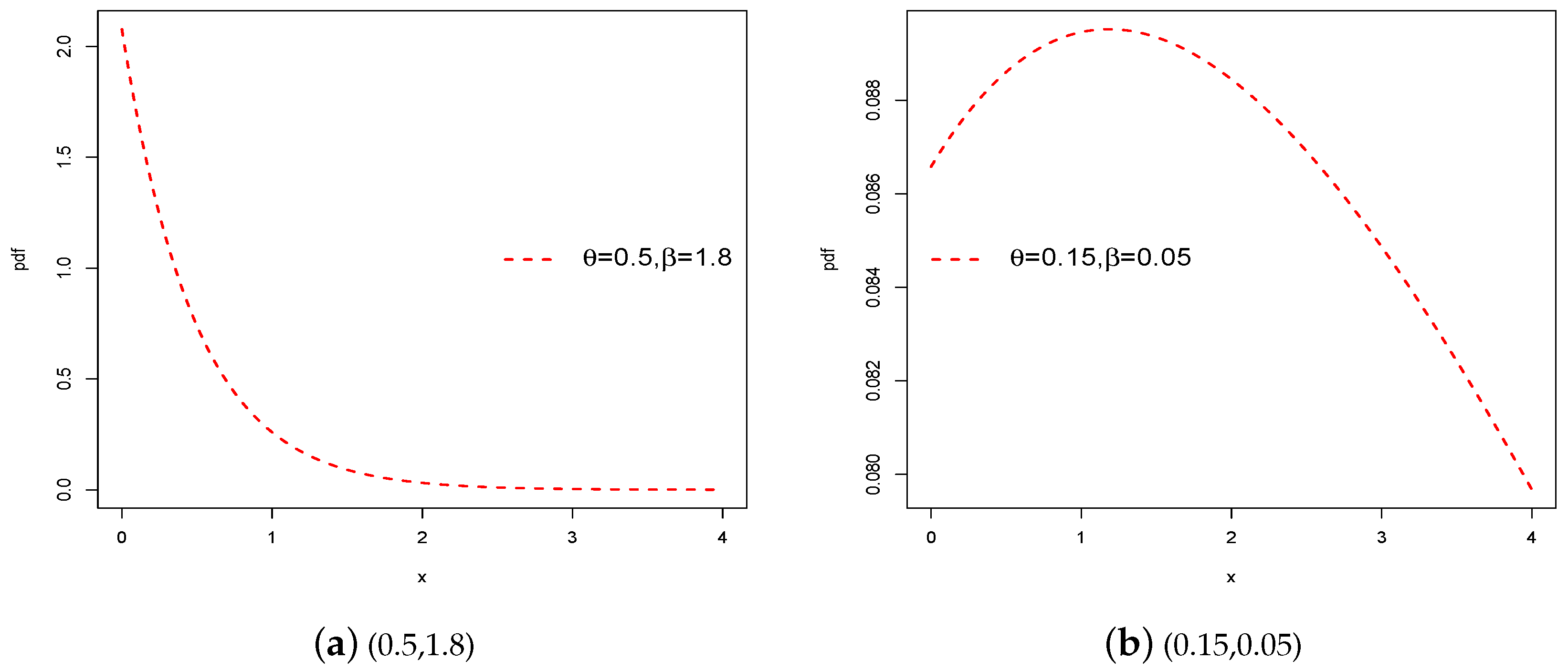
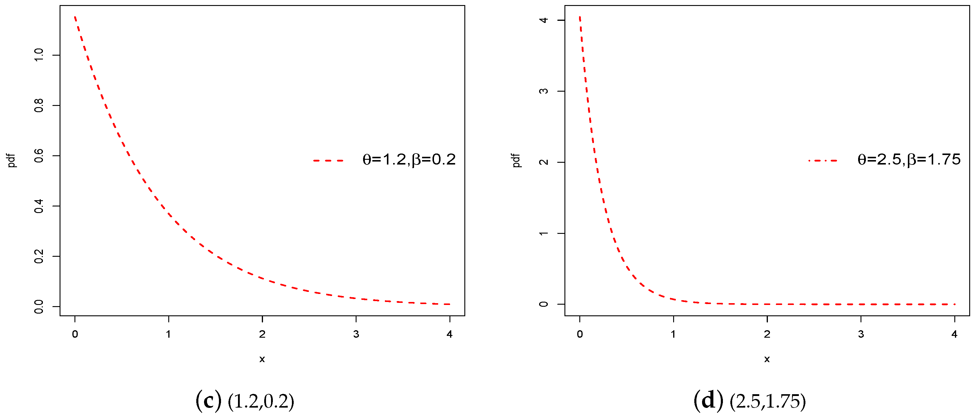
Figure 1 demonstrates the graphs for the pdf of the proposed model given in Equation (
3) using several parameters recors. It is highly positively skewed and uni-modal as well, as it is good for modeling skewed datasets.
Henceforth, the sf and hazard rate function (hrf) of the RV
X are
and
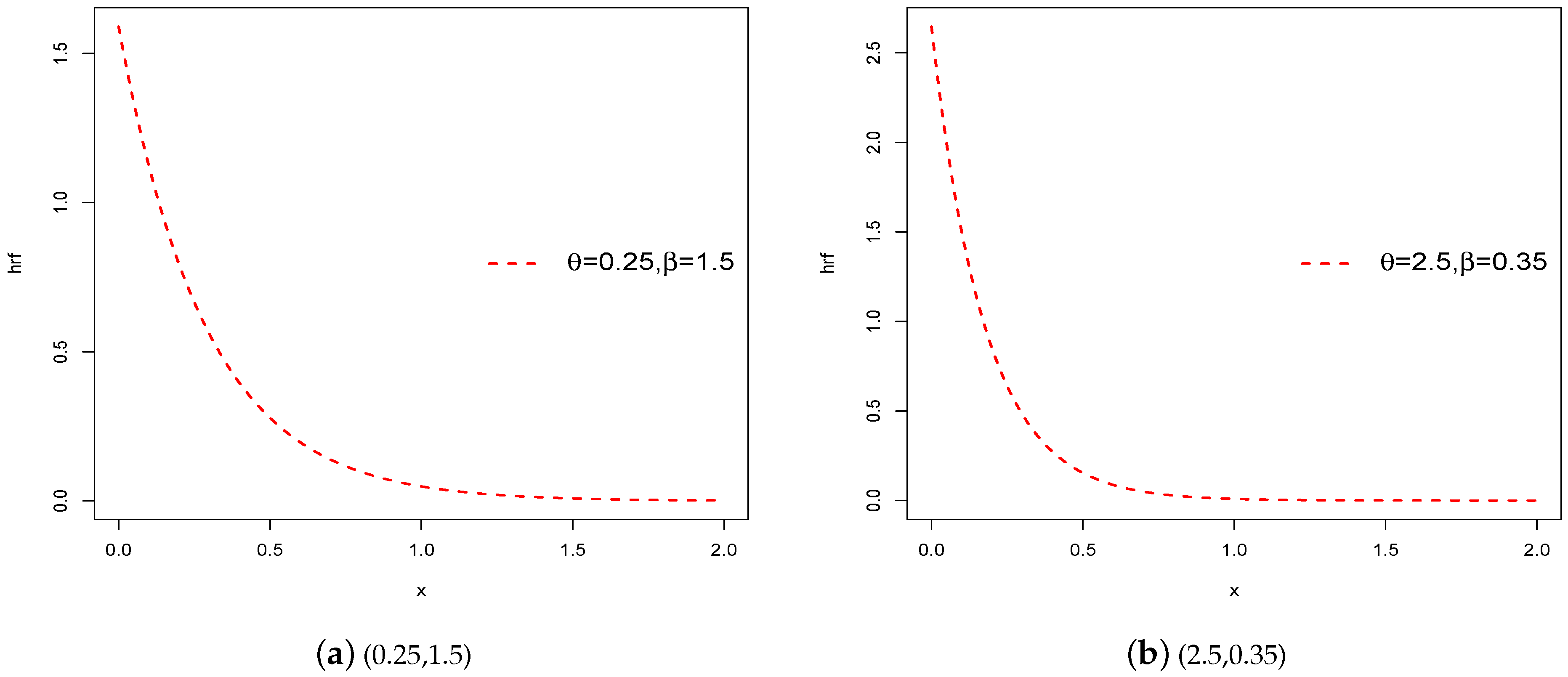
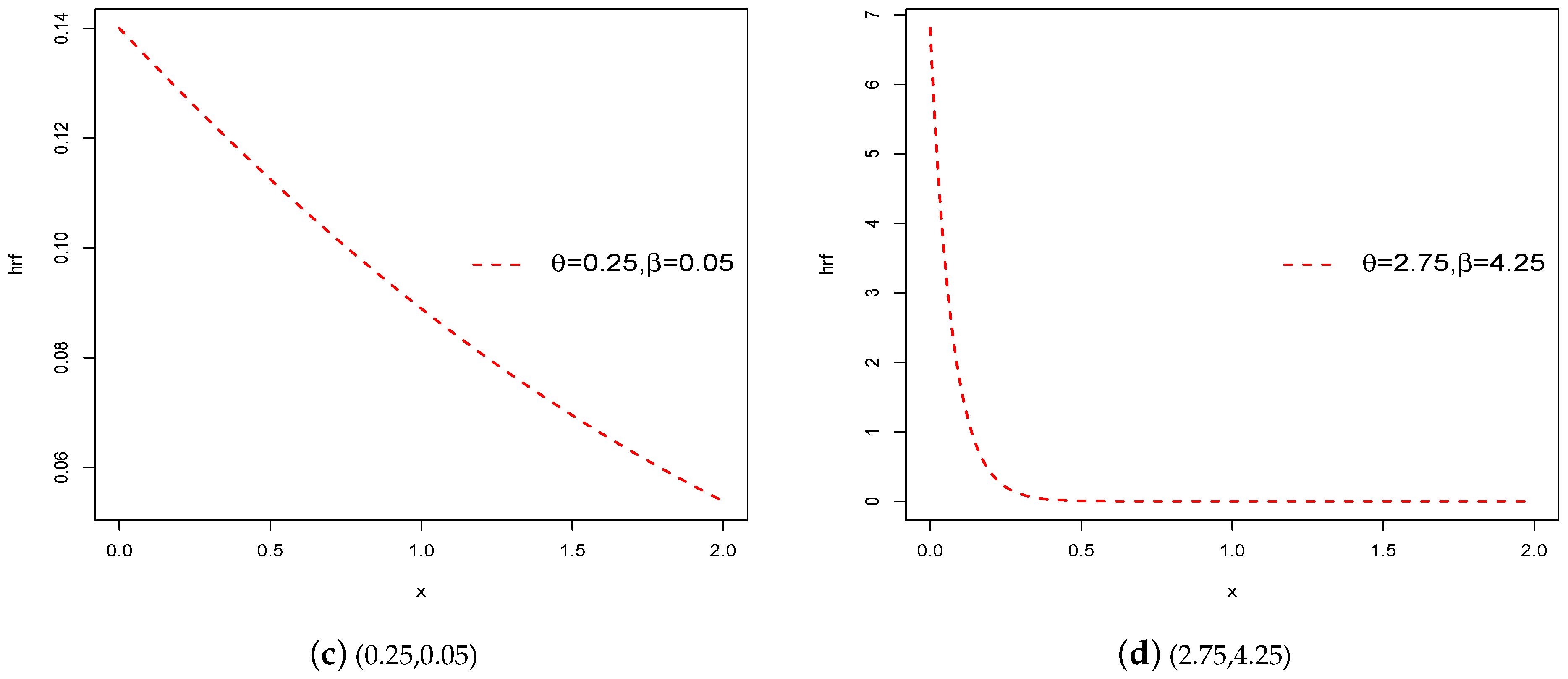
From the hrf of the CEXL model,
and
. The graphs for the hrf of the proposed model given in Equation (
4) are demonstrated in
Figure 2 for different parameter values of
and
. Clearly, for all parameter values of
and
, our CEXL distribution has a decreasing hrf, which confirms the flexibility of the recommended model.
Similarly, the cumulative hazard rate function
and inverse hazard rate function
of the RV
X are
and
The Odds function of the proposed CEXL model can be defined as the ratio of the cdf and sf. It verifies the non-monotone hrf and can be written as
3. The Characteristics of the CEXL Model
This section introduces several statistical properties of the proposed CEXL model—notably, the k-th moment, mean, variance, moment generating function, characteristic function, distribution of order statistics, and some entropy measures—because of its importance in distribution theory.
3.1. Moments with Related Measures
Let the RV
X have the CEXL model. The proposed expression k-th moment of
X is given below:
where
for
.
Proof. The expression of
k moment of
X can be defined as
□
Henceforth, the first and second moment of
X come out to be
and
The variance and coefficient of variation (CV) of
X are
and
At the end, the coefficients for skewness (
) and the kurtosis (
) of the RV
X are
and
Now, the moment generating function (mgf) and characteristic function (cf) of
X are given, respectively, below:
and
The numerical results of numerous statistical measures, as discussed previously, of the proposed CEXL model using specific parameter values are summarized in
Table 1. From these values, it can be deduced that our CEXL distribution is more efficient for explaining more datasets.
3.2. Order Statistics
We draw a random sample of size
n from the CEXL model and
represent its order statistics. The pdf of the
j-th order statistic
is expressed as follows:
The associated cdf of
is
From Equation (6), the probability distribution of maximum
and minimum
are obtained by setting
and
, respectively, and they are given as
and
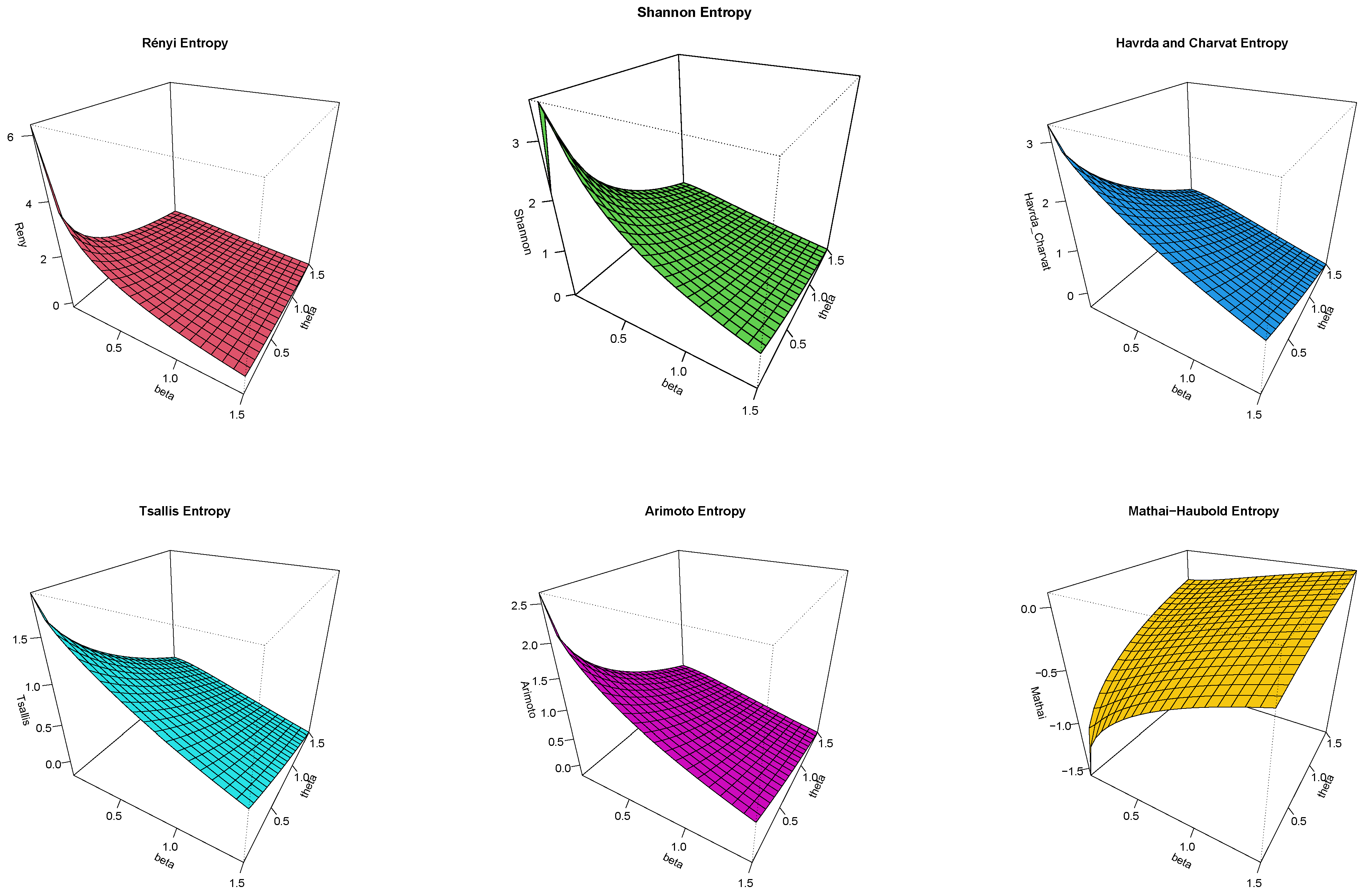
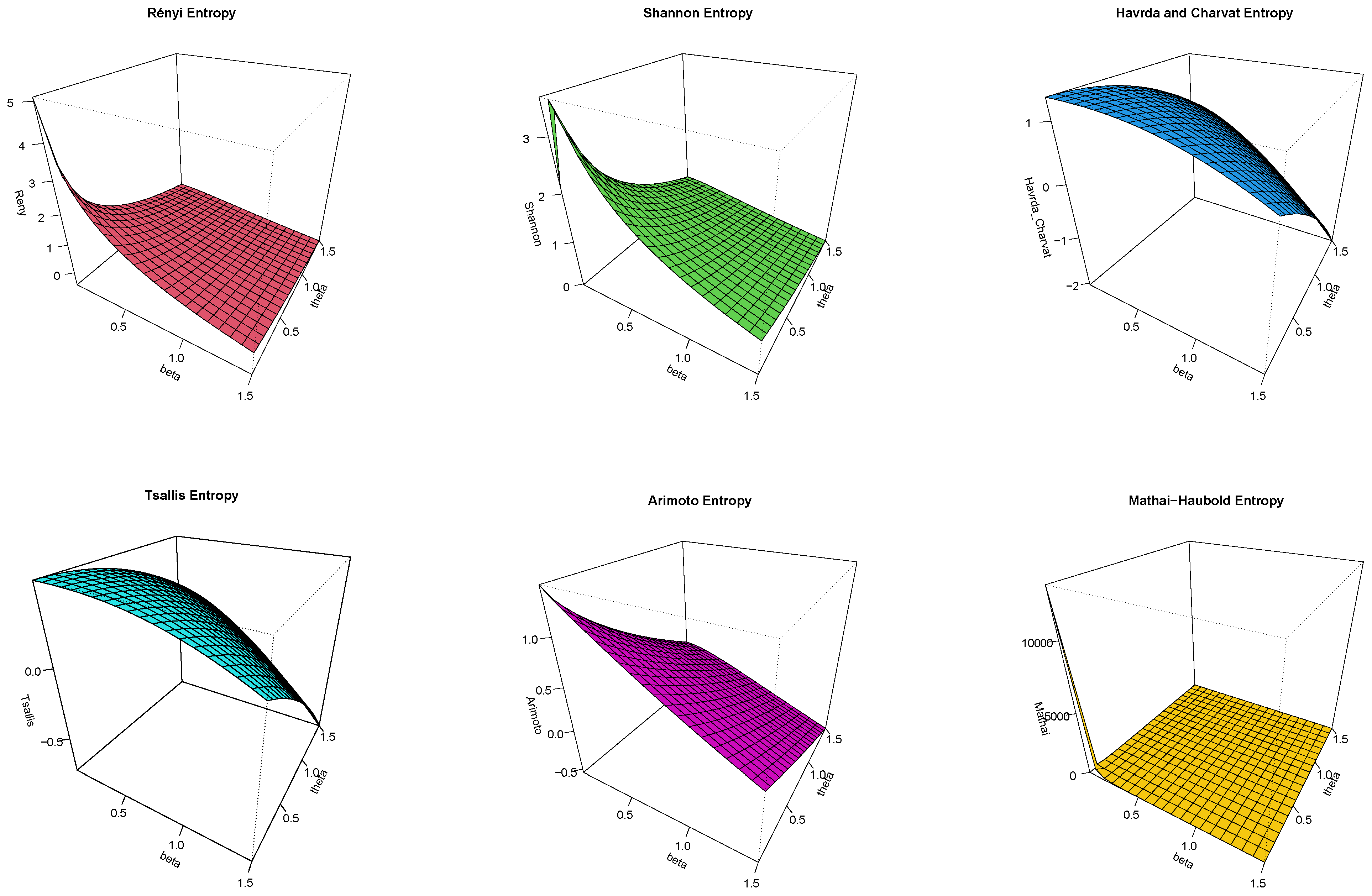
3.3. Information Measure of the CEXL Model
Here, we discuss several entropy’s such as Rényi, Shannon, Havrda and Charvat, Tsallis, Arimoto, and Mathai–Haubold. The proposed entropy measures have a key role in information amounts.
In information theory, Renyi entropy [
21]
is an important measure, and it is defined as
with
.
Shannon’s entropy [
22]
is defined as
Further, another uncertainty information measure is Havrda and Charvat entropy [
23],
, and it is expressed as
with
.
Using the proposed distribution, the Tsallis entropy [
24]
is defined as
Next, we consider the Arimoto entropy [
25]
of the recommended model, which is
Finally, a new extension entropy measure named the Mathai–Haubold entropy [
26]
is provided in this subsection. It is written as
with
.
Table 2 and
Table 3 report certain numerical values of the proposed entropy measures of the CEXL distribution by applying numerous parameter values of
and
. Also, the 3D curves of these measures are sketched in
Figure 3 and
Figure 4.
5. Simulation Study
Here, several simulation studies are conducted to demonstrate the effectiveness of the recommended estimators (MLE and Bayes estimations) for the recommended CEXL distribution. Recall that all computations are computed using R software.
We use the parameter values (Case 1 = (0.6, 1.2), Case 2 = (0.5, 1.1), and Case 3 = (0.75, 1.3)), and associated the sample sizes with 1000. For each case and under 1000 replications of the process, we draw a random sample from our CEXL model by applying the following steps of generation:
We independently generate random samples and from the U(0,1) distribution;
Compute , where denotes the cdf of exponential distribution;
Compute , where denotes the cdf of XLindley distribution;
Obtain a random sample from the proposed CEXL model as .
Henceforth, we compute the average estimate (AVEs) with its associated mean square errors (MSEs) of the unknown parameters
and
using the two procedures listed as MLE and Bayesian under several loss function methods. The results are displayed in
Table 4,
Table 5 and
Table 6.
Finally, we calculate the 95% simulated CIs for the model parameters with its average lengths (ALs) and coverage probabilities (CPs).
Table 7,
Table 8 and
Table 9 reported the obtained results.
6. Real Data Analysis
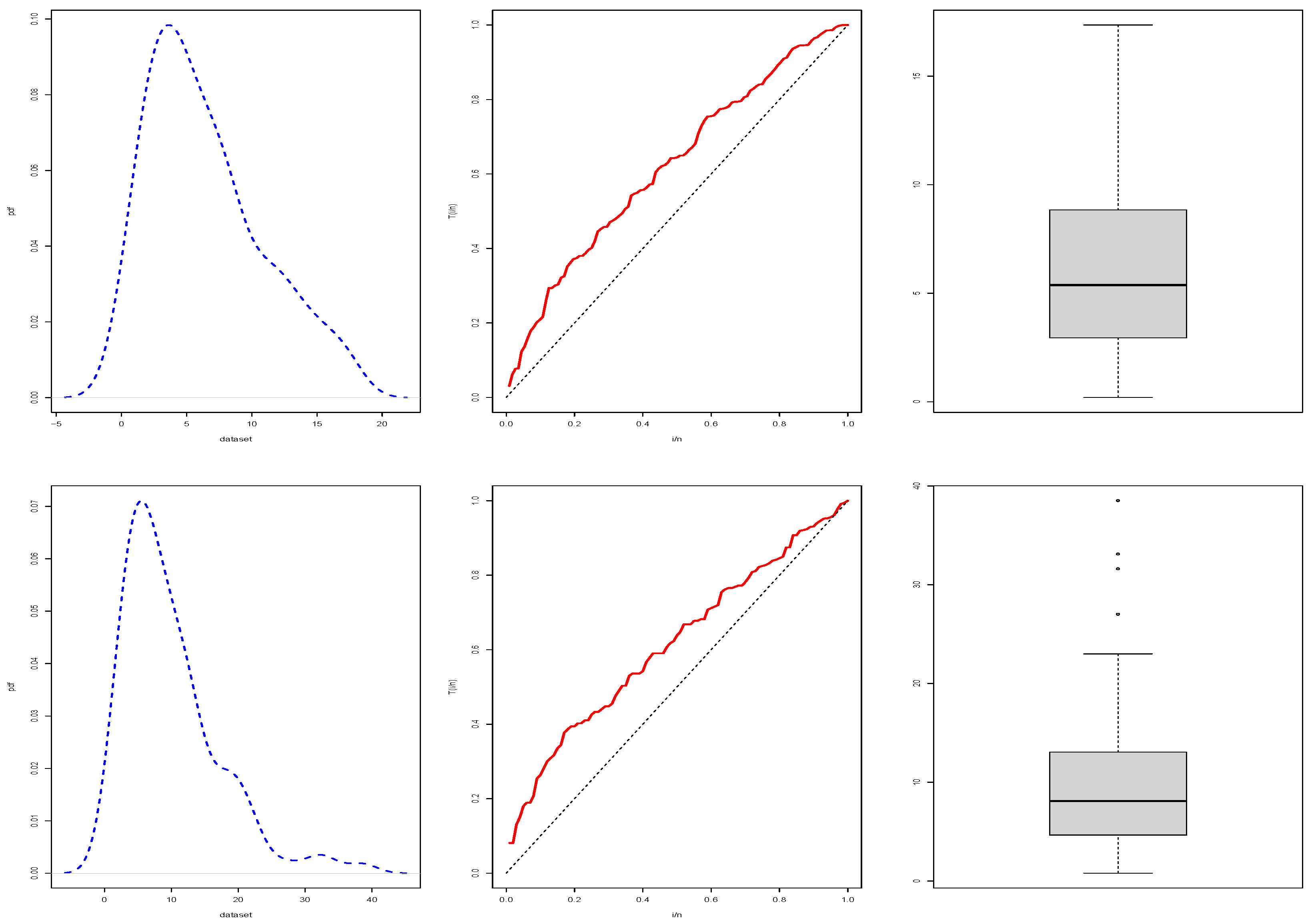
This section demonstrate the adaptability of our CEXL model using two real datasets for checking the effectiveness and performance among several well-known distributions.
The first dataset consists of the remission times of bladder cancer patients, and it was previously studied by Abouelmagd et al. [
27] and Cordeiro et al. [
28]. The observation of datasets is written in
Table 10.
The second dataset represents the waiting time (in minutes) of 100 bank customers. The considered data were studied originally by Ghitany et al. [
29] and also provided by Bhati et al. [
30]. The values of the dataset are reported in
Table 11.
The summary statistics for the proposed datasets with the kernel density, TTT, and box plots are displayed, respectively, in
Table 12 and
Figure 5.
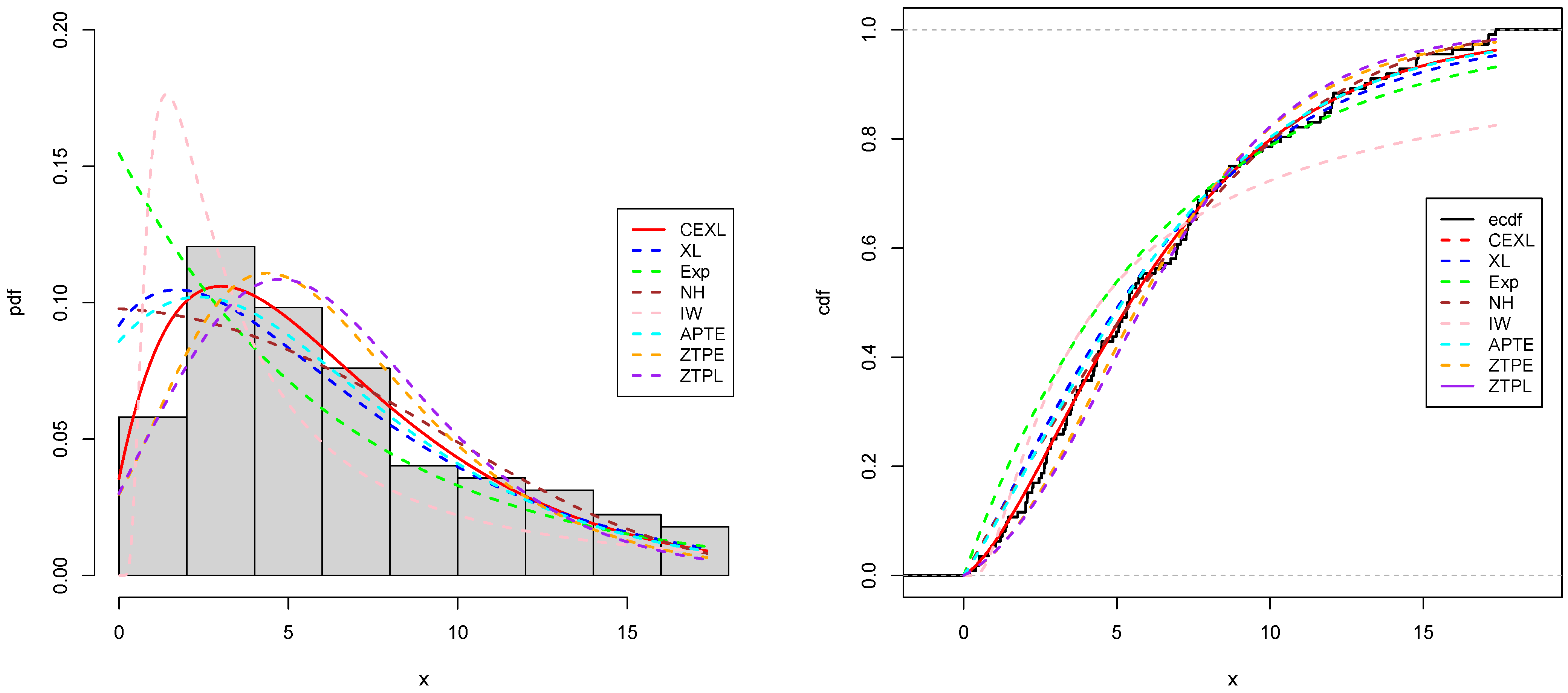
The Inverse Weibull (IW), Nadarajah Haghighi (NH), Alpha power transformed exponential (APTE), Zero truncated Poisson exponential (ZTPE), Zero truncated Poisson Lindley (ZTPL), EXP, and XL distributions are used to compare with our recommended CEXL model. The cdfs of the recommended model can be, respectively, expressed as follows:
Table 13 summarizes the result of the estimation of the unknown parameters for our CEXL model and other selected distributions using the MLE tool. In order to select more adequate model for modelling the two datasets, we compute some statistic measures, notably, Akaike information criterion (
), Bayesian information criterion (
), and Kolmogorov–Smirnov (KS) with its associated
p-values. Also,
Table 13 displays these results. The values of
,
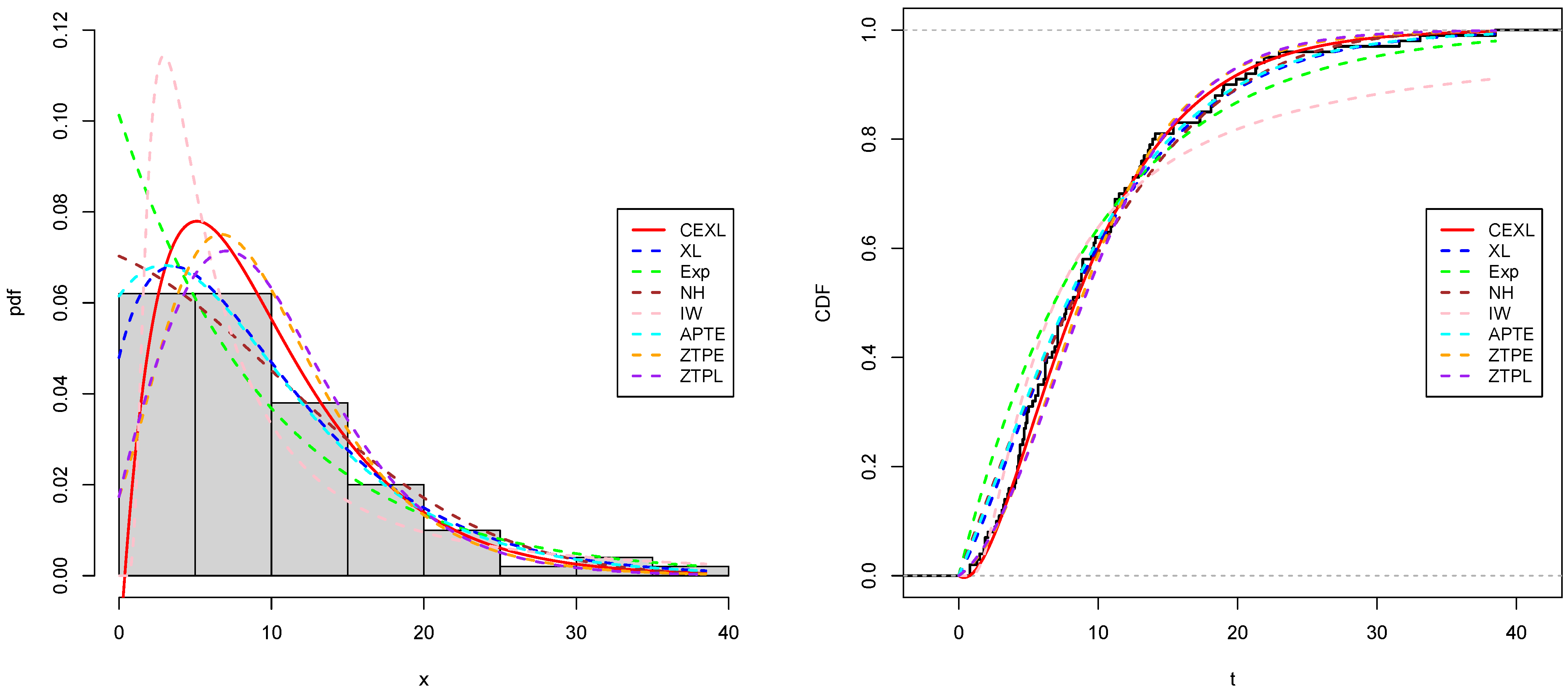
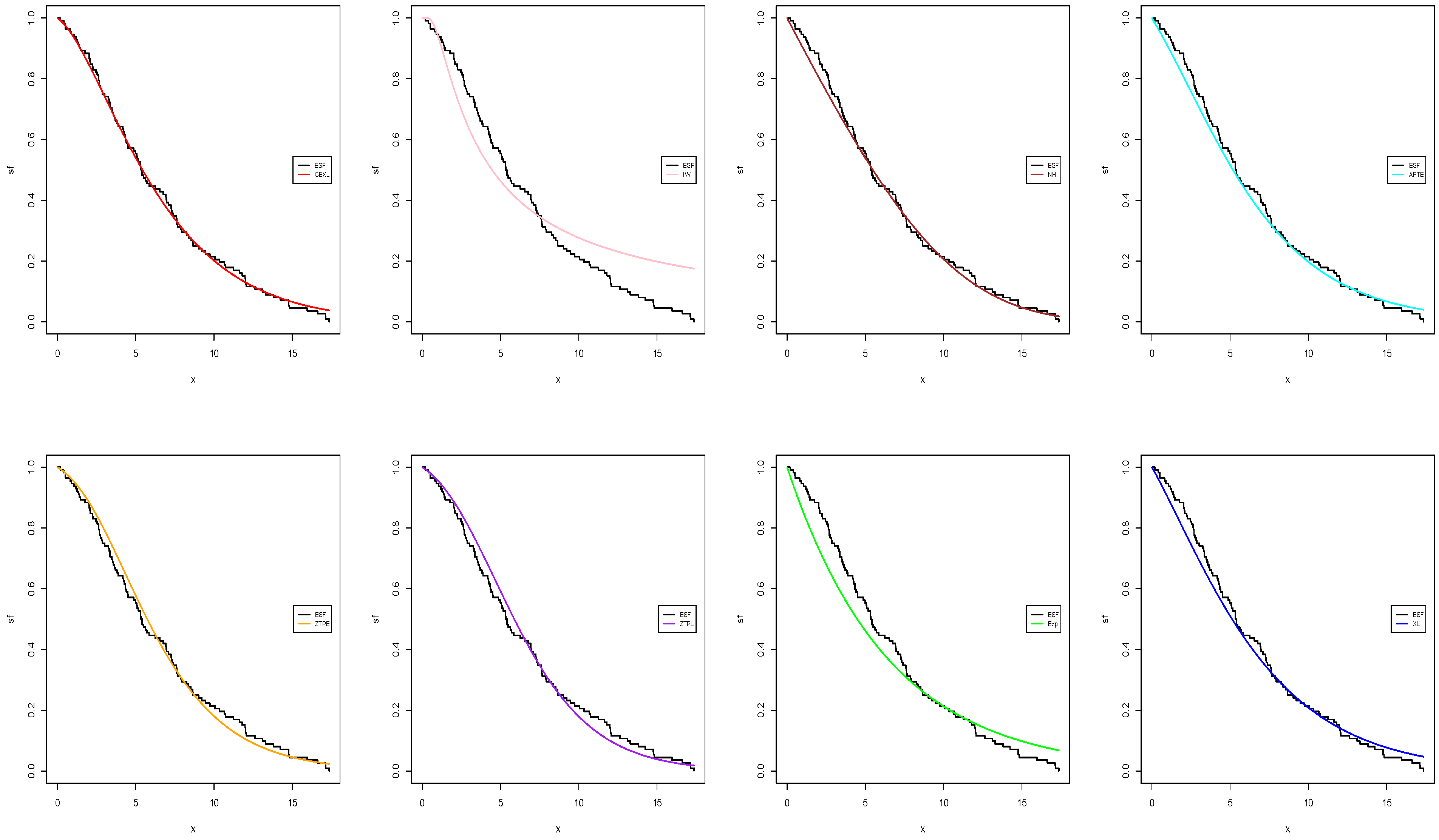
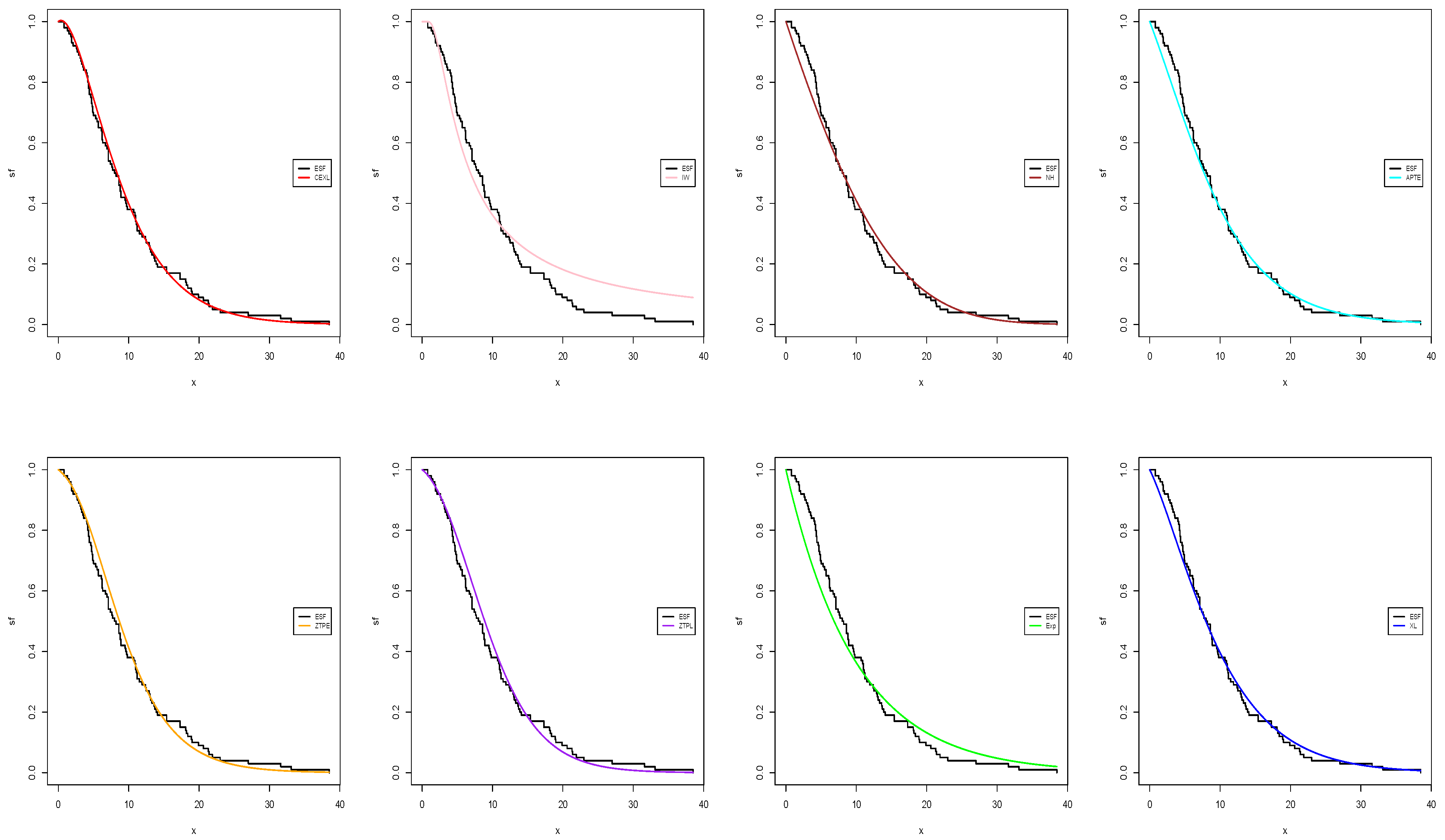
, and KS for our proposed CEXL model are smaller in comparison to the existing well-known distributions, which implies that our CEXL model is best fitting model for analyzing the two datasets than the other fitted distributions.
Figure 6,
Figure 7,
Figure 8 and
Figure 9, respectively, represent the estimated pdf, cdf, and sf for the two datasets using our and the fitting models. These figures also highlight that the CEXL model performed better than the competing models.
Next, we consider the two proposed datasets employing the Bayesian estimation under all suggested loss functions. The obtained results are presented in
Table 14.
7. Conclusions
This study introduces a new lifetime model with two parameters obtained by compounding the exponential and XLindley distributions. Numerous distributional and statistical properties are established. Moreover, the estimation of model parameters is considered by applying two estimation techniques, and for simulation analysis, we perform several experiments for examining the potential of the proposed estimation techniques. It is demonstrated that Bayes under the square error loss function has great efficiency in estimating the unknown parameters among the MLE, LI, and GE methods. Finally, for validation purposes, two real lifetime datasets are applied, and it is shown that our CEXL distribution is the best fitting model compared among other famous competing distributions. For future researches, we may apply several censored samples for estimating the unknown parameters of the CEXL distribution. Also, it is better that to applied this new model environmental and engineering fields.


 ,
, 
