1. Introduction
Quantum Mechanics ushered in an entirely new perspective on nature across all scales. In contrast to the determinism of Classical Mechanics, Quantum Mechanics introduced a probabilistic approach to phenomena on a small scale, effectively accommodating experimental results. While it enabled us to comprehensively describe the quantum realm, it came at the cost of the exact predictability of quantum system evolution. Quantum Field Theory (QFT) subsequently emerged to unify fundamental interactions under a common framework. It quickly became evident that this approach did not readily extend to gravitational interactions due to the probabilistic nature of Quantum Mechanics, in contrast to the deterministic nature of Einstein’s General Relativity (GR), which prohibits non-local interactions.
A theory capable of reconciling the large-scale structure and the Ultraviolet (UV) scale remains elusive. Additionally, neither QFT nor GR can effectively address the Planck scale, where new physics likely comes into play. On the one hand, despite extensive experimental validations, the fundamental meaning of Quantum Mechanics remains elusive. On the other hand, while GR is mathematically rigorous and well-developed, it exhibits inconsistencies at both macro and micro scales [
1]. Efforts to merge the formalisms of GR and QFT have thus far been unsuccessful. Although QFT in curved spacetime offers insights into phenomena at smaller scales (e.g., Hawking Radiation, the Unruh effect, or cosmic inflation), it faces limitations. For instance, GR can be renormalized only to the second loop level, resulting in intractable divergences when applying the same scheme as QFT to gravity [
2]. Furthermore, unlike other fundamental interactions, GR cannot be treated with the Yang–Mills framework due to the absence of a corresponding Hilbert space and a probabilistic interpretation of the gravitational wave function [
3,
4]. Consequently, the quest for a coherent and self-consistent theory of Quantum Gravity remains an active research area.
In recent years, the quantum framework has been adapted to cosmology, where dynamics can be simplified by considering a minisuperspace of variables. This “toy model” has yielded critical insights into the early stages of the Universe. Nonetheless, Quantum Cosmology remains far from being a comprehensive and self-consistent Quantum Gravity theory.
In the context of astrophysics, GR has enjoyed notable success, supported by observations of light deflection, Radar Echo Delay, and precise estimations of Mercury’s perihelion precession. Recent discoveries of gravitational waves and black holes further validate the relativistic description of astrophysical phenomena [
5,
6].
Nonetheless, several shortcomings have emerged in recent years [
7]. For example, GR cannot predict the mass-radius profile of compact objects or the speeds of the farthest stars orbiting galaxies [
8,
9], which have been experimentally measured to be lower than theoretical expectations. To address the latter issue, “Dark Matter”, a hypothetical zero-pressure fluid, was introduced, accounting for 26% of the Universe. However, Dark Matter remains undetected at the fundamental particle level. The cosmological constant
was introduced to explain the observed accelerated expansion of the Universe [
10,
11], referred to as “Dark Energy”, which constitutes approximately 68% of Universe’s energy-matter content. However, at the quantum level, a vast discrepancy exists, with a 120-order magnitude difference between the theoretical and experimental values of
.
In response to these challenges, several new theories have emerged, often beginning with modifications to the Einstein–Hilbert gravitational action, introducing additional curvature invariants [
12] or coupling between geometry and scalar fields [
13,
14,
15]. The simplest extension,
gravity, contains a function of the scalar curvature in the action, resulting in fourth-order field equations [
16,
17,
18,
19,
20,
21]. Certain forms of this theory can solve the Galaxy Rotation Curve problem without invoking Dark Matter, as well as explain the Universe’s exponential expansion without Dark Energy [
22]. Another notable theory is the Starobinsky model [
23], featuring a quadratic term in the scalar curvature and accurately describing cosmic inflation.
Besides
gravity, modifications to GR include non-minimal coupling with one or more dynamical scalar fields. These scalar-tensor theories can be reformulated into higher-order theories via conformal transformations. Furthermore, higher-order curvature invariants, such as the “Gauss–Bonnet” scalar, play a role in modified gravity theories, offering potential solutions to GR’s inconsistencies [
24,
25,
26].
Given the wide range of alternatives to GR, a selection criterion based on Noether symmetries is essential to constrain the starting action [
27,
28,
29]. Testing gravitational theories through observational cosmology serves as an effective approach to identify viable theories with predictive power. Models exhibiting Noether symmetries allow for the selection of Lagrangians with reducible dynamics and conserved quantities, simplifying the study of their dynamical systems and offering physically meaningful models.
In this paper, we study the basic foundations and the applications of modified gravity models containing non-locality in gravitational action. In particular, we start from a general non-local modified action and constrain the functional models by applying the Noether Symmetry Approach. Selected models are thus tested in a cosmological and spherically symmetric background.
The paper is organized as follows: in
Section 2, we summarize the role of non-locality in physics, paying particular attention to gravity theories. In particular, we distinguish between two classes of non-local gravity theories and discuss their features. In
Section 3, the Noether symmetry approach is introduced, as well as how to apply the prescription to gravitational Lagrangians. In
Section 4, we select non-local models by symmetry considerations and find the related cosmological solutions. Moreover, we also analyze the phase space of some selected models and further constrain the functional form of the Lagrangian by searching for fixed points. In
Section 5, we reconstruct the shape of the non-local function by cosmograpic evaluation and compare the results with those obtained in
Section 4. In
Section 6, Noether’s approach is applied to a non-local action in a spherically symmetric background. Again, the resulting model is compared with observations on S2 star orbit. In
Section 7, we search for additional gravitational waves modes by performing the first-order expansion of the metric and, finally, in
Section 8 we conclude the work summarizing the results and discussing the future perspectives.
2. Extensions of General Relativity including Non-Locality
Non-locality is an inherent aspect of Quantum Physics, representing a significant challenge when trying to reconcile the frameworks of QFT and GR. In contrast to classical theories, which are fundamentally local, Quantum Mechanics exhibits a kinematical non-locality. It is crucial to draw a distinction between kinematical and dynamical non-locality. The former pertains to the states that describe a theory, while the latter is related to the interactions within the theory itself. Consequently, dynamical locality (or non-locality) arises from the local (or non-local) form of the action.
2.1. Standard Examples of Non-Locality
In a general context, transcendental functions of fields can be represented using the integral kernels of differential operators. One such operator, denoted as
(where
represents the covariant derivative and
is the metric tensor), plays a role in accounting for long-range non-local effects. This can be expressed in terms of the associated Green function, denoted as
, through the following equation:
In classical theories, at any point during their evolution, the fields can be precisely localized, allowing measurements without disturbing their state. Therefore, classical field theories exhibit what is known as kinematical locality.
Conversely, Quantum Mechanics is inherently non-local. According to Heisenberg’s Uncertainty Principle, it is impossible to precisely localize a given particle. This property implies that a particle, initially at position and moving toward a final position , can follow any conceivable path connecting the two points. Unlike Classical Mechanics, where the actual path between two fixed endpoints is uniquely determined by initial conditions, in Quantum Mechanics all possible paths are simultaneously allowed.
It is essential to note that the kinematical non-locality of the theory does not inherently imply dynamical non-locality. For a theory to exhibit dynamical non-locality, the action itself must possess a non-local form. Another illustration of non-locality in Quantum Mechanics is the phenomenon of entanglement, which results from a kinematical non-locality due to distant interactions between particles.
In the framework of QFT, fundamental interactions display dynamical non-locality when considering their one-loop effective actions. This is evident in cases like the Euler-Heisenberg Lagrangian, as represented by the following equation:
In this equation, represents the electromagnetic tensor, defined via the potential as and . The constants e and m correspond to charge and mass, respectively. The Lagrangian mentioned above is the renormalized one-loop effective Lagrangian that arises after integrating out a massive fermion from the full Lagrangian of quantum electrodynamics. The non-locality here can be attributed to the intrinsic non-local nature of an integration, which can be interpreted as the inverse of a differential operator.
Another example is provided by the low-energy limit of the Yukawa theory, involving a scalar field
with mass
m. The effective Lagrangian is:
The non-locality in this context arises from the operator
and, after performing a Taylor expansion, the Lagrangian can be expressed as:
This formulation turns into the 4-Fermi theory as soon as accounts for the W or Z boson.
2.2. Non-Local Gravity
As mentioned briefly in the introduction, it is worth noting that some of the assumptions made in GR lack direct experimental support. For example, the assumption that the action is linearly dependent on the scalar curvature, giving rise to second-order field equations, is often considered, though no theoretical constraint imposes the action to be linear with respect to R. Additionally, the affine connection is often taken symmetric with respect to the lowest indexes, resulting in a spacetime without torsion. This assumption is rooted in the Equivalence Principle, which is in complete agreement with the Levi–Civita connection. Conversely, in the Einstein–Cartan formalism, the antisymmetric part of the connection is incorporated into the curvature tensor, leading to a description of spacetime that includes both curvature and torsion.
In the large-scale regime, to accommodate the various stages of the universe’s evolution, the cosmological constant was introduced into the action to account for phenomena known as Dark Matter and Dark Energy.
When one relaxes the constraint of having second-order field equations, it becomes possible to extend the Einstein–Hilbert Lagrangian by introducing additional terms involving curvature invariants. One of the most extensively explored extensions is the
gravity, leading to fourth-order field equations that reduce to Einstein ones when
:
Here,
is a general function of the Ricci scalar,
denotes the matter Lagrangian, and
stands for the gravitational coupling, defined as
, where
represents the Newton constant. Additional modified actions can be formulated by incorporating combinations of the Riemann, Ricci, and Weyl tensors. This is the case, e.g., of the so called
Gauss–Bonnet invariant, defined as:
with
and
being the Ricci and the Riemann tensors, respectively. This combination of second-order invariants gives rise to a topological surface term, which in four dimensions is the Euler density. Often, in order to reduce the order of the field equations and the related dynamics, a function of
is evaluated for cosmological and astrophysical purposes [
24,
25].
Another possible modification of GR includes non-local operators into the starting action. The primary distinction when compared to their local counterparts lies in the presence of non-local operators of various forms within the effective action. These operators are intended to bridge the gap between gravitational interactions and the quantum framework.
Depending on the specific nature of non-locality, theories of non-local gravity can be broadly categorized into two primary classes: Infinite Derivative Theories of Gravity (IDGs) and Integral Kernel Theories of Gravity (IKGs).
The former involves analytical transcendental functions of the covariant d’Alembert operator, denoted as □. An illustrative example can be found in the model proposed in Ref. [
30], which offers a solution for classical black holes and Big Bang singularities, as documented in Refs. [
31,
32].
On the other hand, IKGs primarily utilize the inverse operator
. These theories were initially explored in [
33], where it was demonstrated that the application of the non-local operator
to the scalar curvature
R results in the late-time cosmic expansion of the universe without necessitating the inclusion of any Dark Energy contribution. In the pursuit of unifying gravity with other fundamental interactions, IDGs offer renormalizable and unitary quantum gravity theories, as discussed in Ref. [
34]. Conversely, IKGs address infrared (IR) quantum corrections arising from the formulation of QFT in a curved spacetime, as showed in Ref. [
35]. It is worth stressing that, despite these appealing attributes, thus far, no local or non-local theory has emerged that is capable of resolving all the issues associated with large-scale structure and fully aligning with all the currently available observations.
In this paper, we will mostly focus in the latter category of non-local theories, namely, IKGs. They introduce quantum corrections in two distinct regimes through an expansion around
for UV corrections and around
for IR corrections. However, dealing with IR corrections can be challenging for several reasons. First, the Schwinger proper time integral can only be resolved when the masses of matter fields are greater than the potential. Second, in the massless limit, the proper time integration diverges as time progresses. These issues arise from the perturbative approach used for the Schwinger proper time integral, necessitating a non-perturbative technique to capture both UV (
) and IR (
) corrections. The quantum effective action derived from this non-perturbative technique is presented in [
35] as follows:
Here,
represents a generic potential, and
is a surface term defined through the inverse of the d’Alembert operator as:
In this case, the non-locality arises from the integral operator
, which is responsible for the quantum corrections. However, the action (
4) gives rise to non-linear higher-order field equations, potentially complicating the search for exact solutions. As a result, several specific cases have been explored in the literature, one of which is the direct modification of GR presented in [
33]:
In this equation,
is an arbitrary function of the non-local term
. When the action is varied with respect to the metric tensor, it leads to the following field equation:
where the definitions of
are as follows:
In the upcoming sections, we will concentrate on higher-order Integrated Klein–Gordon (IKG) equations, where non-locality is introduced by the operator
. These equations are extensions of the IKGs examined in previous works such as [
33,
36,
37,
38]. While we will not delve into the details of the UV quantum corrections in these theories, it is anticipated that the presence of non-local operators plays a role in achieving renormalizability and unitarity. To seek exact cosmological solutions, we simplify the dynamics by searching for Noether symmetries, an approach developed to identify viable models, as outlined in the next section.
3. The Noether Symmetry Approach
To summarize the essential components of the Noether Symmetry Approach that will be used in
Section 4, we start with the assumption that the Lagrangian remains invariant under certain transformations involving both coordinates
and fields
, i.e.,
Here,
and
represent the infinitesimal generators of the symmetry transformation. The total generator of this transformation is denoted as:
By applying this generator to the Lagrangian and assuming
X to be the generator of a certain symmetry, it can be shown that when the condition
is satisfied; then, the quantity
becomes a first integral of motion [
27]. In this context,
is a general function of coordinates and fields, referred to as a “Gauge Function”. The expression for
(the first prolongation of Noether’s vector) is
This allows us to rewrite the identity in Equation (
12) as:
In cosmological contexts, where the variables are solely time-dependent,
and the identity (
15) become, respectively,
and
For internal symmetries, where the infinitesimal generator
is zero, the condition in Equation (
12) takes the form
By setting
to zero, this equation can be reformulated in terms of the vanishing Lie derivative of the Lagrangian along the flow of the generator
X. Clearly, Equation (
18) leads to introduce a first integral in the Euler–Lagrange equations. This, in turn, enables us to simplify the dynamics and potentially find solutions. In all the scenarios described above, this procedure also aids in discovering physically meaningful models.
4. Non-Local Gravity Cosmology via Noether Symmetries
To illustrate the concepts mentioned above, let us delve into the non-local IKG within the metric framework. This gravitational theory is defined by the following action:
It serves as a straightforward extension of both
gravity and the action (
6). To formulate a Lagrangian suitable for cosmological studies, we introduce an auxiliary local scalar field, denoted as
and defined as:
This definition simplifies the theory into a category of higher-order scalar-tensor models characterized by the action:
In this expression, the constant
is incorporated into the function
F. The action presented in Equation (
21) is a broader form of the one examined in Ref. [
36], where the authors consider the Deser–Woodard action to uncover precise cosmological solutions. From this perspective, the Noether Symmetry Approach offers the advantage of selecting the action based on a physical criterion, out of numerous conceivable choices. Although the Deser–Woodard action is encompassed within Equation (
21), various other models can be chosen through the research for symmetries. Nevertheless, the associated conserved quantities simplify the dynamics and facilitate the identification of analytical solutions. When the cosmological expressions for
R and
are incorporated into a Friedmann–Lemaître–Robertson–Walker (FLRW) spacetime, that is
the action can be recast as:
Here,
and
are Lagrange multipliers,
is the scale factor, and
is the three-dimensional unity matrix. The relation between these two multipliers is found by varying the action concerning
R:
Following a procedure akin to [
36,
39], the constant
can be transformed into a time-dependent scalar field by setting
. Consequently, Equation (
23) can be rewritten as:
When dealing with the Lagrange multipliers method,
and
R must be treated as independent fields so that the variation of the action with respect to the scalar fields
and
leads to the Klein–Gordon equations
Integrating out the second derivatives, the point-like Lagrangian expressed within the configuration space
is:
It is important to note that not all the Euler–Lagrange equations contribute to the dynamics. The equations concerning
and
essentially return the Klein–Gordon equations previously mentioned. The Euler–Lagrange equation involving the scalar curvature provides the cosmological expression for
R by construction. The Euler–Lagrange equation associated with the scale factor, in conjunction with the energy condition, represents the only dynamical equations of motion through which analytical solutions can be derived. These equations correspond to the “0,0” and “1,1” components of the field equations. In the corresponding configuration space, referred to as the minisuperspace, the symmetry generator takes the form:
By applying the Noether symmetry existence condition (
12) to the Lagrangian (
26), we obtain a system of 28 differential equations, six of which are linearly independent [
40]:
A potential solution is given by the following generator:
Additionally, the request for the presence of symmetries also select two functions, namely,
where
represents an arbitrary integration function of
, and
is a function of the scalar curvature, while
,
,
ℓ,
,
n, and
k are constants of integration.
It is worth noting that the second function can be related to the first by choosing an appropriate form for
. Specifically, when
, the second function becomes:
representing a subcase of
. Let us now focus on the function
to explore exact cosmological solutions. For simplicity, we assume that this function is linearly dependent on its argument:
As a result, we obtain:
with
q being a real constant. If we set
, we recover the Starobinsky gravity non-minimally coupled to a scalar field
. The solution of the equations of motion for arbitrary
n yields three different scale factors.
The first one, valid only for
, describes a de Sitter-like expansion:
where we have defined
The second solution arises when the scalar curvature is zero, leading to a power-law scale factor:
In this case, the theory is equivalent to GR when minimally coupled to a scalar field, and the corresponding function is:
Finally, in the last case, we obtain:
In this scenario, the function is constrained with respect to the general one in Equation (
34), resulting in:
It is worth noting that, regardless of the restrictions induced by the Euler–Lagrange equation solutions, the above function remains a generalization of .
The models discussed in this section incorporate higher-order curvature invariants and local scalar fields, potentially capable of inducing both an inflationary phase and late-time cosmic acceleration. The specific behavior depends on the energy regime being considered. A comprehensive analysis is required to determine if these solutions align with cosmological and astrophysical observations. This is just a starting point in the quest to identify reliable non-local gravity models that can address both the UV and IR issues encountered by GR and thereby establish a self-consistent cosmic history.
Comparison with Cosmological Observations
The function in Equation (31) has been studied in Ref. [
41], where the cosmological implications are evaluated, and here the main steps are reported. More precisely, the function studied by the authors can be obtained from Equation (31) by setting
The action can be thus written in terms of the Lagrange multiplier
as
with the definition
The variation of Equation (
42) with respect to the metric and to the scalar field
yield, respectively,
where
is the matter energy-momentum tensor. In a FLRW space-time as in Equation (
22), the field equations become
which, along with the continuity equation
and the two Klein–Gordon equations
form the whole set of cosmological equations. In order to evaluate the dynamics, the order of the above system can be reduced, by means of the following substitutions:
Assuming now a pressureless matter, substituting the form of
in Equation (31) (selected by the imposition of Noether symmetries) and considering the relations (
47), the cosmological equations can be finally written as
with the prime denoting the derivative with respect to
ln(
a), namely, the number of e-folds. Furthermore, in the above equation,
represents the effective EoS parameter
and
the matter density parameter. Once recasting the field equations as a first-order system of ordinary differential equations, the goal is now to search for the critical points and unveiling possible attractors. Specifically, it is possible to study the phase space and to detect the fixed points and the related trajectories around them. The first step is to identify the fixed point, by solving the system for
. To this purpose, we study the cases of cosmological interest, namely, a matter-dominated Universe (
,
), an accelerated Universe (
), and a de Sitter-like Universe (
,
). In
Table 1, the critical points and the corresponding values of
,
, and
are listed.
The first fixed point describes a matter-dominated solution, while the second point cannot describe either accelerated or de Sitter-like solutions since cannot lie within the ranges required for these space-times. The third fixed point corresponds to an accelerated solution when and to a de Sitter Universe fully-dominated by a pure cosmological constant when . In the fourth case, a de Sitter space-time occurs for . Finally, in the fifth case, accelerated solutions occur for and a de Sitter solution for .
Let us now explore the stability of the critical points, examining whether the cosmological solutions previously obtained could potentially act as late-time attractors. To do this, we will compute linear perturbations of the dynamical system and analyze the eigenvalues signs of the Jacobian matrix when calculated for each fixed point. We can distinguish three potential scenarios: if all the real parts of the eigenvalues are negative, we are dealing with a stable (attractor) point. Conversely, if they are all positive, it indicates an unstable (repeller) point. When the signs are mixed, the corresponding critical point is a saddle point.
In order to investigate the stability, let us then consider linear perturbations of the cosmological Equation (
48):
with
being the Jacobian matrix, whose elements are given by
The eigenvalues of
are reported in
Table 2, along with the outcomes of the stability analysis.
Discussing the results of the phase-space analysis, concerning the effective EoS in the non-local model under consideration is of extreme importance in order to establish theoretical constraints for the free parameter
. To accomplish this, it is worth noticing that a Universe devoid of matter and solely featuring a cosmological constant cannot support stable cosmological solutions. The physical solutions detailed in
Table 1, which are derived from the autonomous dynamical system, pertain to critical points within the associated phase space, as pointed out in [
41]. However, they do not offer additional insights into the current matter density value
, as determined by contemporary observations.
Furthermore, it is crucial to make a comparison between the non-local model and the predictions of the ΛCDM model, as well as with scenarios involving dark fluid. While the ΛCDM model has an effective equation of state () equal to , dark fluid scenarios can yield an EoS with .
To make a comparison, let us examine the solutions that were identified for the fourth critical point (refer to
Table 1). In this instance, the condition
imposes the constraint
. However, as previously discussed, the stability of the fourth fixed point narrows this range down to
. Consequently, feasible values for
fall within the confined range
. It is also worth noting that, apart from this issue of fine-tuning, the matter component is entirely absent, rendering it less suitable for cosmological applications.
5. Model Reconstruction via Cosmographic Analysis
In the previous sections, we applied the Noether Symmetry Approach to select the functional form of the action and used the selected non-local function to evaluate the cosmological implications. Here, we consider the general action (
6) again and reconstruct the shape of the distortion function in a model-independent way. Thus, results can be compared with those coming from Noether’s approach in order to check whether the latter is actually capable of selecting viable cosmological theories. The approach presented in this section can be pursued by adopting proper boundary conditions, allowing one to deduce the best analytical approximation of the numerical outcome. More precisely, we initially present the cosmographic method employing Padé polynomials and Bayesian analysis to constrain cosmographic parameters through present data. Next, we explore the dynamic patterns of additional fields resulting from action localization. To these purposes, let us first define
and act a localization process by introducing two auxiliary scalar fields,
U and
V, treated as Lagrange multipliers:
with
Hence, the expressions of the fields
U and
V can be found by varying the above action with respect to
X and
Y, obtaining the two dynamical Klein–Gordon equations
It is important to emphasize that the additional scalars adhere to delayed boundary conditions and become null, along with their initial time derivatives, when assessed at the starting surface. This characteristic guarantees the absence of extra variables, averting the emergence of problematic entities known as ghosts. Furthermore, these auxiliary fields propagate along the characteristic paths of the d’Alembert scalar, aligning the speed of sound with that of light, which mitigates complications often associated with various modified gravity theories. The non-local field Equation (
8), written in terms of the newly introduced quantities, read:
which, in a cosmological background as in Equation (
22), become
with
and
p being the density and the pressure of the fluid, respectively, while
Notice that the three equations are not independent as the third can be obtained as a linear combination of the first two.
The main objective of this section is to offer an alternative understanding of the Universe’s acceleration without encountering the fine-tuning issues associated with the cosmological constant, within the non-local model under consideration. Consequently, we refrain from imposing the
expansion history, or any other specific one, to reduce potential biases in reconstructing
. Instead, our purpose is to ascertain the distortion function in a manner independent of any particular model. To achieve this, we combine analytical and numerical techniques, relying on the following approach. The first step is to consider the Taylor expansion of the scale factor
around the present time
, namely,
which, along with the cosmographic parameters
, can provide the expression of the luminosity distance
in terms of the redshift
, with
In this way, the Hubble parameter can also be recast as
Due to theoretical problems related to the short convergence radius of the Taylor series [
42], the above luminosity distance is often expanded via Padé polinomials, as in Refs. [
43,
44]. Moreover, as pointed out in [
42], the
Padé parametrization stands out as the optimal approximation for yielding precise cosmographic outcomes as it exhibits lower susceptibility to numerical error propagation due to the low number of free parameters. In our case, the
Padé approximation of Equation (
63) yields:
In general, starting from the Taylor expansion,
, the related Padé approximation of the order
is given by
with
and
being defined as:
The values of
, and
can be determined by the Markov chain Monte Carlo (MCMC) analysis based on the Metropolis–Hasting algorithm. Considering the combination of
and
data, at the
confidence level one obtains [
42]:
The above values, along with the expression of the luminosity distance (
63), allow for the precise characterization of the Universe’s evolution up to intermediate redshifts. The first Friedmann equation can be written in terms of the
Padé parametrization of the normalized Hubble rate
, as
. In this regard, let us define, for future convenience, the
Padé parametrization of the normalized Hubble rate
in terms of the e-fold number,
:
where
and where we considered the
Padé approximation of Equation (
67). Also notice that the introduction of the parameter
N makes the time derivative become:
with the prime denoting the derivative with respect to
N.
If we also assume that matter behaves as dust, the second Friedmann equation reads
, with
being the current value of the radiation energy density [
45]. In so doing, the background evolution of the Universe can be then parametrized as
, where
.
In the late times, the contribution of
is negligible, so that
for
. Finally, taking into account Equation (
75) and the cosmological expression of the Ricci scalar, the field Equation (
60); the definitions (
52), (53); and the Klein Gordon Equations (
56) and (57) become, respectively,
Notice that, due to Equation (
61), the fist derivative of
f can be expressed as
, with
. Imposing the retarded boundary conditions
along with
, and
(to avoid divergences of scalar quantities), the system can be solved numerically with respect to
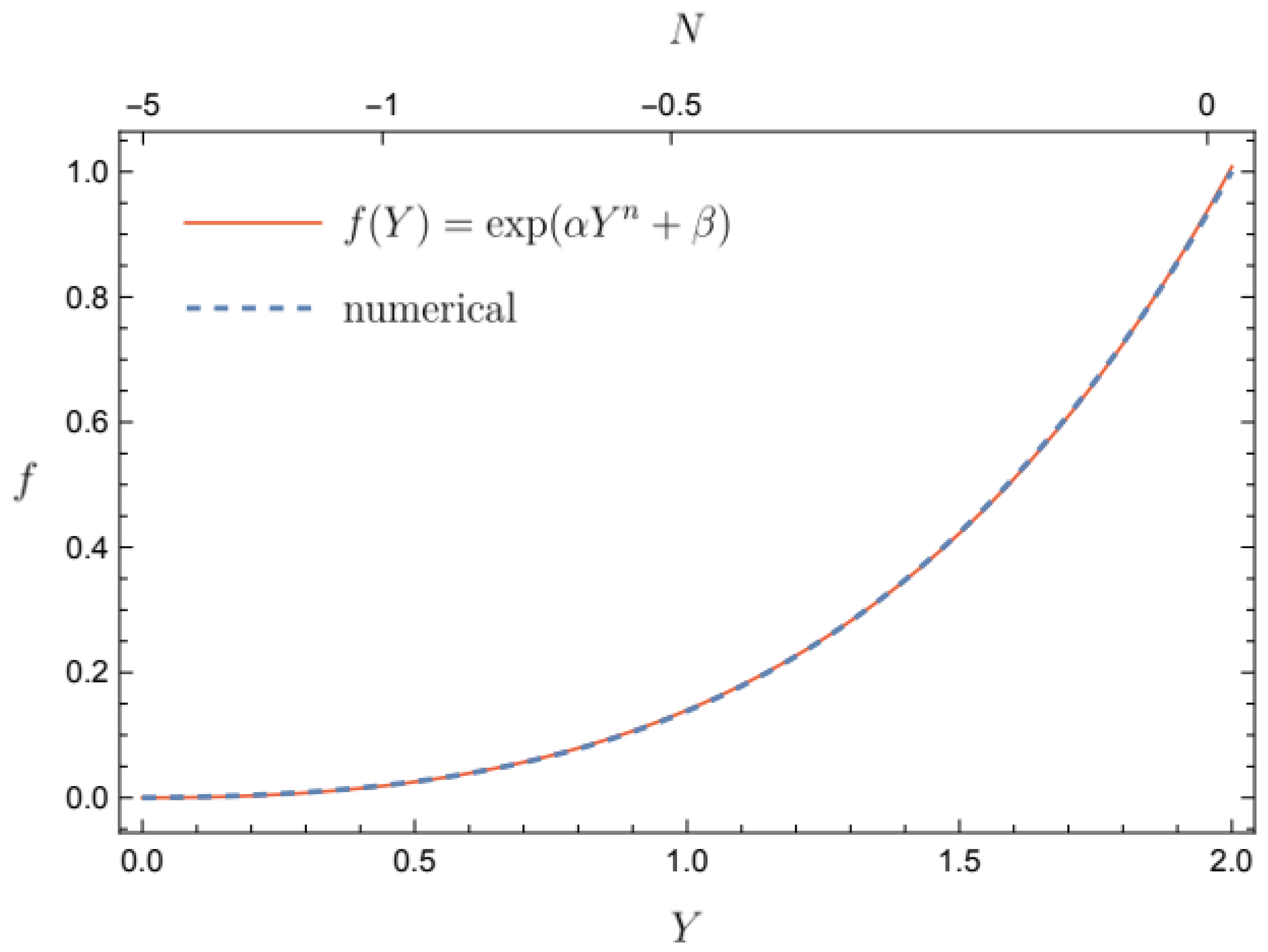
. It turns out that the function
that best fits the numerical solution is:
with
More precisely, the comparison between the numerical solution and the function in Equation (
77) is reported in
Figure 1.
Interestingly, notice that the function selected in this section by cosmographic consideration can be framed within the function in Equation (
30), selected by symmetries. This means that the Noether’s approach is intrinsecally capable of selecting viable function fitting cosmological observations. As we will see in the next section, the same shape of the distorsion function will also be selected by Noether’s approach in spherical symmetry, where will be studied in the weak field limit.
6. Non-Local Gravity in Spherical Symmetry
After exploring the effects of non-local gravity in a cosmological context, now we apply a similar approach to a spherically symmetric spacetime described by the following metric:
To find analytical solutions through the Noether symmetry approach and to derive a set of equations of motion, we consider the spherically symmetric action:
where the auxiliary field
is introduced to localize the dynamics. The configuration space, denoted as
, consists of the variables
since the scalar curvature can be explicitly expressed in terms of the metric potentials
and
. It is important to note that the constraint
cannot be applied
a priori; it arises as a consequence of resolving the field equations, and it is related to the Schwarzschild solution.
The main goal of this section is to demonstrate that the free parameters in the spherically symmetric Lagrangian for a point-like particle, which are determined by the presence of Noether symmetries, can be constrained through astronomical data, specifically data from the S2 star orbiting around SgrA*. These constraints are established within the weak field limit and consider corrections to the Newtonian potential due to non-locality effects.
It is important to stress that the action written above is expressed in terms of the scalar fields
and
using the same localization procedure as in the previous sections. The Klein–Gordon equations for
and
are as follows:
whereas variations with respect to the metric yield the field equations:
Before deriving the point-like Lagrangian, it is worth noting that the metric depends on both the radial coordinate
r and the time coordinate
t. Therefore, the infinitesimal generator
consists of two components, namely,
and
. After considering the form of the d’Alembert operator in spherical symmetry and integrating out the second derivatives, the canonical Lagrangian is given by:
and the corresponding symmetry generator is
Applying Noether’s Theorem to the point-like Lagrangian (
84), we identify two models as follows:
To explore the weak-field limit, we narrow down the range of solutions to a particular subclass where the Birkhoff theorem holds, which means that both
and
are time-independent. This assumption is quite reasonable as an initial approximation, given that in the weak-field limit, a static and spherically symmetric spacetime adequately describes the dynamics around SgrA*. In light of this, let us recast the line element as:
Our goal is to investigate the Post-Newtonian limit of the theory, aiming to constrain the non-local action based on observations from the S2 star’s orbit around SgrA*. To achieve this, we perform an expansion of the metric components. We expand the
component up to the sixth order and the
component up to the fourth, resulting in:
These expansions yield the following expressions:
In the above expressions,
and
represent the Newtonian potentials derived from the expansion of
and
, respectively, and
and
are constants. Setting
,
and taking into account the function in Equation (
87), the Klein–Gordon equations along with the field equations give rise to the following system:
where the derivative with respect to
r is denoted by a prime. We can express the solutions to the above system in terms of the effective gravitational constant,
, with
representing a real constant. Substituting the perturbations from Equation (
90) into the system, we obtain:
The lengths scales
and
are related to the scalar fields
and
, which in turn are connected to the concept of non-locality. Before considering the experimental observations of the S2 star’s orbit, we must further constrain the free parameters
. This can be achieved by examining the second-order expansion of the potential
, i.e.,
by means of which we deduce that the constant
must be set to 1, thus recovering the Newtonian potential as a specific limit. The other two free parameters,
and
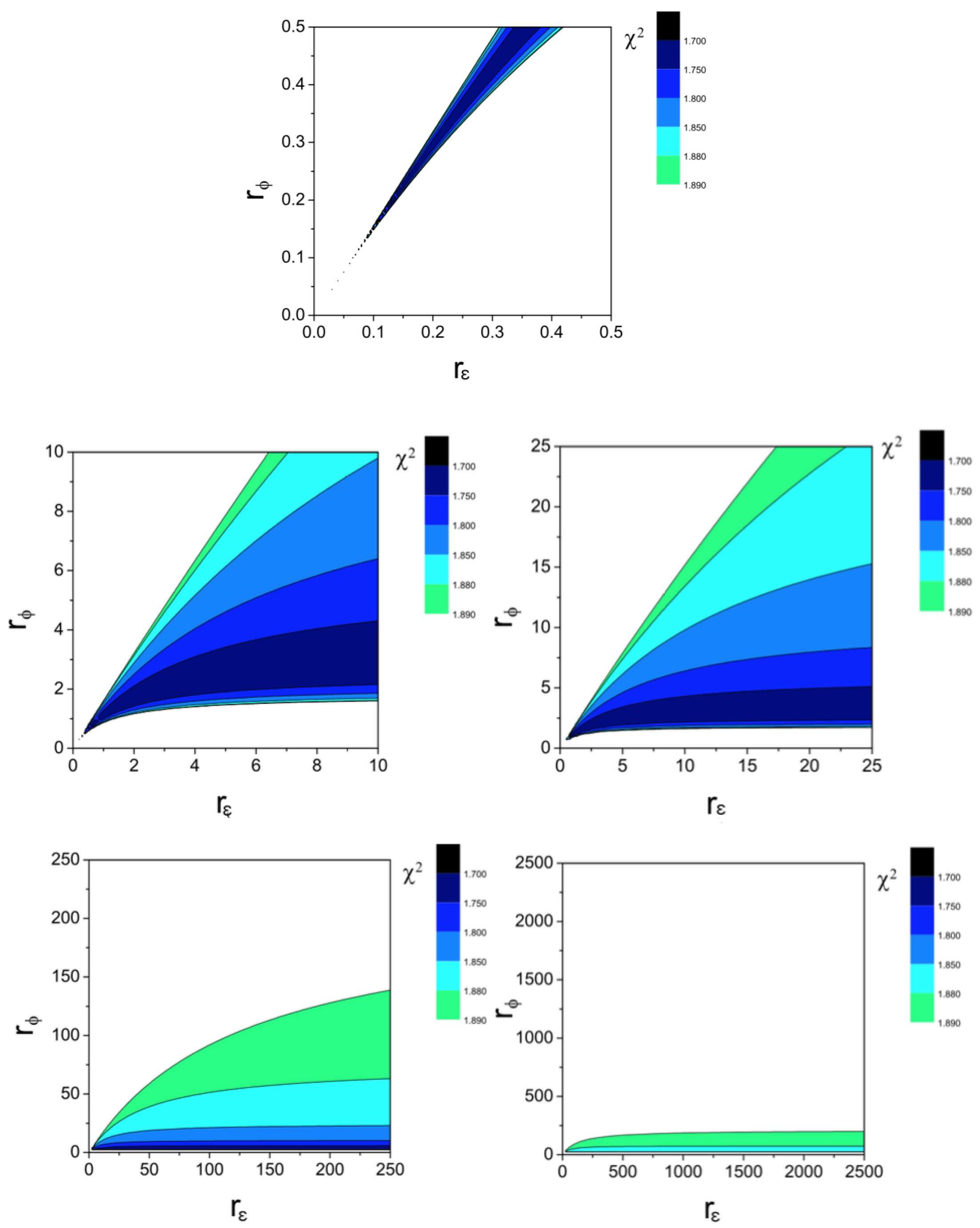
, can be constrained using a two-body simulation of S2 orbiting around SgrA*. Let us define the reduced mass
as
, where
M represents the mass of SgrA*, and
is the mass of S2. According to the data available in Ref. [
46], we vary the values of
and
to identify solutions that yield a lower
compared to the Keplerian orbit (where
). Following the approach of Refs. [
47,
48], we calculate the reduced
as follows:
where (
) and (
,
) represent the observed and theoretical apparent positions, respectively.
N is the number of observations,
is the number of initial conditions, and
and
denote the uncertainties of the observed positions. The graphs in
Figure 2 depict the
values in different regions of the parameter space
.
From these graphs, it is evident that the optimal value for lies within the range 0.1–2.5 AU. However, the analysis of the reduced primarily constrains the length as is related to the non-dynamical scalar field , which serves as a mathematical tool for localization purposes.
To determine the potential energy in the weak-field limit, we can use the expansion of the potential
, leading to the following expressions
which allows us to calculate the energy as:
This equation incorporates non-local corrections related to the function
, which enables us to calculate the precession per orbital period (see
Figure 3).
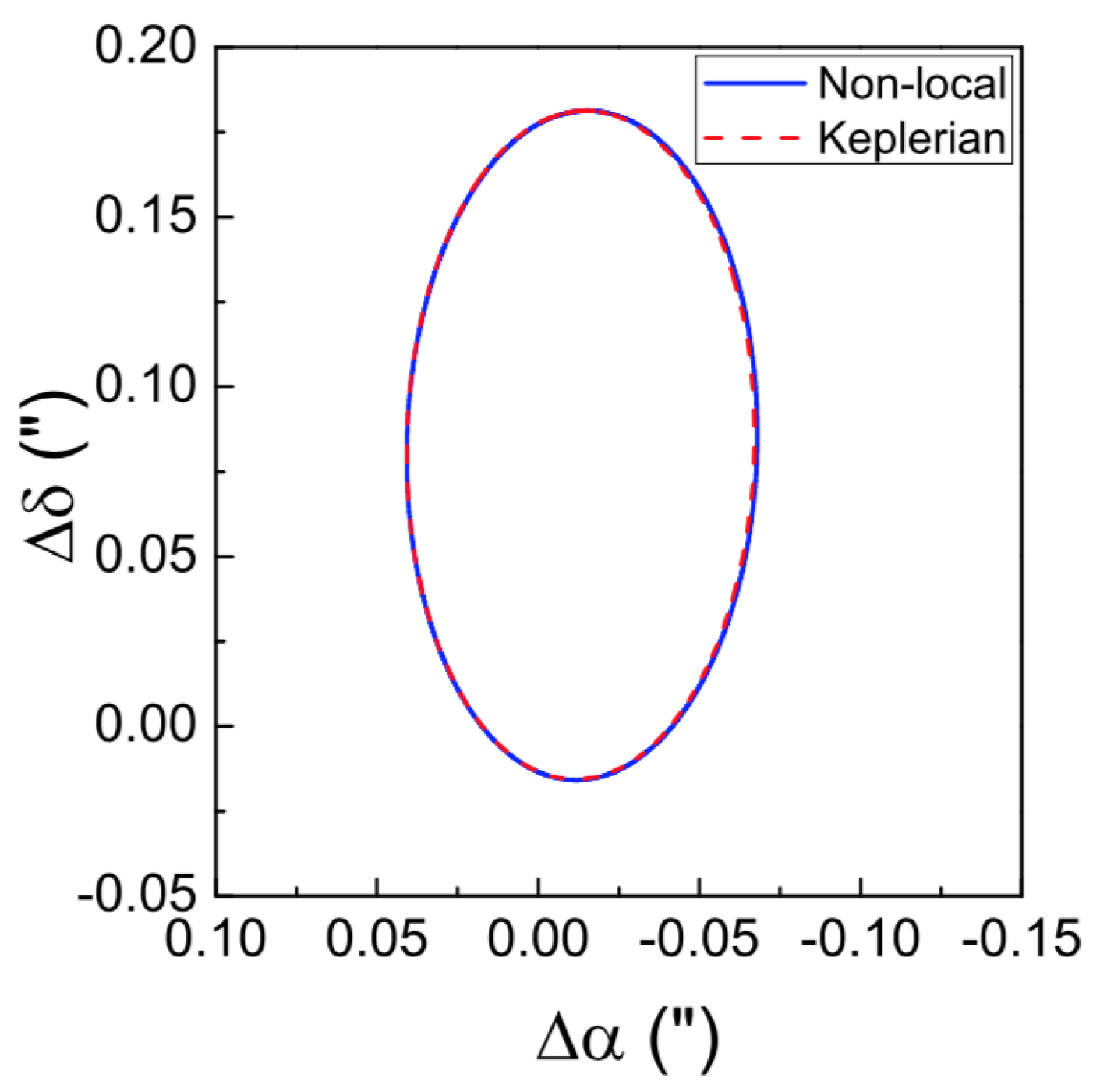
In conclusion, by considering the values
AU and
AU, corresponding to a
of approximately 1.72, the comparison between the Keplerian orbit of the S2 star and the non-local orbit is illustrated in
Figure 4 and
Figure 5.
These figures demonstrate that certain regions align with observations even more closely than the Keplerian model. This selection of the non-local action is fine-tuned to make the scalar degrees of freedom,
and
, match astrometric data. The results highlight that corrections from non-local gravity effects can be compared with data, presenting a method for fitting astrophysical scales to reveal potential non-local effects. As a final remark, we want to point out that, when the non-local term is not present in the starting action, the weak-field analysis provides a Yukawa-like potential for the resulting
-like model, in addition to the standard Newtonian potential. This is clearly shown in [
49], where the authors also study the orbits in
gravity and the perihelion precession of different planets in a Yukawa-like potential.
7. Gravitational Waves
Let us finally consider the function in Equation (
34) and set
,
, and
, in order to study the presence of additional modes in the gravitational waves. To this purpose, we plug a first-order expansion of the metric, namely,
into the non-local field equations and obtain [
50,
51]
where
is the zero-order matter energy-momentum tensor and
. In vacuum and in the k-space, the trace of the above equation becomes:
with
being the Fourier transformation of the metric perturbation
. Using the inverse Fourier transformation of
, i.e.,
we obtain
where
is a suitable complex function and
are the m-frequencies
with
being the solutions of the linear equation
In order to investigate the polarizations and oscillation patterns of waves described by Equation (
100), we employ the geodesic deviation equation for a wave propagating along the
-direction within a local proper reference frame
. The tensor
is the so called “electric” component of the Riemann tensor and can be written as a tensor function of
as
By substituting the relation
and the form of
(
100) into Equation (
104), one obtains a system of three differential equations whose solution provides the polarization modes of the gravitational waves. Keeping
k fixed, setting
and
, we obtain:
The solutions correspond to the two polarization modes of GR, namely, the plus and cross polarizations. These modes are linked to the purely transverse, massless nature of 2-helicity waves linked to the frequency
. On the other hand, it is also possible to obtain other polarization modes by considering
,
, which is equal to the square of
m-th mass of scalar field (where
). In this case, the system reads
By integrating the above system, one obtains
further mixed massive scalar modes, both transverse and longitudinal, with zero-helicity. The perturbation
can be thus written as
with
and
being the standard polarization modes of GR, that is,
and with
admitting four polarization modes of the form
Three out of six modes, however, are negligible with respect to the others when the gravitational wave speed approach c, namely, when the mass of the non-local gravitational wave goes to zero, as pointed out in Ref. [
52]. Therefore, only three modes survive, namely, two massless 2-helicity tensor modes and one massive 0-helicity scalar mode, exactly like
gravity.
Let us conclude by pointing out that identifying additional modes, such as the scalar mode derived in this context, serves as a significant indicator to distinguish and resolve the ambiguities in modified gravity theories at a fundamental level.
8. Conclusions
In this work, we investigated various aspects of non-locality, with a primary focus on non-local theories of gravity. More specifically, we explored three distinct categories of IKG theories and identified the corresponding actions using the Noether Symmetry Approach. In
Section 4, we delved into a specific action depending on the scalar curvature and containing the non-locality through the function
. The presence of symmetries enabled us to discover exact cosmological solutions that naturally account for accelerated cosmic expansion, all without the need for fine-tuning parameters. It is important to note that the models selected through these symmetries align with criteria related to unitarity and super-renormalizability in certain effective theories of quantum gravity (see [
31,
32,
53,
54] for further details). This observation suggests that the Noether Symmetry Approach might serve as a criterion for selecting physically viable theories.
From this perspective, a prospective avenue for cosmological purposes within non-local gravity theories involves constraining free parameters through observational data. An example in this direction is detailed in Ref. [
55].
Subsequently, after simplifying the action to a dual-scalar tensor theory, with a scalar field non-minimally coupled to gravity, we derived the field equations in a FLRW-like universe.
To explore the cosmic dynamics, we employed dimensionless parameters and reformulated the cosmological equations as a self-contained set of differential equations that dictate the behavior of the effective EoS. Then, we examined the solutions within this system, taking into account the non-local contributions introduced by the exponential function , which naturally arise from Lagrangian symmetries. We then conducted a phase-space analysis, identifying critical points and assessing their stability. By studying linear perturbations of the dynamical system and the eigenvalues of the Jacobian matrix at each fixed point, we sought to identify unstable points, saddle points, and attractor solutions in the late-time context. Particularly intriguing were the solutions corresponding to a matter-dominated universe and an accelerated universe, which act as cosmological attractors if and , respectively. Notably, for , we obtain a de Sitter universe characterized by dominance of the cosmological constant, with the associated fixed point being a stable attractor.
Consequently, we studied the physical implications of the non-local scenario in comparison to the ΛCDM and dark fluid models. To further corroborate the viability of the model under consideration, it would be valuable to conduct a direct comparison with cosmological observations through a numerical analysis employing Bayesian methods. This approach could place constraints on the parameter and provide a comprehensive understanding of cosmic evolution.
The incorporation of non-local terms in the gravitational Lagrangian offers a natural means to regulate the transition from a matter-dominated phase to a late accelerated expansion, potentially addressing cosmological tensions and other recent observational challenges.
Then, we explored a minimal non-local extension of GR in spherical symmetry and again applied the Noether symmetry prescription to constrain the resulting model using astrometric data from the S2 star orbit. The analysis involves adjusting the length scales to minimize the reduced until it better matches experimental observations than traditional Keplerian orbits. This development is significant because it highlights the feasibility of directly investigating non-local effects through galactic-scale observations.
Another result of this work reveals the existence of a scalar gravitational mode, alongside the conventional massless tensor modes, within a non-local gravity theory selected by Noether symmetries. This theoretical framework can be viewed as a straightforward expansion of GR, incorporating non-local corrections. The additional scalar mode emerges when we examine plane waves, assuming the observer is positioned at a considerable distance from the wave source.


