Abstract
Large-scale symmetric and asymmetric matrices have emerged in predicting the relationship between genes and diseases. The emergence of large-scale matrices increases the computational complexity of the problem. Therefore, using low-rank matrices instead of original symmetric and asymmetric matrices can greatly reduce computational complexity. In this paper, we propose an approximation conjugate gradient method for solving the low-rank matrix recovery problem, i.e., the low-rank matrix is obtained to replace the original symmetric and asymmetric matrices such that the approximation error is the smallest. The conjugate gradient search direction is given through matrix addition and matrix multiplication. The new conjugate gradient update parameter is given by the F-norm of matrix and the trace inner product of matrices. The conjugate gradient generated by the algorithm avoids SVD decomposition. The backtracking linear search is used so that the approximation conjugate gradient direction is computed only once, which ensures that the objective function decreases monotonically. The global convergence and local superlinear convergence of the algorithm are given. The numerical results are reported and show the effectiveness of the algorithm.
Keywords:
approximation conjugate gradient method; low-rank matrix recovery; backtracking linear search technique; global convergence; superlinear convergence MSC:
49M37; 65K05; 90C30; 90C56
1. Introduction
Problem Description Motivation
The low-rank matrix plays an important role in a broad range of applications and multiple scientific fields. For example, many bioinformatics experts use the matrix restoration technique to predict the relationship between diseases and genes [1]. In many bioinformatics problems, the information between genes and diseases is presented in the form of a symmetric or asymmetric matrix, but the dimensions of symmetric and asymmetric matrices are extremely large, which makes it difficult to calculate effectively in practical situations and even leads to the inability to perform calculations. Hence, it is often possible to recover it due to the low-rank structure. In many cases, the rank r of the low-rank matrix is fixed and the matrix decomposition is completed, where is a known matrix and is the variable matrices of the following problem:
In many cases, matrix M is a symmetric matrix, i.e., and the matrix decomposition , , problem (1) is equivalent to solving the following low-rank symmetric matrix recovery problem:
As the factorized problem (1) or (2) involves only or variables, these methods are, in general, more scalable and can cope with larger matrices. The solution to the matrix recovery problem has also attracted the interest of many scholars.
On the Euclidean manifold, Sun and Luo [2] established a theoretical guarantee for the factorization-based formulation to correctly recover the underlying low-rank matrix. Tu et al. [3] proposed a Procrustes Flow algorithm for solving the problem of recovering a low-rank matrix from linear measurements.
On other Riemannian manifolds, Keshavan et al. [4] introduced an efficient algorithm such that the method could reconstruct matrix from . Ngo and Saad [5] described gradient methods based on a scaled metric for low-rank matrix completion. Vandereycken [6] proposed a new algorithm for matrix completion. Mishra and Sepulchre [7] introduced a nonlinear conjugate gradient method for solving low-rank matrix completion. Mishra et al. [8] proposed a gradient descent and trust-region algorithm for low-rank matrix completion. Boumal and Absil [9] exploited the geometry of the low-rank constraint to recast the problem as an unconstrained optimization problem on a single Grassmann manifold. Wei et al. [10] introduced a family of Riemannian optimization algorithms for low-rank matrix recovery problems. In the past year, Najafi and Hajarian [11] proposed an improved Riemannian conjugate gradient method to solve robust matrix completion problems. Duan et al. [12] proposed the Riemannian conjugate gradient method for solving the low-rank tensor completion problem.
In addition to the aforementioned work, there are also some algorithms for solving matrix completion problems (see [13,14,15,16,17,18]). For solving matrix recovery problems, some algorithms and related research have also been widely studied (see [19,20,21,22,23,24]).
Inspired by the algorithm ideas in [25,26], this paper proposes an approximation conjugate gradient method to solve the low-rank matrix recovery problem. The approximation conjugate gradient direction is given such that the search direction is the descent direction of the objective . The algorithm avoids the singular value decomposition of the matrix and only obtains the search direction of the problem through the multiplication of the matrix. The backtracking line search technique ensures that the objective function of problem (1) is monotonic descent.
In this paper, the approximation conjugate gradient direction is introduced in Section 2. In Section 3, the detailed steps of the approximation conjugate gradient algorithm are proposed. The global convergence of the algorithm is given in Section 4. In Section 5, the local superlinear convergence of the algorithm is given. Numerical results are presented in Section 6, and in Section 7, some conclusions are given.
Notation
In this paper, the low-rank matrix recovery problem is solved by the approximation Newton algorithm. In problem (1), let denote the variables, and be the optimal solution of objective function . The F-norm of matrix Z is defined as . A symmetric and positive semidefinite matrix is represented as . Given any matrix , denotes the usual trace inner product of A and B.
2. The Approximation Conjugate Gradient Step
In this paper, we propose a new approximation conjugate gradient algorithm for solving problem (1). Next, we first introduce the traditional conjugate gradient algorithm for solving the unconstrained nonlinear programming problem.
In the Euclidean case, the conjugate gradient methods are line search algorithms to solve the unconstrained nonlinear programming problem, where the objective function is . The sequence in is generated by
with for all from an initial point , and the search directions are computed using the gradient as and
for all . The computation of real values is crucial for the performance of conjugate gradient methods. A famous real value of is
It was proposed by Fletcher [27].
To solve problem (1), we let
Hence,
and
on iteration point .
The sequence is generated by
from an initial point with for all . The search direction are computed using the gradient as and
for all . To obtain better search directions, we constructed the following real value of Algorithm 1 based on the structure of the problem itself,
where denotes the usual trace inner product of and .
| Algorithm 1 (ACGA) |
Input: Choose an initial , where , . Let , and set . Main step: 1. If , then compute and let . 2. If and , then stop, is the optimal solution of problem (1). 3. Compute such that
4. Let . 5. Calculate , if , then stop, is the optimal solution of problem (1). 6. Compute as (2) and
let , go to 3. |
3. The Approximation Conjugate Gradient Algorithm (ACGA)
In Section 2, we introduce the approximation conjugate gradient step with updated real value .
Remark 1.
We obtain the step size by the backtracking line search based on objective function , i.e., given , let until (5) holds.
Remark 2.
We can randomly generate initial matrix and initial matrix with rank r. We can generate the matrices and as follow,
4. Convergence Analysis
In this section, to prove the convergence of the algorithm (ACGA), we require the model to satisfy the following assumption:
Assumption 1.
Assume that the objective functions of problem (1) are twice continuous differentiable, i.e., for any , it is twice continuous differentiable. For any point in our method, we define the level set
Assume the level set is bounded.
Assumption 2.
Assume the gradient of is Lipschitz-continuous, i.e., there exists such that
for any .
The bounded function is important for the proof of convergence of Algorithm 1 and the following lemma presents the boundedness of the objective function .
Lemma 1.
Under Assumption 1, there exists constant and such that
Proof.
The proof is similar to Lemma 3.2 in [28]. □
The purpose of step 3 of Algorithm 1 is to monotonically decrease the objective function of problem (1). Hence, we need to prove that when Algorithm 1 does not terminate.
Lemma 2.
If Algorithm 1 dose not terminate, i.e., for constant , we have , then
Proof.
If Algorithm 1 dose not terminate, i.e., , then according to the definition of , we have that
If , by (4) and (6), we have that
If , then we have that
□
Step 3 is important for Algorithm 1 because it ensures that the objective function is monotonically decreasing. But we must prove that step 3 is to terminate in a finite step, i.e., there exists such that (5) holds.
Lemma 3.
Under Assumptions 1 and 2, let be the sequence generated by Algorithm 1, then step 3 is to terminate in a finite step, i.e., there exists such that (5) holds.
Proof.
Suppose Algorithm 1 dose not terminate on iteration k, i.e., there exists positive constant such that . First, we prove that is bounded for all . We use mathematical induction to prove this conclusion. When , we have , according to Lemma 1, we have , suppose is bounded, then by (3), we have that
By (4), if , then
Hence, let , we have that . Hence, by (7), we have that
According to the assumption of the bounded of , we obtain that there exists a positive constant such that
According to Assumption 2, the gradient of is Lipschitz-continuous, then
By (9), we want , then
By (10), we have that
Hence, we let , then the conclusion holds.
If , similar to the proof of (9), we have that
Hence, to ensure , we want , then
which means that
Let , then the conclusion holds. □
The following theorem shows that the sequence generated by Algorithm 1 converges to the critical point of problem (1).
Theorem 1.
Under Assumptions 1 and 2, the sequence generated by Algorithm 1 satisfy
It means that the iteration sequence converges to the critical point of problem (1).
5. Local Convergence
In Section 4, we have shown that the sequence generated by the conjugate gradient algorithm converges globally to zero. We now discuss the superlinear convergence in a neighborhood of the solution .
First, we show that if , then for any iteration index k.
Lemma 4.
Under Assumptions 1 and 2, let be the sequence generated by Algorithm 1, if , then .
Proof.
First, we consider the follow inequality
We want , then
By (16) and , we have that holds, which means that . □
Finally, we show that the sequence generated by Algorithm 1 converges to critical point superlinearly.
Theorem 2.
Under Assumptions 1 and 2, if and the objective function satisfies the local error bound condition, i.e., there exists such that for all , then the sequence generated by Algorithm 1 converges to critical point superlinearly.
Proof.
Because , according to Lemma 4, we have . Then,
According to Assumption 2,
Since , we know that
for large enough k.
Divide by on both sides of the inequality (21), we have that
As and when , we can obtain that
as , i.e.,
which means that the sequence generated by Algorithm 1 converges to critical point superlinearly. □
6. Numerical Results
In Section 3, the approximation conjugate gradient method is given, and the global and local superlinear convergence of this algorithm are given in Section 4 and Section 5, respectively. Next, we give the numerical experiments to illustrate the performance of the method proposed in this paper. We apply ACGA to synthetic problems. The synthetic data of the experiments are increased as they are in [29]. First, the matrices and with independent and identically distributed Gaussian entries such that is filled with zero-mean and unite-variance nonindependent Gaussian entries are given. Then, the sample is given at random, where is the oversampling factor. To test the effectiveness of the algorithm, we compare ACGA to RMC [29], AOPMC [30], GRASTA [31], and method RTRMC [9].
RMC was the method for solving the low-rank matrix completion, in which the fraction of the entries was corrupted by non-Gaussian noise and typically outliers. This method smoothed the norm, and the low-rank constraint was dealt with by Riemannian optimization.
AOPMC was a robust method for recovering the low-rank matrix using the adaptive outlier pursuit technique and Riemannian trust-region method when part of the measurements was damaged by outliers.
GRASTA was a Grassmannian robust adaptive subspace tracking algorithm. This method needed the rank-r SVD decomposition for the matrix and could improve computation speed while still allowing for accurate subspace learning.
RTRMC exploited the geometry of the low-rank constraint to recast the problem as an unconstrained optimization problem on a single Grassmann manifold. The second-order Riemannian trust-region methods and Riemannian conjugate gradient methods are used to solve the unconstrained optimization problem.
Before solving the low-rank recovery problem, we will introduce the parameters selected in the actual calculation of the algorithm proposed in this paper. The important parameter of this paper is . To obtain a larger search step size and the objective function of problem descent more quickly, the backtracking line search parameter in step 3 of the algorithm selects a smaller value close to 0, so is selected in the algorithm proposed in this paper.
To solve the low-rank recovery problem using the algorithm in this paper, we use MATLAB (2014a) to write a computer program, and the computer is a ThinkPad T480 (CPU is i7-8550U, main frequency is 1.99 Hz, memory is 8 G). The termination accuracy of the algorithm is chosen by , and , respectively.
In this paper, we selected 12 problems to test the effectiveness of the algorithm. The number of rows and columns of the selected questions, as well as the rank of matrices U and V, are shown in the following Table 1. In Table 1, m and n denote the number of rows and columns of matrix M, respectively. r denotes the rank of matrices U and V. To test our algorithm, we randomly generated 50 different scenarios for each problem in Table 1 and obtained the final number of iterations by a weighted average of all random problem results. We have set three different termination accuracies for our algorithm () and used our algorithm to calculate the test problems in Table 1 for each accuracy. We also used the four classic methods mentioned above to solve every test problem in Table 1 and recorded the number of iterations of each method to solve every test problem in Table 1. The comparison results of our algorithm with the other four algorithms under different termination accuracies are shown in Figure 1, Figure 2 and Figure 3.

Table 1.
The information of test problems.
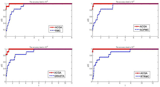
Figure 1.
Comparison results of the number of iterations between ACGC and the other four algo−rithms when and .
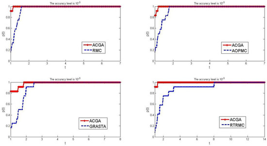
Figure 2.
Comparison results of the number of iterations between ACGC and other four algorithms when and .
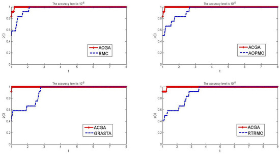
Figure 3.
Comparison results of the number of iterations between ACGC and other four algorithms when and .
To draw a comparison diagram of the results of five algorithms, we use the performance comparison formula of the algorithm proposed by Dolan and More [32] to calculate the computational efficiency between different algorithms. Here are the specific formulas:
where S denotes the set of algorithms. Let P denote problems set, and . For , let
where represent the efficiency of each solver.
We solve the test problems in Table 1 using ACGA, RMC, AOPMC, GRASTA and method RTRMC, respectively. First, the terminate parameter is chosen by . The test results are reported in the following Figure 1.
From Figure 1, we can see that our algorithm has significant effectiveness compared to the other four algorithms for calculating low-rank matrices. Especially when , our algorithm has reached 0.83 and even reached 0.9 in comparison with RTRMC, but other algorithms only reach between 0.1 and 0.2. This indicates that at an accuracy level of , our algorithm can solve 83–90% of test problems faster than the other four algorithms. By (23) and (24), the red curve representing our algorithm tends to 1 faster than the blue curve representing other algorithms, indicating that our algorithm is more effective in solving the test problems in Table 1 using all five algorithms. From the abscissa of the four subgraphs mentioned above, it can be seen that our algorithm spends much fewer iterations solving most testing problems than the other four algorithms. In summary, our algorithm is more effective in solving the test problems in Table 1.
Next, we use five algorithms to solve the test problems when the terminate parameter is chosen by . The test results are reported in Figure 2.
From Figure 2, we can see that when the termination parameter is set to , it indicates that our algorithm’s red curve tends to 1 much faster than the other four algorithms. When , the red curve has already reached 0.8, or even 0.9, while other algorithms only reach around 0.2, with a worst-case value of 0.1. This indicates that even with improved termination accuracy, our algorithm still has high computational efficiency, i.e., our algorithm spends fewer total iterations when solving more than of problems. According to the abscissa of each subgraph, it can be seen that our algorithm spends much fewer iterations in solving many testing problems in Table 1 than the other four algorithms, indicating that our algorithm has higher efficiency in solving testing problems.
From Figure 3, we clearly see that with the continuous improvement of termination accuracy, the five algorithms listed in this article have shown a decrease in efficiency when solving test problems compared to those with accuracies of and . In other words, the number of iterations required to solve all test problems has greatly increased. However, when the termination accuracy is , our algorithm still has higher efficiency compared to the other four algorithms. The main manifestation is that the red curve representing our algorithm has reached a range of 0.8 to 0.9 when , but other algorithms only reach around 0.4 or 0.5. This indicates that our algorithm spends less iteration time solving most test problems than the other four algorithms. In addition, the speed at which the red curve tends to 1 is also faster than the blue curve representing other algorithms, and it can be clearly seen from the abscissa that although the overall solving efficiency has decreased, our algorithm still spends far fewer iterations on solving some problems than the other four algorithms.
Finally, we changed the termination parameter to and still used five different algorithms to solve the test problem. The results are reported in Figure 3.
We choose the rank and for solving the test problems in Table 1 using Algorithm 3, RMC, AOPMC, GRASTA and RTRMC, respectively. The number of iterations of every method for solving every problem of Table 1 is reported. Using (23) and (24), we obtain a comparison graph of the number of iterations when we solve every problem in Table 1 using four algorithms. The comparison results are reported in Figure 4.
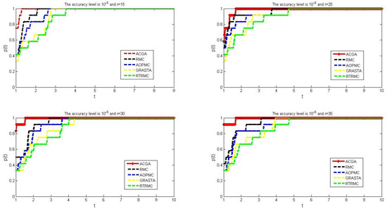
Figure 4.
Comparison results of the number of iterations for five algorithms when we choose , , , and , respectively.
By (23) and (24), we can see that the red curve tends to 1 and is also faster than other curves representing other algorithms. This means that our algorithm costs fewer iterations than the other four algorithms when we solve all test problems in the table, with , and , respectively.
Next, we will test our algorithm on the Netflix dataset, which is a real-world dataset in the Netflix Prize [33]. Netflix is a movie rental company that recommends movies to its users. Hence, they have much information from users. This information is translated into a matrix (this matrix is denoted as M). To test our algorithm, we randomly selected 10 matrices of in M, and the rank of U and V are chosen by . We will choose and to test five algorithms. The number of iterations for each algorithm at different accuracies and ranks is recorded in Figure 5.
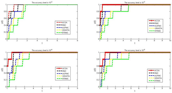
Figure 5.
Comparison results of number of iterations for five algorithms when we choose , and , respectively.
From Figure 5, we can see that the speed at which the red curve tends towards 1 is the fastest at different accuracies. This means that for different termination accuracies, the number of iterations of our algorithm is less than the other four algorithms in most cases when solving all real-test problems, indicating that our algorithm is effective in solving practical problems.
We determine the complexity of the algorithm by recording the time when the algorithm solves the problems in Table 1. In other words, the more time is spent, the higher its complexity; conversely, the lower its computational complexity. Next, we calculate the test problems in Table 1 using five different algorithms and record the time by each algorithm in Figure 6.
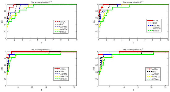
Figure 6.
Comparison results of time for five algorithms when we choose , and , respectively.
From Figure 6, we can see that the speed at which the red curve tends towards 1 is the fastest, indicating that our algorithm spends less time than other algorithms when solving most of the test problems in Table 1. In particular, from Figure 6, we can see that the yellow curve representing the SVD decomposition algorithm is much lower than the red curve representing our algorithm, which means that our algorithm has a lower computational complexity than the SVD algorithm.
7. Concluding Remarks
The main purpose of this paper is to introduce the approximation conjugate gradient method, which avoids the complex SVD decomposition for solving the low-rank matrix recovery. The idea is to extend the approximation conjugate gradient method and the conjugate gradient parameter update technique to the matrix calculation and obtain the search direction. The backtracking linear search technique ensures the global convergence of the algorithm. At the same time, this technique ensures that the objective function decreases monotonously. The local superlinear convergence of the algorithm is also given, and the numerical results are reported to show the effectiveness of the algorithm.
Author Contributions
Methodology, P.W. and D.Z.; validation, Z.C.; formal analysis, Z.C. and P.W.; writing original draft preparation, Z.C.; writing review and editing, P.W. and Z.C.; visualization, Z.C. and P.W.; supervision, P.W. and D.Z. All authors have read and agreed to the published version of the manuscript.
Funding
This research was funded by National Natural Science Foundation (11371253) and Hainan Natural Science Foundation (120MS029).
Data Availability Statement
Data are contained within the article.
Conflicts of Interest
The authors declare no conflict of interest.
References
- Xu, J.; Zhu, W.; Cai, L.; Liao, B.; Meng, Y.; Xiang, J.; Yuan, D.; Tian, G.; Ynag, J. LRMCMDA: Predicting miRNA-diease association by interating low-rank matrix completion with miRNA and disease similarity information. IEEE Access 2020, 8, 80728–80738. [Google Scholar] [CrossRef]
- Sun, R.; Luo, Z. Guaranteed matrix completion via non-convex factorization. IEEE Trans. Inf. Theory 2016, 62, 6535–6579. [Google Scholar] [CrossRef]
- Tu, S.; Boczar, R.; Simchowitz, M.; Soltanolkotabi, M.; Recht, B. Low-rank solutions of linear matrix equations via procrustes flow. In Proceedings of the International Conference on Machine Learning, PMLR, New York City, NY, USA, 19–24 June 2016; pp. 964–973. [Google Scholar]
- Keshavan, R.H.; Montanari, A.; Oh, S. Matrix completion from a few entries. IEEE Trans. Inf. Theory 2010, 56, 2980–2998. [Google Scholar] [CrossRef]
- Ngo, T.; Saad, Y. Scaled gradients on grassmann manifolds for matrix completion. In Proceedings of the Advances in Neural Information Processing Systems, Lake Tahoe, NV, USA, 3–6 December 2012; pp. 1412–1420. [Google Scholar]
- Vandereycken, B. Low-rank matrix completion by Riemannian optimization. SIAM J. Optim. 2013, 23, 1214–1236. [Google Scholar] [CrossRef]
- Mishra, B.; Sepulchre, R. R3MC: A Riemannian three-factor algorithm for low-rank matrix completion. In Proceedings of the 53rd IEEE Conference on Decision and Control, Los Angeles, CA, USA, 15–17 December 2014; pp. 1137–1142. [Google Scholar]
- Mishra, B.; Meyer, G.; Bonnabel, S.; Sepulchre, R. Fixed-rank matrix factorizations and Riemannian low-rank optimization. Comput. Stat. 2014, 29, 591–621. [Google Scholar]
- Boumal, N.; Absil, P. Low-rank matrix completion via preconditioned optimization on the grassmann manifold. Linear Algebra Appl. 2015, 475, 200–239. [Google Scholar]
- Wei, K.; Cai, J.; Chan, T.; Leung, S. Guarantees of Riemannian optimization for low rank matrix recovery. SIAM J. Matrix Anal. Appl. 2016, 37, 1198–1222. [Google Scholar] [CrossRef]
- Najafi, S.; Hajarian, M. An improved Riemannian conjugate gradient method and its application to robust matrix completion. Numer. Algorithms 2023, 1–14. [Google Scholar] [CrossRef]
- Duan, S.; Duan, X.; Li, C.; Li, J. Riemannian conjugate gradient method for low-rank tensor completion. Adv. Comput. Math. 2023, 49, 41. [Google Scholar] [CrossRef]
- Wen, Z.; Yin, W.; Zhang, Y. Solving a low-rank factorization model for matrix completion by a nonlinear successive over-relaxation algorithm. Math. Prog. Comput. 2012, 4, 333–361. [Google Scholar]
- Hardt, M. Understanding alternating minimization for matrix completion. In Proceedings of the 2014 IEEE 55th Annual Symposium on Foundations of Computer Science, Philadelphia, PA, USA, 18–21 October 2014; pp. 651–660. [Google Scholar]
- Jain, P.; Netrapalli, P. Fast exact matrix completion with finite samples. In Proceedings of the 28th Conference on Learning Theory, Paris, France, 3–6 July 2015; pp. 1007–1034. [Google Scholar]
- Yi, X.; Park, D.; Chen, Y.; Caramanis, C. Fast algorithms for robust PCA via gradient descent. In Proceedings of the 30th International Conference on Neural Information Processing Systems, Barcelona, Spain, 5–10 December 2016; pp. 4159–4167. [Google Scholar]
- Zheng, Q.; Lafferty, J. Convergence analysis for rectangular matrix completion using burer-monteiro factorization and gradient descent. arXiv 2016, arXiv:1605.07051. [Google Scholar]
- Chen, J.; Liu, D.; Li, X. Nonconvex rectangular matrix completion via gradient descent without l2∞ regularization. IEEE Trans. Inf. Theory 2020, 66, 5806–5841. [Google Scholar]
- Haldar, J.P.; Hernando, D. Rank-constrained solutions to linear matrix equations using powerfactorization. IEEE Signal Process. Lett. 2009, 16, 584–587. [Google Scholar] [CrossRef] [PubMed]
- Ma, C.; Wang, K.; Chi, Y.; Chen, Y. Implicit regularization in nonconvex statistical estimation: Gradient descent converges linearly for phase retrieval, matrix completion and blind deconvolution. Found. Comput. Math. 2019, 20, 451–632. [Google Scholar]
- Ma, C.; Li, Y.; Chi, Y. Beyond procrustes: Balancing-free gradient descent for asymmetric low-rank matrix sensing. IEEE Trans. Signal Process. 2021, 69, 867–877. [Google Scholar]
- Tong, T.; Ma, C.; Chi, Y. Accelerating ill-conditioned low-rank matrix estimation via scaled gradient descent. J. Mach. Learn. Res. 2021, 22, 1–63. [Google Scholar]
- Zilber, P.; Nadler, B. GNMR: A provable one-line algorithm for low rank matrix recovery. SIAM J. Math. Data Sci. 2022, 4, 909–934. [Google Scholar]
- Li, H.; Peng, Z.; Pan, C.; Zhao, D. Fast Gradient Method for Low-Rank Matrix Estimation. J. Sci. Comput. 2023, 96, 41. [Google Scholar] [CrossRef]
- Upadhyay, B.B.; Pandey, R.K.; Liao, S. Newton’s method for intervalvalued multiobjective optimization problem. J. Ind. Manag. Optim. 2024, 20, 1633–1661. [Google Scholar] [CrossRef]
- Upadhyay, B.B.; Pandey, R.K.; Pan, J.; Zeng, S. Quasi-Newton algorithms for solving interval-valued multiobjective optimization problems by using their certain equivalence. J. Comput. Appl. Math. 2024, 438, 115550. [Google Scholar]
- Fletcher, R. Practical Methods of Optimization; John Wiley & Sons: New York, NY, USA, 2013. [Google Scholar]
- Zhang, H.; Conn, A.R.; Scheinberg, K. A derivative-free algorithm for least-squares minimization. SIAM J. Optim. 2010, 20, 3555–3576. [Google Scholar] [CrossRef]
- Cambier, L.; Absil, P.-A. Roubst low-rank matrix completion by riemannian optimization. SIAM J. Sci. Comput. 2016, 38, S440–S460. [Google Scholar] [CrossRef]
- Yan, M.; Yang, Y.; Osher, S. Exact low-rank matrix completion from sparsely corrupted entries via adaptive outlier pursuit. J. Sci. Comput. 2013, 56, 433–449. [Google Scholar] [CrossRef]
- He, J.; Balzano, L.; Szlam, A. Incremental gradient on the Grassmannian for online foreground and background separation in subsampled video. In Proceedings of the 2012 IEEE Conference on Computer Vision and Pattern Recognition (CVPR), Providence, RI, USA, 16–21 June 2012; pp. 1568–1575. [Google Scholar]
- Dolan, E.D.; More, J.J. Benchmarking optimization software with performance profiles. Math. Profiles 2002, 91, 201–213. [Google Scholar] [CrossRef]
- Bennett, J.; Lanning, S. The Netflix Prize. In Proceedings of the KDD Cup and Workshop, San Jose, CA, USA, 12 August 2007; p. 35. [Google Scholar]
Disclaimer/Publisher’s Note: The statements, opinions and data contained in all publications are solely those of the individual author(s) and contributor(s) and not of MDPI and/or the editor(s). MDPI and/or the editor(s) disclaim responsibility for any injury to people or property resulting from any ideas, methods, instructions or products referred to in the content. |
© 2024 by the authors. Licensee MDPI, Basel, Switzerland. This article is an open access article distributed under the terms and conditions of the Creative Commons Attribution (CC BY) license (https://creativecommons.org/licenses/by/4.0/).