Nonlinear Dynamics of a New Class of Micro-Electromechanical Oscillators—Open Problems

Abstract

In this paper, we propose a new class of micro-electromechanical oscillators. Some investigations based on Melnikov’s approach are applied for identifying some chaotic possibilities. We demonstrate also some specialized modules for investigating the dynamics of these oscillators. This will be included as an integral part of a planned much more general Web-based application for scientific computing. It turns out that the theoretical apparatus for studying the circuit implementation (design, fabricating, etc.) of the considered differential model for large parameter values is extremely complex and requires a serious investigation. This is the reason to offer this model to the attention of specialists working in this scientific direction. Some open problems related to the use of existing computer algebraic systems for the study of this class of oscillators for large values of $n,m$ and N are also posed. In general, the entire article is subordinated to this frank conversation with the readers with the sole purpose being the professional upgrading of the specialized modules provided for this purpose in subsequent licensed versions of CAS.

1. Introduction

The micro-electromechanical oscillators are important apparatus that have a large usage in many different real life fields which need very fine clock synchronization. We can mention the telecommunications, video transfers, GPS systems, the work of all microprocessors and many others. This wide applicability leads to a necessity of further investigations of their theoretical foundations as well as the possible implementation in the practice.

A variety of micro-electromechanical oscillators is governed by a version of the Mathieu equation that harbors both linear and cubic nonlinear time-varying stiffness terms—the subharmonic resonance is investigated in [1]; the possible chaotic behavior generated by such models is studied in [2], etc. An application of the oscillator dynamics to the filtering problem is provided in [3]. The time-varying capacitors are included in the study of [4] to investigate the nonlinear dynamics of a micro-electromechanical system. A comprehensive study devoted on the topic can be found in [5].

Various results related to hetero/homoclinic bifurcation, optimal control in the nonlinear dynamics, higher-order Melnikov analysis of homo/hetero clinic bifurcation in mechanical oscillators, and bifurcation and chaos in a single d.o.f. mechanical system can be found in [6,7,8,9,10,11,12,13].

In [14], the authors study the dynamics of a class of hypothetical micro-electromechanical oscillator of the form

$$\left\{\begin{array}{ccc}{\displaystyle \frac{dx}{dt}}\hfill & =& y\hfill \\ {\displaystyle \frac{dy}{dt}}\hfill & =& bx-{\displaystyle \sum _{i=0}^{\left[\frac{n}{2}\right]-1}}{b}_i{x}^{n-2i}-ϵ\left(\alpha y+(1+cos\left(\omega t\right))\left(ax+{\displaystyle \sum _{i=0}^{\left[\frac{m}{2}\right]-1}}{a}_i{x}^{m-2i}\right)\right).\hfill \end{array}\right.$$

(1)

In the present article, we suggest a new trigonometric class of micro-electromechanical oscillators and study their dynamics. The first important task we investigate is the possible chaotic behavior of our model. Here, we use the method proposed by Melnikov in [15]. It gives us an analytic tool for establishing the existence of transfer homoclinic points of the Poincare map for a periodic orbit of a perturbed dynamical system. Some analytical conditions are obtained. Also, the effects of all free parameters in the planar differential system are analyzed.

Our second task is to consider the performance these new models produce. Several simulations are composed, and the generated results are discussed in the light of the theoretical and practical significance they lead. We demonstrate also some specialized modules for investigating the dynamics of these hypothetical oscillators. The derived results can be used as an integral part of a much more general application for scientific computing—for some details, see [14,16,17,18]. Other dynamic models can be found in [19,20,21,22,23,24,25,26].

Last but not least, some open problems related to the use of existing computer algebraic systems for the study of this class of oscillators for large values of $n,m$ and N are also posed.

In the proposed article (for the first time), “friendly fire” is directed at the thousand-strong army of collaborators (full-time and voluntary) of companies creating CAS and Web-based applications (with paid or free access) for scientific computing.

The plan of the paper is as follows. We state our model in Section 2. Our results in the light of Melnikov’s approach can be found in Section 3. Some open problems are discussed in Section 4. Some simulations are presented in Section 5. An alternative to control the chaotic behavior under probability distributed parameters $a_i$, $i=0,1,\dots ,\left[\frac{m}{2}\right]$, $b_i$, $i=0,1,\dots ,\left[\frac{n}{2}\right]$, $g_j$, $j=1,2,\dots ,N$ is given in Section 5.1. A special case is considered in Section 6. In Section 7, we will focus on some difficulties the user encounters when using Computer Algebraic Systems for scientific computing. We conclude in Section 8.

2. The Model

We consider the following new class of micro-electromechanical oscillators

$$\left\{\begin{array}{ccc}{\displaystyle \frac{dx}{dt}}\hfill & =& y\hfill \\ {\displaystyle \frac{dy}{dt}}\hfill & =& bx-{\displaystyle \sum _{i=0}^{\left[\frac{n}{2}\right]-1}}{b}_i{x}^{n-2i}-ϵ\left(\alpha y+{\displaystyle \sum _{j=1}^N}{g}_{j}sin\left(j\omega t\right)\left(ax+{\displaystyle \sum _{i=0}^{\left[\frac{m}{2}\right]-1}}{a}_i{x}^{m-2i}\right)\right),\hfill \end{array}\right.$$

(2)

where $0\le ϵ<1$, n and m are odd, N is an integer, and the coefficients a, b, $\alpha$, $a_i$, $i=0,1,\dots ,\left[\frac{m}{2}\right]$, $b_i$, $i=0,1,\dots ,\left[\frac{n}{2}\right]$, $g_j$, $j=1,2,\dots ,N$ are real numbers.

Let us consider, for example, the case $n=m=3$. We can fix without community restriction b and $b_0$ at $b=b_0=1$. For $ϵ=0$, the resulting Hamiltonian of the system (2) is

$$H(x,y)=\frac{1}{2}{y}^2-\frac{1}{2}{x}^2+\frac{1}{4}{x}^4.$$

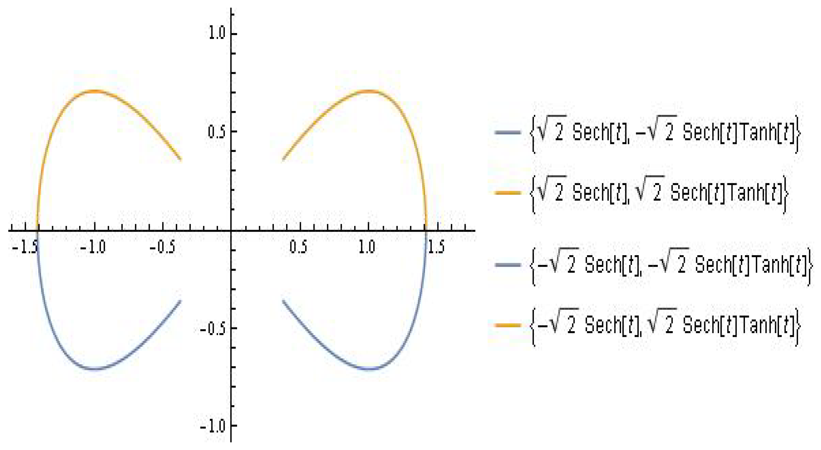
There is a saddle point at the origin, centers at $(\pm 1,0)$, and a double homoclinic orbit given by (see Figure 1)

$$\begin{array}{c}{x}_0\left(t\right)=\pm \sqrt{2}secht\hfill \\ y_0\left(t\right)=\mp \sqrt{2}sechttanht.\hfill \end{array}$$

(3)

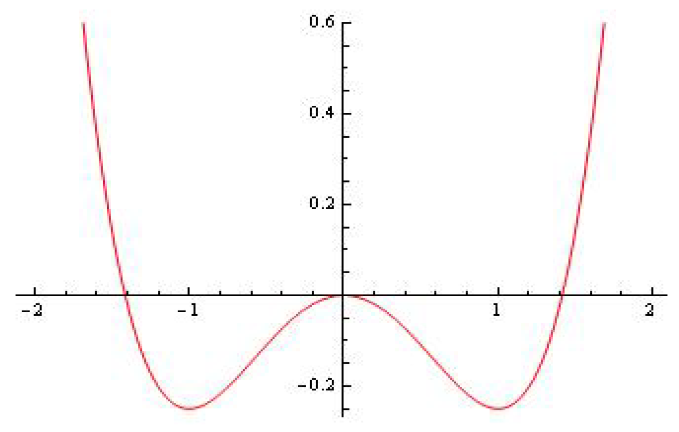
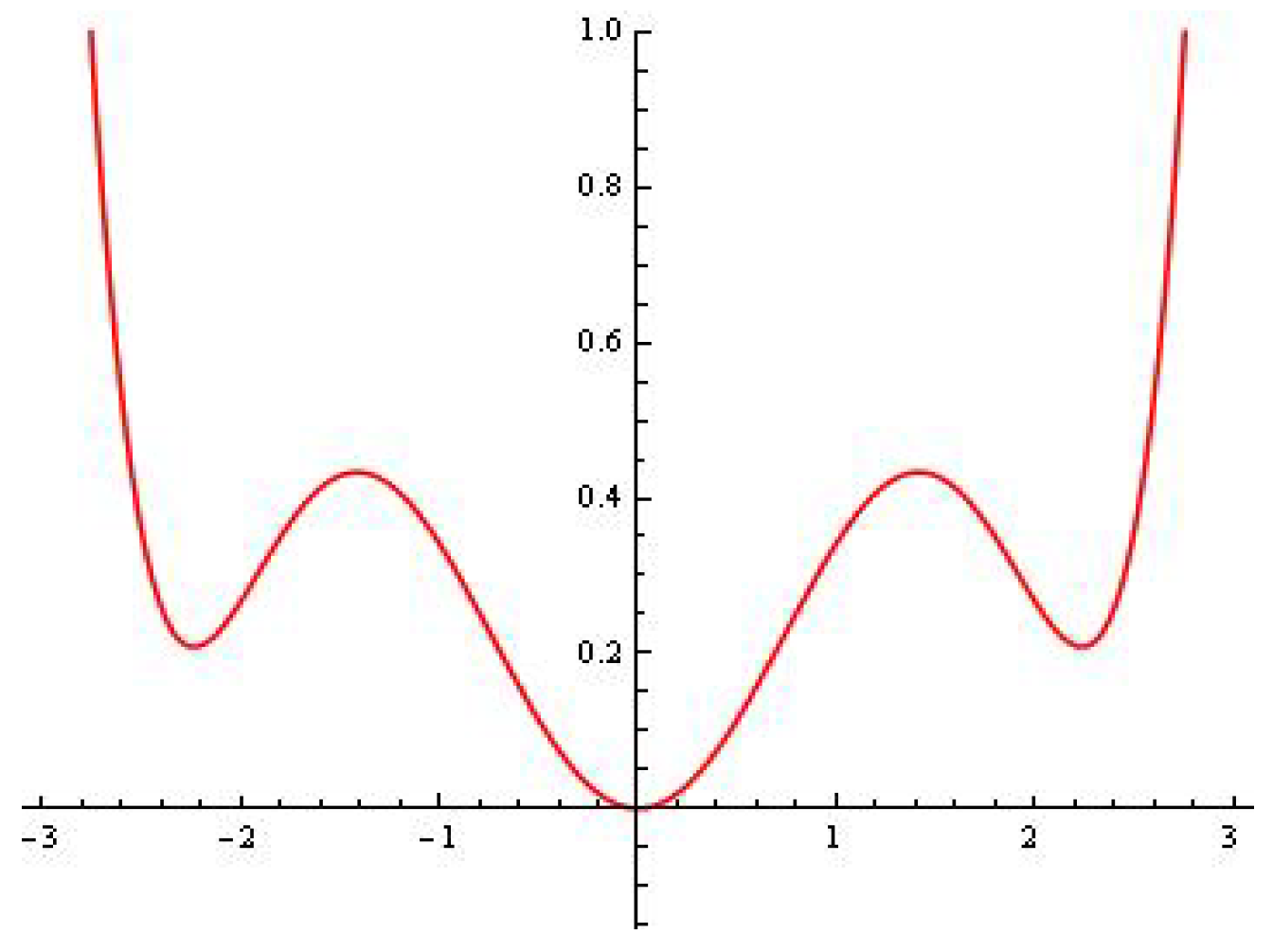
We refer to [14,27,28,29,30] for more details. The potential energy $V\left(x\right)=-\frac{1}{2}{x}^2+\frac{1}{4}{x}^4$ is shown in Figure 2.

3. Results in the Light of the Melnikov’s Approach

The Melnikov function gives a measure of the leading order distance between the stable and unstable manifolds when $ϵ\ne 0$ and can be used to tell where the stable and unstable manifolds intersect transversely. By definition, the homoclinic integral of Melnikov is given by

$$M\left(t_0\right)={\displaystyle {\int }_{-\infty }^{\infty }}{y}_0\left(t\right)\left(\alpha y_0\left(t\right)+{\displaystyle \sum _{j=1}^N}{g}_{i}sin\left(j\omega (t+t_0)\right)\left(a{x}_0\left(t\right)+{\displaystyle \sum _{i=0}^{\left[\frac{m}{2}\right]-1}}{a}_i{x}_0^{m-2}\left(t\right)\right)\right)dt,$$

(4)

where the functions $x_0\left(t\right)$ and $y_0\left(t\right)$ are defined by Equation (3). From a numerical point of view, the task of finding a root of $M\left(t_0\right)$ is more interesting given that the parameters appearing in the proposed differential model are subject to a number of restrictions of a physical and practical nature.

3.1. The Case $n=m=3$ and $N=1$

Suppose that $n=m=3$ and $N=1$. We compute the integral of Melnikov replacing formulas (3) in Equation (4):

$$\begin{array}{ccc}M\left(t_0\right)\hfill & =& {\displaystyle {\int }_{-\infty }^{\infty }}{y}_0\left(t\right)\left(\alpha y_0\left(t\right)+g_{1}sin\left(\omega (t+t_0)\right)\left(a{x}_0\left(t\right)+a_0{x}_0^3\left(t\right)\right)\right)dt\hfill \\ \hfill & =& {\displaystyle {\int }_{-\infty }^{\infty }}(-\sqrt{2}sechttanht)\left(\alpha (-\sqrt{2}sechttanht)+\right.\hfill \\ \hfill & & \left.+g_{1}sin\left(\omega (t+t_0)\right)\left(a\sqrt{2}secht)+a_0{\left(\sqrt{2}secht\right)}^3\right)\right)dt\hfill \\ \hfill & =& \frac{4}{3}\alpha -\frac{1}{6}{g}_1\pi {\omega }^2(6a+a_0(4+{\omega }^2))csch\left(\frac{\pi \omega }{2}\right)cos\left(t_0\omega \right),\hfill \end{array}$$

(5)

Thus, we obtain the following statement.

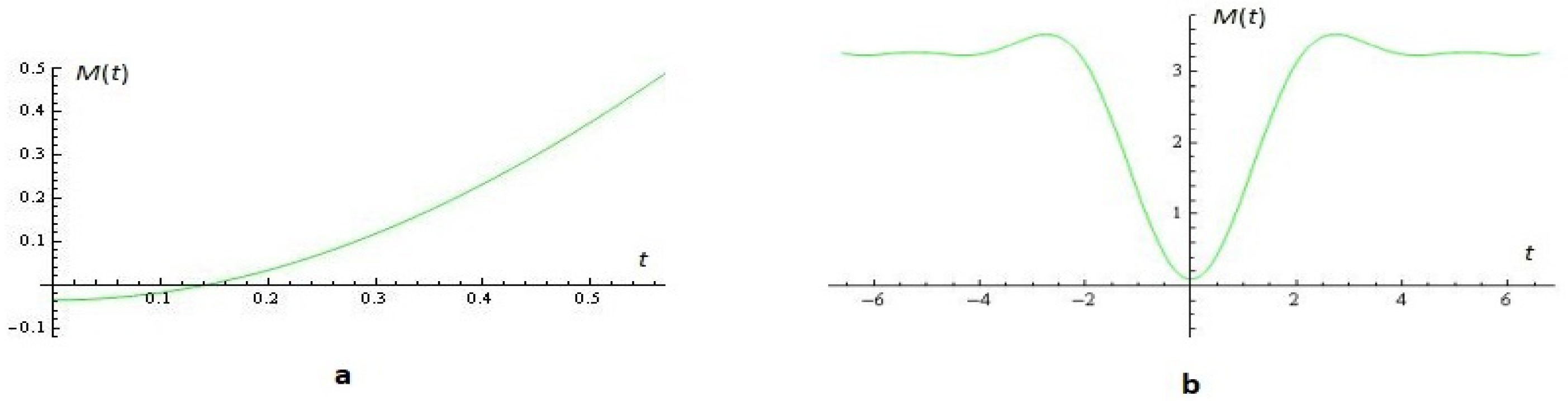
Proposition 1. 

If $m=n=3$ and $N=1$, then the Melnikov function $M\left(t_0\right)$ has a root which is calculated from the nonlinear equation

$$\frac{4}{3}\alpha -\frac{1}{6}{g}_1\pi {\omega }^2(6a+a_0(4+{\omega }^2))csch\left(\frac{\pi \omega }{2}\right)cos\left(t_0\omega \right)=0.$$

(6)

For example, for $\alpha =1.39627,a_0=1.2,a=1,\omega =2.2,$ and $g_1=0.7$, the root of the nonlinear Equation (6) is $t_0\approx 0.0003209$ with multiplicity two (see Figure 3).

Remark 1. 

If $M\left(t_0\right)=0$ and $\frac{dM\left(t_0\right)}{d{t}_0}\ne 0$ for some $t_0$ and some sets of parameters, then chaos occurs. This Melnikov criterion for the appearance of the intersection between the perturbed and unperturbed separatrixes leads to the following condition for chaotic behavior

$$g_1>\left|\frac{P}{Q}\right|,$$

where

$$\begin{array}{cc}\hfill P& =-\frac{1}{6}\pi {\omega }^2(6a+a_0(4+{\omega }^2))csch\left(\frac{\pi \omega }{2}\right)\hfill \\ \hfill Q& =\frac{4}{3}\alpha .\hfill \end{array}$$

It is important to note that a large region of parameter space will satisfy this inequality.

3.2. The Case n = m = 3 and N = 2

Similarly to Proposition 1, we can prove the following proposition when $n=m=3$ and $N=2$.

Proposition 2. 

If $m=n=3$ and $N=2$, then the Melnikov function $M\left(t_0\right)$ has a root which is a solution of the nonlinear equation

$$\begin{array}{ccc}M\left(t_0\right)\hfill & =& -\frac{1}{6}{e}^{-2i{t}_0\omega }csch\left(\pi \omega \right)\left(e^{i{t}_0\omega }(1+e^{2i{t}_0\omega })g_1\pi {\omega }^2(6a+a_0(4+{\omega }^2))cosh\left(\frac{\pi \omega }{2}\right)\right.\hfill \\ \hfill & & \left.+4((1+e^{4i{t}_0\omega })g_2\pi {\omega }^2(3a+2a_0(1+{\omega }^2))-2\alpha e^{2i{t}_0\omega }sinh\left(\pi \omega \right))\right)=0.\hfill \end{array}$$

(7)

3.3. The Case n = m = 3 and N = 3

The same approach leads to the following statement when $n=m=3$ and $N=3$.

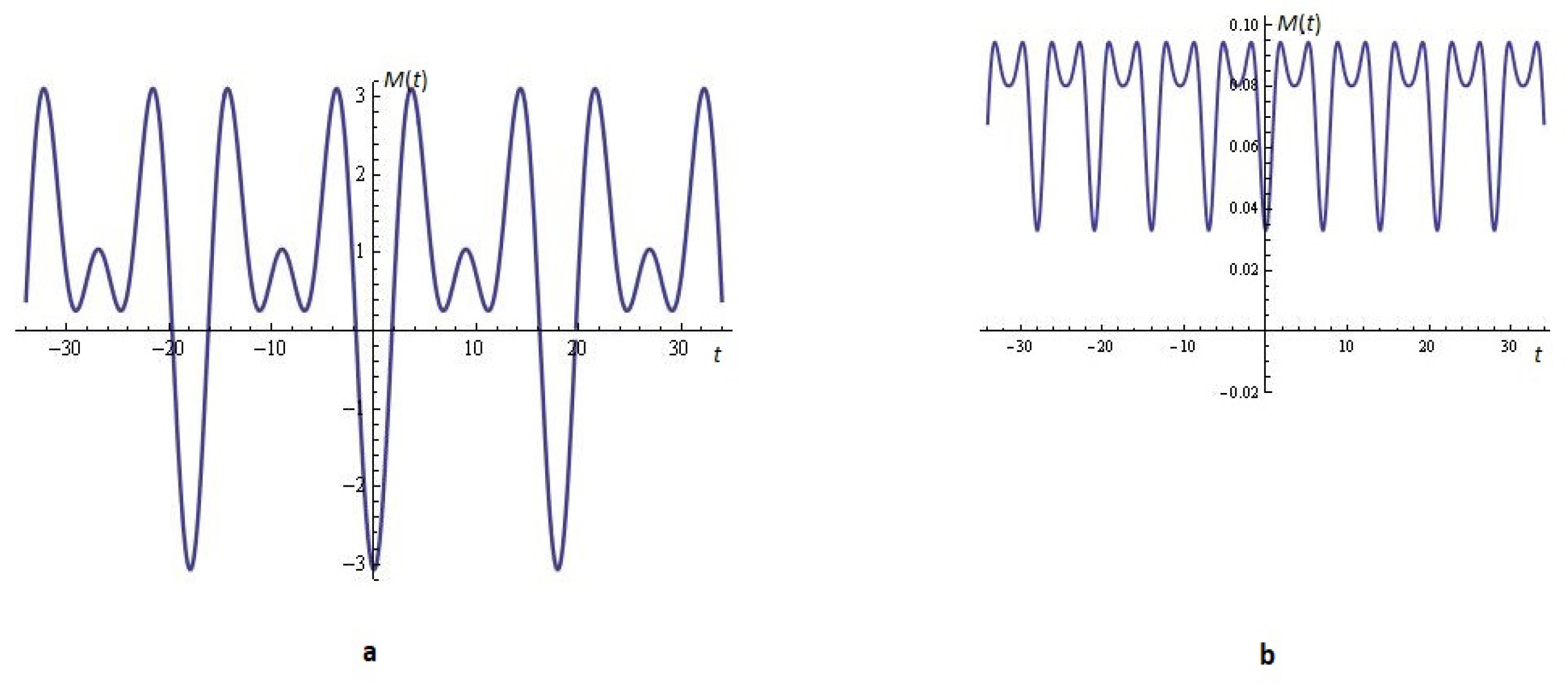
Proposition 3. 

If $m=n=3$ and $N=3$, then the root of Melnikov function (4) can be obtained via the nonlinear equation

$$\begin{array}{ccc}M\left(t_0\right)\hfill & =& -\frac{1}{24(1+2cosh(\pi \omega \left)\right)}{e}^{-3i{t}_0\omega }csch\left(\frac{\pi \omega }{4}\right)sech\left(\frac{\pi \omega }{4}\right)sech\left(\frac{\pi \omega }{2}\right)\times \hfill \\ \hfill & & \left((1+e^{2i{t}_0\omega })\pi {\omega }^2\left(6a\left(e^{2i{t}_0\omega }(2g_1-9g_3)+9g_3+9e^{4i{t}_0\omega }{g}_3\right)\right.\right.+\hfill \\ \hfill & & +a_0\left(9g_3(4+9{\omega }^2)+9e^{4i{t}_0\omega }{g}_3(4+9{\omega }^2)+\right.\hfill \\ \hfill & & \left.\left.+e^{2i{t}_0\omega }\left(2g_1(4+{\omega }^2)-9g_3(4+9{\omega }^2)\right)\right))\right)cosh\left(\frac{\pi \omega }{2}\right)+\hfill \\ \hfill & & +e^{i{t}_0\omega }\left(8(1+e^{4i{t}_0\omega })g_2\pi {\omega }^2(3a+2a_0(1+{\omega }^2))cosh\left(\pi \omega \right)+\right.\hfill \\ \hfill & & +e^{i{t}_0\omega }(1+e^{2i{t}_0\omega })g_1\pi {\omega }^2(6a+a_0(4+{\omega }^2))cosh\left(\frac{3\pi \omega }{2}\right)+\hfill \\ \hfill & & +4((1+e^{4i{t}_0\omega })g_2\pi {\omega }^2(3a+2a_0(1+{\omega }^2))-\hfill \\ \hfill & & \left.\left.\left.\left.-2\alpha e^{2i{t}_0\omega }sinh\left(\pi \omega \right)-2\alpha e^{2i{t}_0\omega }sinh\left(2\pi \omega \right)\right)\right)\right)\right)=0.\hfill \end{array}$$

(8)

For example, for $\alpha =1.7,a_0=0.8,a=1,\omega =0.75,g_1=0.7,g_2=0.3,$ and $g_3=0.1$, the root of the nonlinear Equation (8) is $t_0\approx 0.144$ (see Figure 4).

4. Open Problems

Problem 1. 

The reader can consider the corresponding approximation problem for arbitrarily chosen $n,m$ and N.

For $n>3$, the study of the critical levels of the Hamiltonian $H(x,y)$ is very complicated. In this regard, we recommend the study of Gavrilov and Iliev [31]. Note that even with the weakened choice $n=3$ and $m,N$ sufficiently large numbers, some difficulties (of a user nature) are encountered when calculating the Melnikov integrals using known Computer Algebraic Systems.

Problem 2. 

The Melnikov function $M\left(t_0\right)$ can be evaluated via the method of residuals.

Modern computer algebraic systems for scientific calculations provide this opportunity for the users. The upgrade of the Web application planned by us foresees the use of an algorithm (hidden to the user) to define the limit of the type $\left|Im\right(\omega \left)\right|\le Const$. For example, see Proposition 3, we calculate $M\left(t_0\right)$ but with a pre-set limit by us: $\left|Im\left(\omega \right)\right|\le \frac{2}{3}$.

5. Some Simulations

Here, we will focus on some interesting simulations.

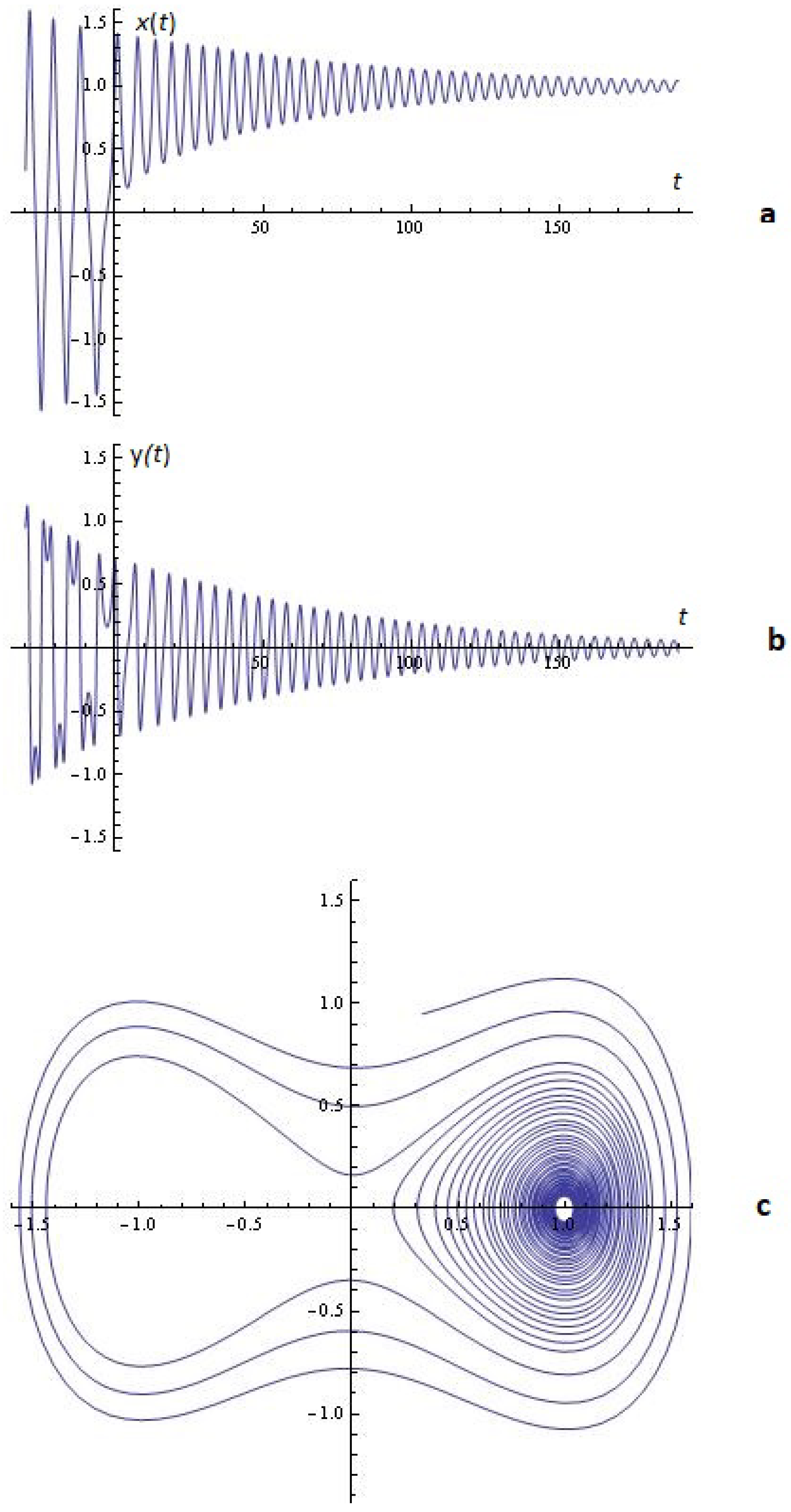
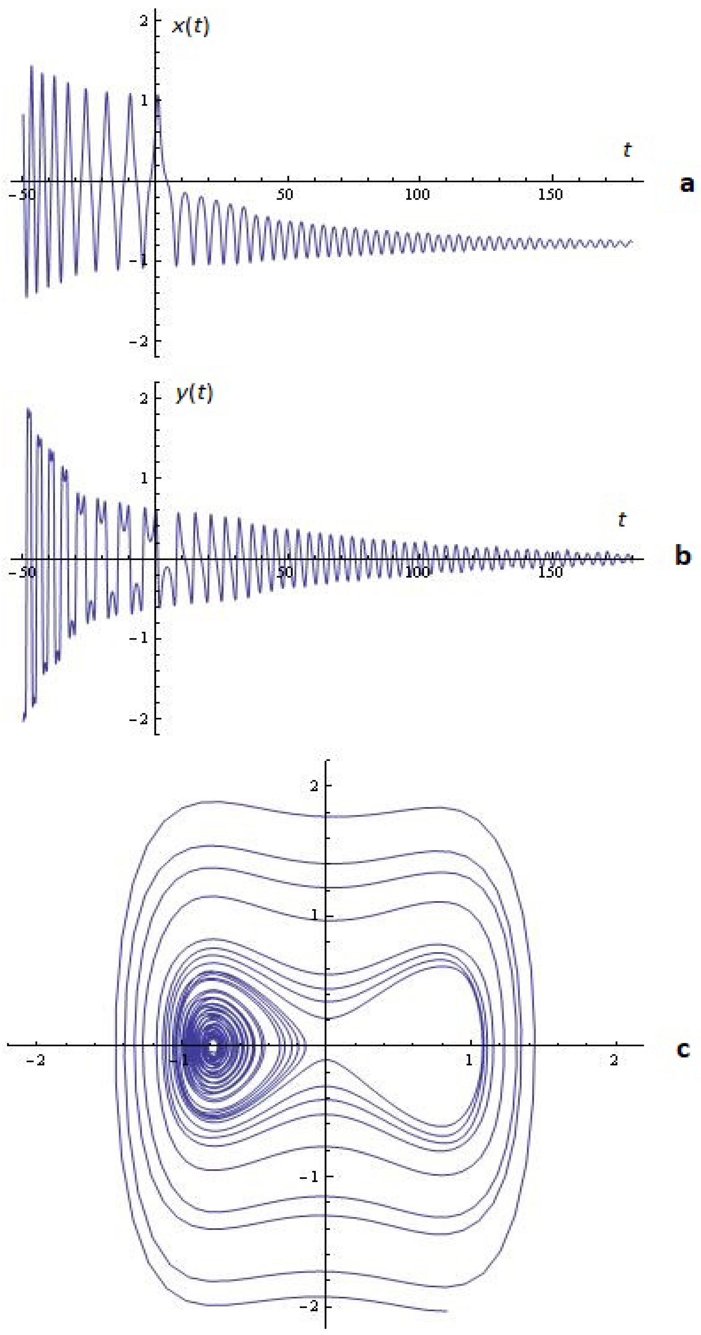
Example 1. For the given $n=m=3$, $N=3$, $a=1,\alpha =2.7,a_0=-1.2,b=b_0=1,$$ϵ=0.01,$$\omega =2.2,g_1=0.7,g_2=0.8,$ and $g_3=0.9$ the simulations on the system (2) for $x_0=0.9$; $y_0=0.7$ are depicted in Figure 5.

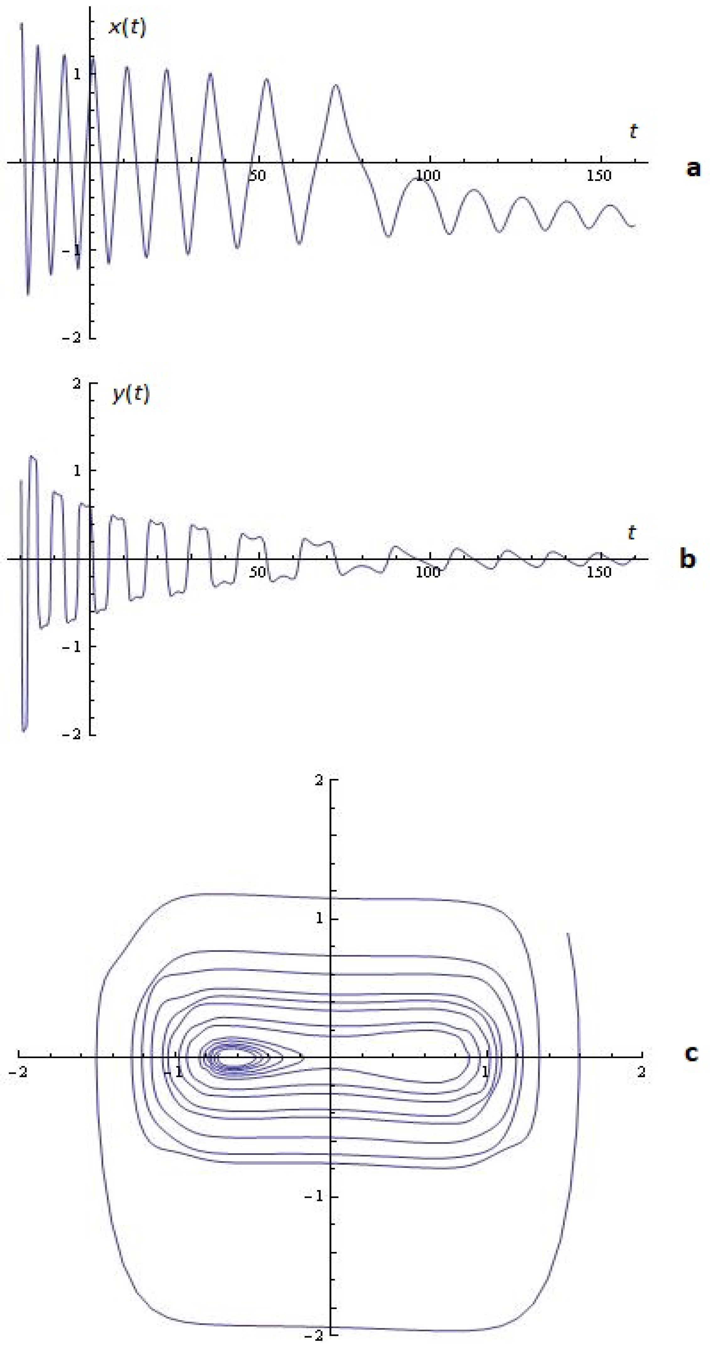
Example 2. For a given $n=m=5$, $N=4$, $a=1,\alpha =2.9,a_0=-3.35,a_1=-2.2,b=b_0=b_1=1,ϵ=0.01,\omega =2.1,g_1=0.9.g_2=1.1,g_3=1.6,$ and $g_4=2.5,$ the simulations on the system (2) for $x_0=0.7$; $y_0=0.6$ are depicted in Figure 6.

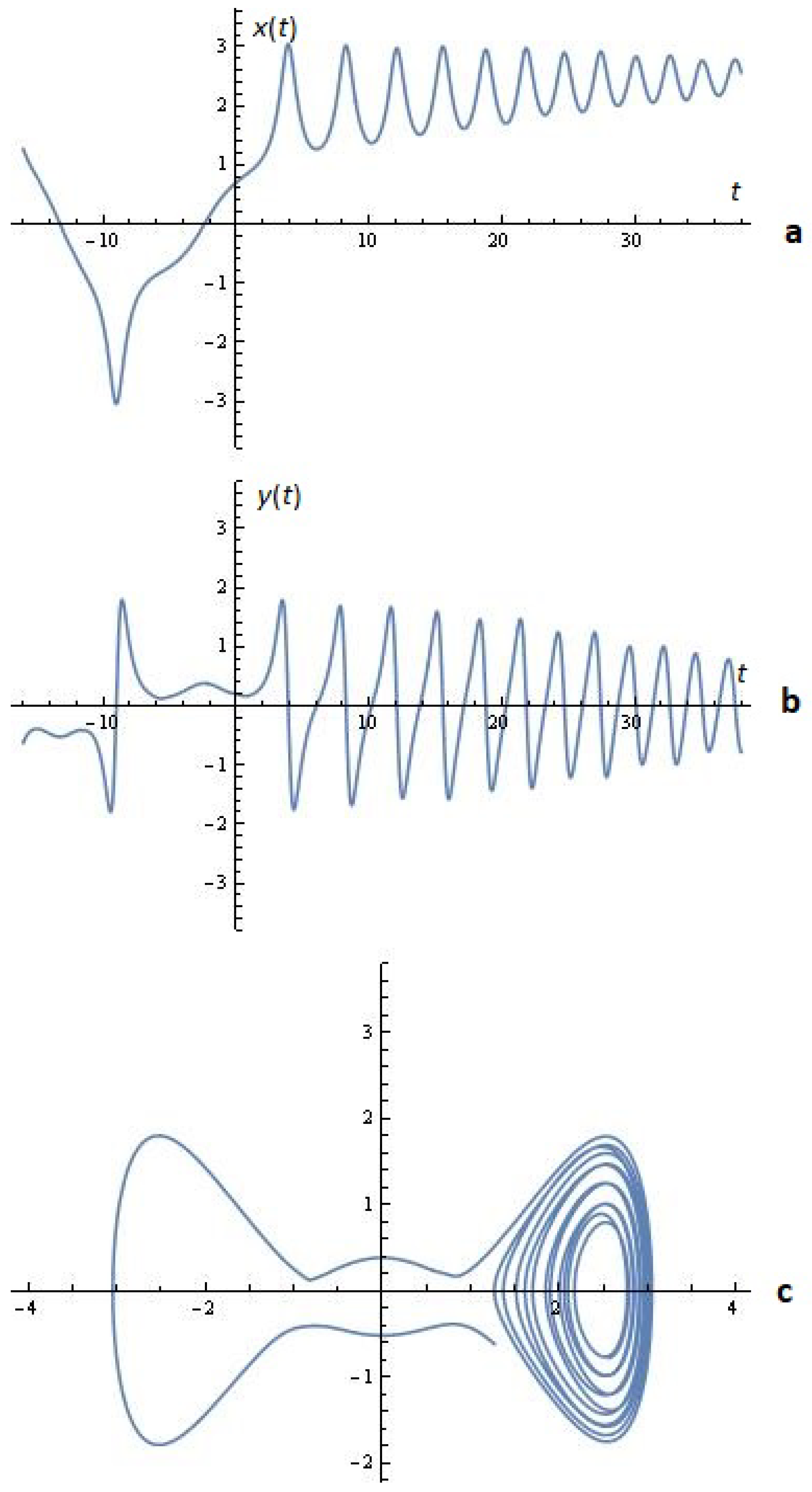
Example 3. For a given $n=m=7$, $N=4$, $a=1,\alpha =2.9,a_0=-3.35,a_1=-3.35,$ $a_2=-1.5,$ $b=0.1,$ $b_0=0.3,b_1=0.01,b_2=0.2,ϵ=0.01,\omega =2.1,g_1=0.9.g_2=1.1,$ $g_3=1.6,$ and $g_4=2.5$, the simulations on the system (2) for $x_0=0.7$; $y_0=0.6$ are depicted in Figure 7.

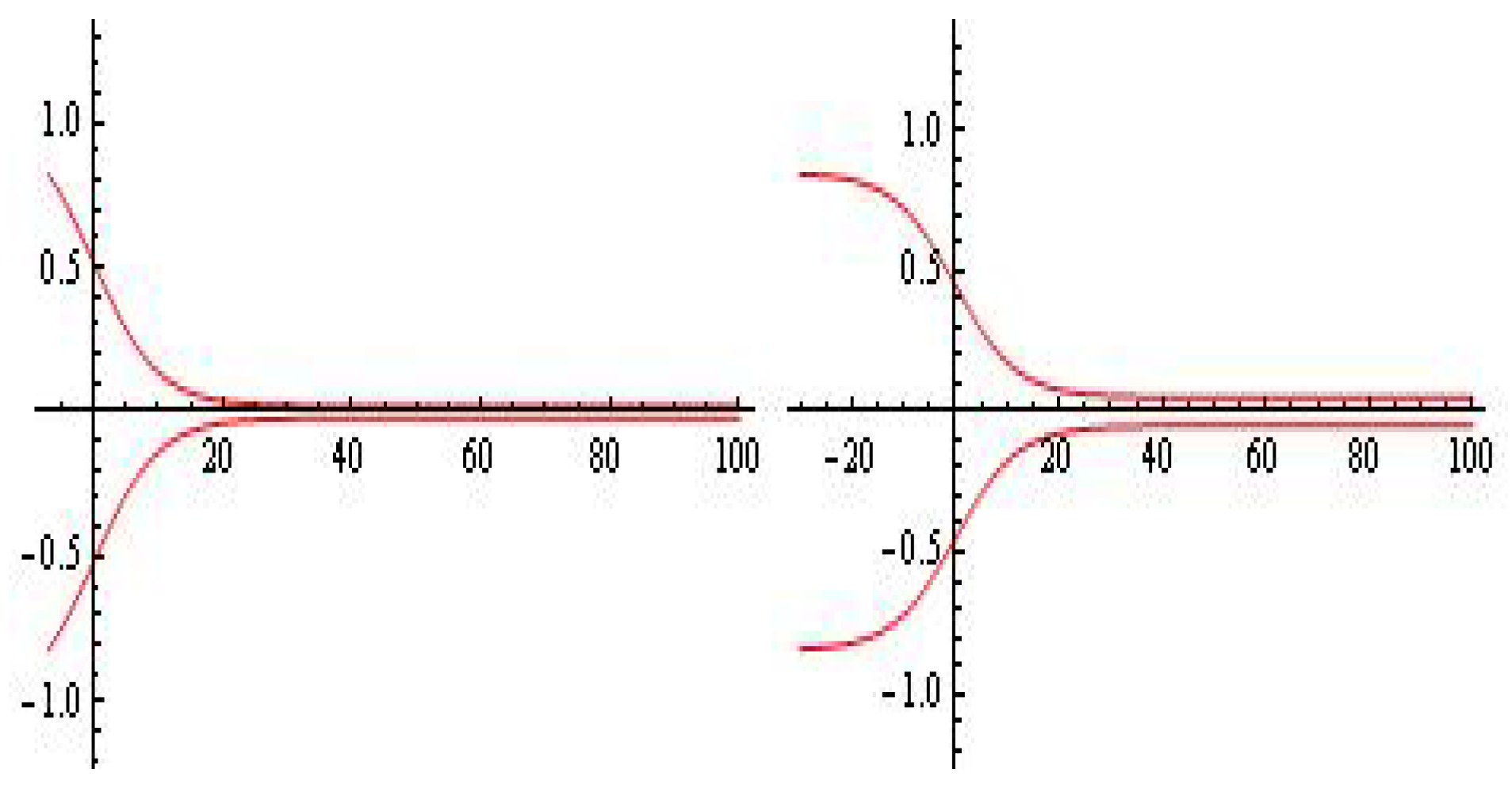
Problem 3. 

The task of researching the schematic implementation (design, fabrication, etc.) of the considered differential model can be considered open.

Note that one of the possibilities for conducting qualitative experimental studies for fabricated micro-electromechanical oscillator systems of type (2) and verifying their chaotic behavior is the use of some classical methods from the field of approximation theory, particularly from the direction approximations with constraints.

The characteristic restrictions for this class of oscillators, more precisely on the y-component of the differential model solution, are visualized in Figure 8.

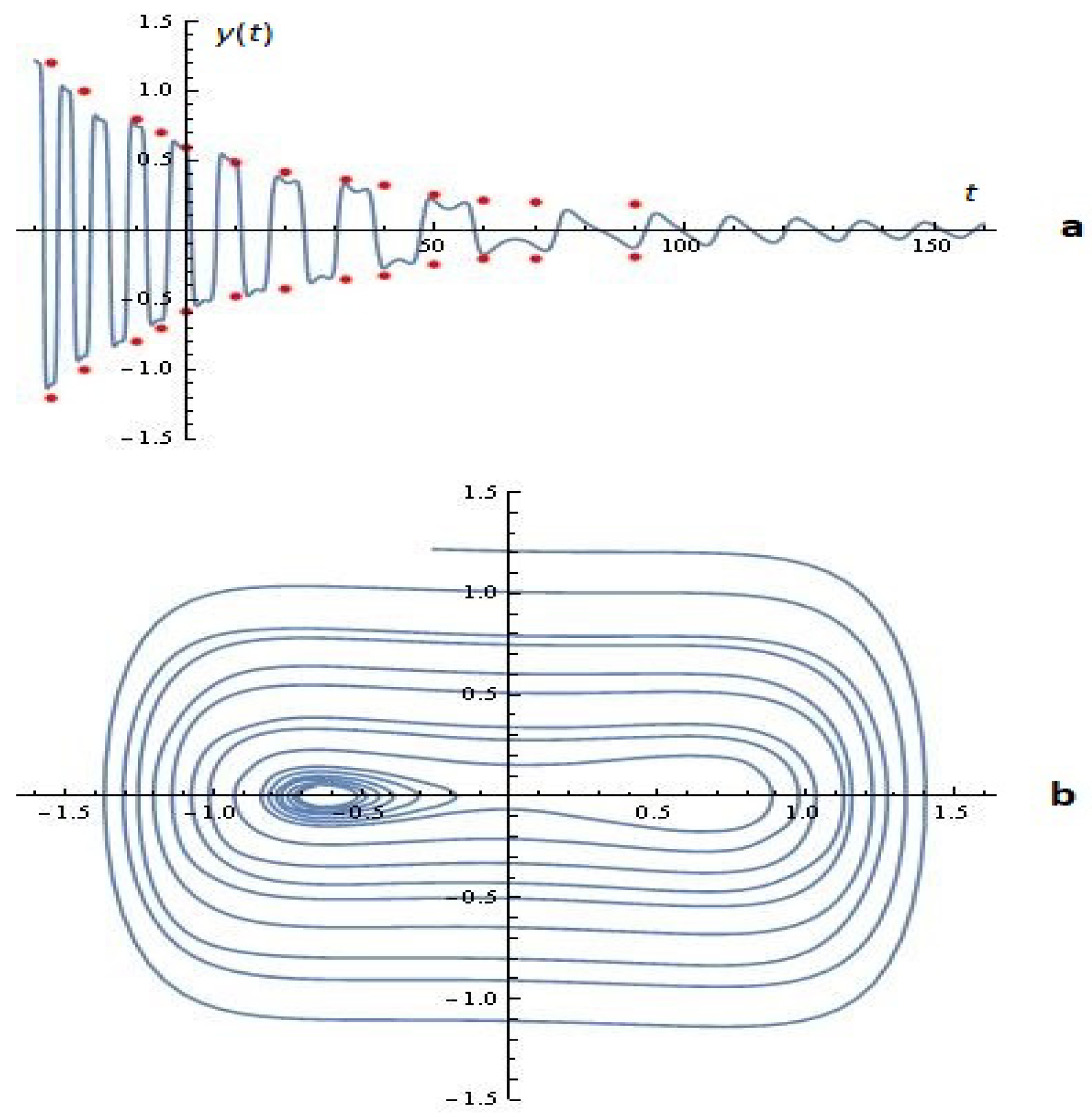
Let us present one more example. With the fixed values of the parameters from Example 3, but with the special choice of the parameters $g_i$ of the form: $g_i=0.9-0.2(i-1);$ $i=1,2,3,4$ (or a similar uniform network), a relatively good hit in the restriction fork is achieved (see Figure 9a).

5.1. Parameters Generated by a Probability Distribution

An alternative to control the mentioned chaotic behavior is to study this class of oscillators under probability distributed parameters $a_i$, $i=0,1,\dots ,\left[\frac{m}{2}\right]$, $b_i$, $i=0,1,\dots ,\left[\frac{n}{2}\right]$, $g_j$, $j=1,2,\dots ,N$. Of course, many distributions can be considered, but we focus mainly on two examples—binomial and truncated geometric. The first one is proposed since its asymptotic behavior is the normal distribution, which may be the most used in all practical fields. In addition, the truncated geometric distribution is suggested, because the original geometric distribution is the unique discrete one which exhibits the property memoryless—a necessary feature for many real-life fields. This way, the values of $a_i$, $b_i$, and $g_i$ can be calculated through the probability mass functions of the mentioned above distributions—we denote them by $p_{bin}$ and $p_{TG}$. If we assume that their support is $\left\{0,1,2,\dots ,M\right\}$, then they are

$$\begin{array}{cc}\hfill p_{bin}\left(k\right)& =\left(\genfrac{}{}{0pt}{}{M}{k}\right)p^k{\left(1-p\right)}^{M-k},k\in \left\{0,1,2,\dots ,M\right\},0<p<1\hfill \\ \hfill p_{TG}\left(k\right)& =\frac{p{\left(1-p\right)}^k}{1-{\left(1-p\right)}^{M+1}},k\in \left\{0,1,2,\dots ,M\right\},0<p<1.\hfill \end{array}$$

(9)

Thus, the necessary coefficients $a_i$, $b_i$, and $g_i$ can be set to be equal to the corresponding values $p_{bin}\left(k\right)$ or $p_{TG}\left(k\right)$.

6. An Example with a Relatively Large Number of Terms: n = 5, m = 5

We suppose now that $n=m=5$, and consider the model (2) for $b<0,b_1<0,b_0>0$. For $ϵ=0$, the resulting Hamiltonian of the system (2) is

$$H(x,y)=\frac{1}{2}{y}^2-\frac{1}{2}b{x}^2+\frac{1}{4}{b}_1{x}^4+\frac{1}{6}{b}_0{x}^6.$$

The potential energy

$$V\left(x\right)=-\frac{1}{2}b{x}^2+\frac{1}{4}{b}_1{x}^4+\frac{1}{6}{b}_0{x}^6$$

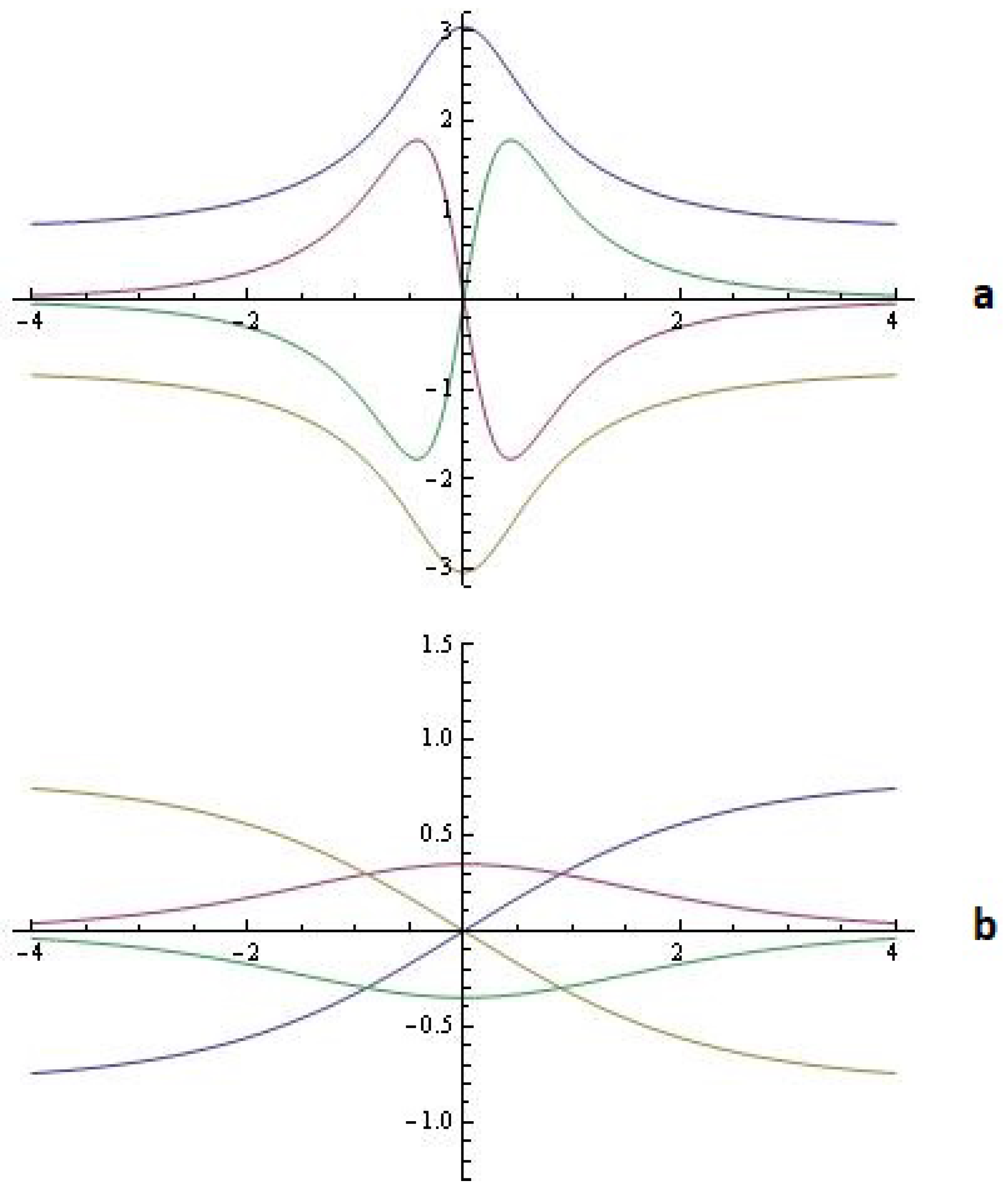
is shown in Figure 10. In [32], the authors study the resonant oscillation and the homoclinic bifurcation in a ${\varphi }^6$—Van der Pol oscillator. Following the ideas given in [32], we obtain the Hamiltonian system for $ϵ=0$ for our model (2) through a pair of heteroclinic orbits defined as (Figure 11b)

$$\begin{array}{cc}\hfill x_{het}& =\pm \frac{\sqrt{2}{x}_{1}sinh\left(\frac{\gamma }{2}t\right)}{\sqrt{-\xi +cosh\left(\gamma t\right)}}\hfill \\ \hfill y_{het}& =\pm \frac{\sqrt{2}\gamma x_1(1-\xi )cosh\left(\frac{\gamma }{2}t\right)}{2{(-\xi +cosh\left(\gamma t\right))}^{\frac{3}{2}}}\hfill \end{array}$$

and a pair of symmetric homoclinic trajectories connected each unstable point to itself given by (Figure 11a)

$$\begin{array}{cc}\hfill x_{hom}& =\pm \frac{\sqrt{2}{x}_{1}cosh\left(\frac{\gamma }{2}t\right)}{\sqrt{\xi +cosh\left(\gamma t\right)}};\hfill \\ \hfill y_{hom}& =\pm \frac{\sqrt{2}\gamma x_1(\xi -1)sinh\left(\frac{\gamma }{2}t\right)}{2{(\xi +cosh\left(\gamma t\right))}^{\frac{3}{2}}},\hfill \end{array}$$

where

$$\begin{array}{cc}\hfill \delta & =b_1^2+4b{b}_0\hfill \\ \hfill \rho & =\sqrt{\frac{b_1-\sqrt{\delta }}{b_1+\sqrt{\delta }}}\hfill \\ \hfill \xi & =\frac{5-3{\rho }^2}{2{\rho }^2-1}\hfill \\ \hfill x_1& =\sqrt{-\frac{1}{2b_0}(b_1+\sqrt{\delta })}\hfill \\ \hfill \gamma & =x_1^2\sqrt{2b_0({\rho }^2-1)}.\hfill \end{array}$$

These results are presented in Figure 11. We refer to [32,33,34,35] for more details. Next, we present a few more illustrative examples.

Example 4. For a given $n=m=5$, $N=4$, $a=1,\alpha =0.1,a_1=0.1,$ $a_0=0.05,$ $b=-0.4,$ $b_0=0.1,b_1=-0.4,ϵ=0.01,\omega =1.1,g_1=0.9,g_2=0.6,g_3=0.3,$ and $g_4=0.01$, the simulations on system (2) for $x_0=0.6$; $y_0=0.2$ are depicted in Figure 12.

Example 5. With the fixed values of the parameters from Example 5, but with the special choice of the parameters $g_i$ of the form: $g_1=1.7,g_2=1.5,g_3=1.3,$ $g_4=1,$ and $g_5=0.7$, the simulations on system (2) for $x_0=0.7$; $y_0=0.2$ are depicted in Figure 13.

We have to note that the calculation of homoclinic and heteroclinic Melnikov integrals as well as the corresponding criterion for the chaos occurrence in the dynamical system (for $n=m=5$, $N\ge 4$) are problematic tasks for users. For other problems of a computational nature, see [35].

7. Some Difficulties That the User Encounters When Using Computer Algebraic Systems for Scientific Calculation

Here, we will focus only on those difficulties that the user encounters when calculating homoclinic Melnikov integrals.

First of all, we will note that the user (who is not necessarily to be a professional mathematician) can hardly find out what option to choose for the mandatory field in the existing specialized module (for example, in CAS Mathematica) for calculating the above-mentioned integrals. Usually, this requirement is related to the imposed constraint (for the class of dynamical models) of type $\left|Im\right(\omega \left)\right|\le Const$ (see Section 4). The upgrade of the Web application planned by us foresees the use of an algorithm (hidden for the user) to define the limit of the above-mentioned constraint.

In a number of cases, a comment message appears (after a long pause) of the type: “No more memory available”, or ”SystemException[MemoryAllocationFailure, …]”, which is not particularly useful information for the nonprofessional user.

We note that when calculating the mentioned integrals for large values of the parameters in the considered differential model, the following comment message often appears: “A very large output was generated. Here is a simple of it:”. In this situation, the user’s hands are tied again.

We will give one more example (our unpublished result) related to studying the dynamics of an extended escape model of the form:

$$\left\{\begin{array}{ccc}{\displaystyle \frac{dx}{dt}}\hfill & =& y\hfill \\ {\displaystyle \frac{dy}{dt}}\hfill & =& -x+x^2-ϵ\left(A{\displaystyle \sum _{p=1}^n}y{\left|y\right|}^{p-1}+{\displaystyle \sum _{j=1}^N}{g}_{j}sin\left(j\omega t\right)\right)\hfill \end{array}\right.$$

(10)

where $0\le ϵ<1$, A is the damping level, $p\ge 1$ is the damping exponent, and N is the integer. In particular, we consider the following model

$$\left\{\begin{array}{ccc}{\displaystyle \frac{dx}{dt}}\hfill & =& y\hfill \\ {\displaystyle \frac{dy}{dt}}\hfill & =& -x+x^2-ϵ\left({Ay\left|y\right|}^{p-1}+{\displaystyle \sum _{j=1}^N}{g}_{j}sin\left(j\omega t\right)\right),\hfill \end{array}\right.$$

(11)

The following statement is valid.

Proposition 4. 

If $p=2$ and $N=3$, then the roots of Melnikov function $M\left(t_0\right)$ are given as solutions of the equation

$$\begin{array}{ccc}M\left(t_0\right)\hfill & =\hfill & \frac{1}{60}{e}^{-3i{t}_0\omega }\left(32\sqrt{2}A{e}^{3i{t}_0\omega }+15\sqrt{2}{e}^{2i{t}_0\omega }{g}_1\omega PolyGamma[0,\frac{1}{4}-\frac{i\omega }{4}]\right.\hfill \\ \hfill & \hfill & +15\sqrt{2}{e}^{4i{t}_0\omega }{g}_1\omega PolyGamma[0,\frac{1}{4}-\frac{i\omega }{4}]-15\sqrt{2}{e}^{2i{t}_0\omega }{g}_1\omega PolyGamma[0,\frac{3}{4}-\frac{i\omega }{4}]\hfill \\ \hfill & \hfill & -15\sqrt{2}{e}^{4i{t}_0\omega }{g}_1\omega PolyGamma[0,\frac{3}{4}-\frac{i\omega }{4}]+15\sqrt{2}{e}^{2i{t}_0\omega }{g}_1\omega PolyGamma[0,\frac{1}{4}+\frac{i\omega }{4}]\hfill \\ \hfill & \hfill & +15\sqrt{2}{e}^{4i{t}_0\omega }{g}_1\omega PolyGamma[0,\frac{1}{4}+\frac{i\omega }{4}]-15\sqrt{2}{e}^{2i{t}_0\omega }{g}_1\omega PolyGamma[0,\frac{3}{4}+\frac{i\omega }{4}]\hfill \\ \hfill & \hfill & -15\sqrt{2}{e}^{4i{t}_0\omega }{g}_1\omega PolyGamma[0,\frac{3}{4}+\frac{i\omega }{4}]+30\sqrt{2}{e}^{i{t}_0\omega }{g}_2\omega PolyGamma[0,\frac{1}{4}-\frac{i\omega }{2}]\hfill \\ \hfill & \hfill & +30\sqrt{2}{e}^{5i{t}_0\omega }{g}_2\omega PolyGamma[0,\frac{1}{4}-\frac{i\omega }{2}]-30\sqrt{2}{e}^{i{t}_0\omega }{g}_2\omega PolyGamma[0,\frac{3}{4}-\frac{i\omega }{2}]\hfill \\ \hfill & \hfill & -30\sqrt{2}{e}^{5i{t}_0\omega }{g}_2\omega PolyGamma[0,\frac{3}{4}-\frac{i\omega }{2}]+30\sqrt{2}{e}^{i{t}_0\omega }{g}_2\omega PolyGamma[0,\frac{1}{4}+\frac{i\omega }{2}]\hfill \\ \hfill & \hfill & +30\sqrt{2}{e}^{5i{t}_0\omega }{g}_2\omega PolyGamma[0,\frac{1}{4}+\frac{i\omega }{2}]-30\sqrt{2}{e}^{i{t}_0\omega }{g}_2\omega PolyGamma[0,\frac{3}{4}+\frac{i\omega }{2}]\hfill \\ \hfill & \hfill & -30\sqrt{2}{e}^{5i{t}_0\omega }{g}_2\omega PolyGamma[0,\frac{3}{4}+\frac{i\omega }{2}]+45\sqrt{2}{g}_3\omega PolyGamma[0,\frac{1}{4}-\frac{3i\omega }{4}]\hfill \\ \hfill & \hfill & +45\sqrt{2}{e}^{6i{t}_0\omega }{g}_3\omega PolyGamma[0,\frac{1}{4}-\frac{3i\omega }{4}]-45\sqrt{2}{g}_3\omega PolyGamma[0,\frac{3}{4}-\frac{3i\omega }{4}]\hfill \\ \hfill & \hfill & -45\sqrt{2}{e}^{6i{t}_0\omega }{g}_3\omega PolyGamma[0,\frac{3}{4}-\frac{3i\omega }{4}]+45\sqrt{2}{g}_3\omega PolyGamma[0,\frac{1}{4}+\frac{3i\omega }{4}]\hfill \\ \hfill & \hfill & +45\sqrt{2}{e}^{6i{t}_0\omega }{g}_3\omega PolyGamma[0,\frac{1}{4}+\frac{3i\omega }{4}]-45\sqrt{2}{g}_3\omega PolyGamma[0,\frac{3}{4}+\frac{3i\omega }{4}]\hfill \\ \hfill & \hfill & \left.-45\sqrt{2}{e}^{6i{t}_0\omega }{g}_3\omega PolyGamma[0,\frac{3}{4}+\frac{3i\omega }{4}]\right)=0.\hfill \end{array}$$

(12)

where $PolyGamma[n,z]$ gives the $n^{th}$ derivative of the digamma function ${\psi }^{\left(n\right)}\left(z\right)$, i.e., ${\psi }^{\left(0\right)}\left(z\right)=\frac{{\Gamma }^{\prime }\left(z\right)}{\Gamma \left(z\right)}$ and $\Gamma \left(z\right)={\displaystyle {\int }_0^{\infty }}{t}^{z-1}{e}^{-t}dt$ (see, for example, [36]).

For example, the equation $M\left(t_0\right)=0$ (for $p=2;N=3;A=1.01;\omega =0.35;$ $g_1=0.5;$ $g_2=0.95;g_3=0.8$) is depicted in Figure 14.

Of course, the user can make some simplifications in Equation (12) himself. But naturally, the question arises as to why, for example, the existing HarmonicNumber[n] operator (in the specified programming environment) was not used (automatically) to obtain a compact record. The examples we can cite are many and varied. This necessitates the professional upgrading of the existing specialized modules.

8. Concluding Remarks

We have investigated in this paper a generalized differential model for micro-electromechanical oscillators in the light of Melnikov’s approach. The derived results can be used to estimate the associated total energy potential of the considered differential system. Nonstandard numerical methods connected to deriving the roots of the nonlinear equation $M\left(t_0\right)=0$ can be found in [37,38,39]. In some cases (when generating chaos in dynamical systems via $x\left|x\right|$), $M\left(t\right)$ is of polynomial type. Numerical methods for solving polynomial equations can be found in [40,41,42,43,44]. Some dynamic modules implemented in CAS Wolfram Mathematica for investigating the dynamics of some new hypothetical oscillators have been demonstrated. A cloud version that requires only a browser and internet connection is offered for some of them. They will be an integral part of the above-mentioned Web-based application for scientific computing. Let us note that the theoretical apparatus for studying the circuit implementation (design, fabricating, etc.) of the considered differential model is extremely complex and requires a serious investigation before being adapted for its possible inclusion in our planned Web platform. Other interesting problems are posed in the article [45]. Questions related to the computer and hardware modeling of periodically forced oscillators discussed in Section 6, especially for large values of N, can be considered open.

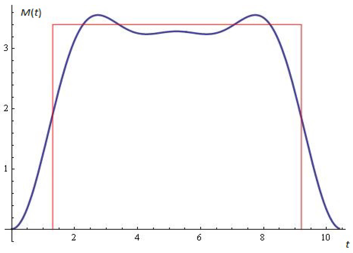
In a number of cases, Melnikov’s function $M\left(t\right)$ can be used to approximate rectangular-type signals (see Figure 15) as well as to synthesize digital filters. Melnikov’s function $M\left(t\right)$ as a typical emitting diagram is depicted in Figure 16. For some details, see [46]. Such reviews will also be the subject of our planned Web application.

Our planned platform implements the following: the Melnikov functions of higher kind for analysis of homo/heteroclinic bifurcation in mechanical systems; bifurcation diagrams; and chaos in a nonautonomous system. Some of these algorithms are based on known classical and more recent research [6,7,8,9,10,11,12,13,20]. These modules are improving on similar ones realized in computer algebraic systems designed for scientific calculations.

We fully understand that the construction of such an ambitious Web-based platform for scientific computing can only be realized with the active participation of specialists from various branches of scientific knowledge.

Future investigations. We have plans to explore modified escape oscillators of the form:

$$\left\{\begin{array}{ccc}{\displaystyle \frac{dx}{dt}}\hfill & =& y\hfill \\ {\displaystyle \frac{dy}{dt}}\hfill & =& -Poly\left(x\right)-ϵ\left(A{\displaystyle \sum _{p=1}^n}y{\left|y\right|}^{p-1}+{\displaystyle \sum _{j=1}^N}{g}_{j}sin\left(j\omega t\right)\right),\hfill \end{array}\right.$$

where $0\le ϵ<1$, A is the damping level, $p\ge 1$ is the damping exponent, N is the integer and $Poly\left(x\right)=\left\{P\right(x),H(x),T(x),U(x\left)\right\}$ where $P\left(x\right),H\left(x\right),T\left(x\right),U\left(x\right)$ are Legendre, Hermite, Chebyshev (first kind) and Chebyshev (second kind) polynomials, respectively.

We envisage the study of such interesting dynamic models to be implemented in the Web application cited above.

References

- Zounes, R.; Rand, R. Subharmonic resonance in the nonlinear Mathieu equation. Int. J. Non-Linear Mech. 2002, 37, 43–73. [Google Scholar] [CrossRef]
- DeMartini, B.; Butterfield, H.; Moehlis, J.; Turner, K. Chaos for a microelectromechanical oscillator governed by the nonlinear Mathieu equation. J. Microelectromech. Syst. 2007, 16, 1314–1323. [Google Scholar] [CrossRef]
- DeMartini, B.; Moehlis, J.; Turner, K.; Rhoads, J.; Shaw, S.; Zhang, W. Modelling of parametrically excited microelectromechanical oscillator dynamics with application to filtering. In Proceedings of the IEEE Sensors Conference, Irvine, CA, USA, 30 October–3 November 2005; pp. 345–348. [Google Scholar]
- Luo, A.; Wang, F. Nonlinear dynamics of a micro-electro-mechanical system with time-varying capacitors. J. Vib. Acoust. 2004, 126, 77–83. [Google Scholar] [CrossRef]
- Wiggins, S. Introduction to Applied Nonlinear Dynamical Systems and Chaos, 2nd ed.; Springer: New York, NY, USA, 2003. [Google Scholar]
- Lenci, S.; Lupini, R. Homoclinic and heteroclinic solutions for a class of two-dimensional Hamiltonian systems. Z. Angew. Math. Phys. 1996, 47, 97–111. [Google Scholar] [CrossRef]
- Lenci, S.; Rega, G. Controlling nonlinear dynamics in a two-well impact system. I. Attractors and bifurcation scenario under symmetric excitations. Int. J. Bifurc. Chaos 1998, 8, 2387–2407. [Google Scholar] [CrossRef]
- Lenci, S.; Rega, G. Controlling nonlinear dynamics in a two-well impact system. II. Attractors and bifurcation scenario under unsymmetric optimal excitation. Int. J. Bifurc. Chaos 1998, 8, 2409–2424. [Google Scholar] [CrossRef]
- Lenci, S.; Rega, G. Higher-order Melnikov analysis of homo/heteroclinic bifurcations in mechanical oscillators. In Proceedings of the 16th AIMETA Congress of Theoretical and Applied Mechanics (Ferrara), Ferrara, Italy, 9–12 September 2003. CD-Rom. [Google Scholar]
- Lenci, S.; Rega, G. Optimal control of homoclinic bifurcation: Theoretical treatment and practical reduction of safe basin erosion in the Helmholtz oscillator. J. Vib. Control 2003, 9, 281–315. [Google Scholar] [CrossRef]
- Lenci, S.; Rega, G. Bifurcations and chaos in single-d.o.f. mechanical systems: Exploiting nonlinear dynamics properties for their control. In Recent Research Developments in Structural Dynamics; Luongo, A., Ed.; Research Signpost: Kerala, India, 2003; pp. 331–369. [Google Scholar]
- Soto-Trevino, C.; Kaper, T. Higher-order Melnikov theory for adiabatic systems. J. Math. Phys. 1996, 37, 6220–6249. [Google Scholar] [CrossRef]
- Thompson, M.; Stewart, H. Nonlinear Dynamics and Chaos, 2nd ed.; John Wiley & Sons: Chichester, UK, 2002. [Google Scholar]
- Kyurkchiev, N.; Zaevski, T. On a hypothetical oscillator: Investigations in the light of Melnikov’s approach, some simulations. Int. J. Differ. Equations Appl. 2023, 22, 67–79. [Google Scholar]
- Melnikov, V.K. On the stability of a center for time–periodic perturbation. Trans. Mosc. Math. Soc. 1963, 12, 1–57. [Google Scholar]
- Kyurkchiev, V.; Iliev, A.; Rahnev, A.; Kyurkchiev, N. On a class of orthogonal polynomials as corrections in Lienard differential system. Applications. Algorithms 2023, 16, 297. [Google Scholar] [CrossRef]
- Kyurkchiev, N.; Iliev, A. On the hypothetical oscillator model with second kind Chebyshev’s polynomial–correction: Number and type of limit cycles, simulations and possible applications. Algorithms 2022, 15, 462. [Google Scholar] [CrossRef]
- Vasileva, M.; Kyurkchiev, V.; Iliev, A.; Rahnev, A.; Kyurkchiev, N. Applications of Some Orthogonal Polynomials and Associated Polynomials of Higher Kind; Plovdiv University Press: Plovdiv, Bulgaria, 2023; ISBN 978-619-7663-72-3. [Google Scholar]
- Blows, T.; Perko, L. Bifurcation of Limit Cycles from Centers and Separatrix Cycles of Planar Analytic Systems. SIAM Rev. 1994, 36, 341–376. [Google Scholar] [CrossRef]
- Gavrilov, L.; Iliev, I. The limit cycles in a generalized Rayleigh–Lienard oscillator. Discret. Contin. Dyn. Syst. 2023, 43, 2381–2400. [Google Scholar] [CrossRef]
- Li, X.; Shen, Y.; Sun, J.; Yang, S. New periodic attractors is slow-fast Duffing system with periodic parametric excitation. Sci. Rep. 2019, 9, 11185. [Google Scholar] [CrossRef]
- Holmes, P.J. Chaos in Duffing’s equation: Strange Attractors? In Encyclopedia of Vibration; Braun, S.G., Ewins, D.J., Rao, S.S., Eds.; Academic Press: London, UK; San Diego, CA, USA, 2001; pp. 227–236. [Google Scholar]
- Sanchez, N.; Nayfeh, A. Prediction of bifurcations in a parametrically excited Duffing oscillator. Int. J. Nonlinear Mech. 1990, 25, 163–176. [Google Scholar] [CrossRef]
- Michon, G.; Manin, L.; Parker, R.; Dufour, R. Duffing oscillator with parametric excitation: Analytical and experimental investigation on a Belt–Pulley systems. ASME 2008, 3, 031001. [Google Scholar] [CrossRef]
- Yue, X.; Lv, G.; Zhang, Y. Rare and hidden attractors in a periodically forced Duffing system with absolute nonlinearity. Chaos Solitons Fractals 2021, 150, 111108. [Google Scholar] [CrossRef]
- Tang, K.; Man, K.; Zhong, G.; Chen, G. Generating chaos via x|x|. IEEE Trans. Circuits Syst. I Fundam. Theory Appl. 2001, 48, 636–641. [Google Scholar] [CrossRef]
- Guckenheimer, J.; Holmes, P. Nonlinear Oscillations, Dynamical Systems, and Bifurcations of Vector Fields; Sprinder: New York, NY, USA, 1983. [Google Scholar]
- Perko, L. Differential Equations and Dynamical Systems; Springer: New York, NY, USA, 1991. [Google Scholar]
- Holmes, P.; Marsden, J. Horseshoes in perturbation of Hamiltonian systems with two degrees of freedom. Comm. Math. Phys. 1982, 82, 523–544. [Google Scholar] [CrossRef]
- Holmes, P.; Marsden, J. A partial differential equation with infinitely many periodic orbits: Chaotic oscillations. Arch. Ration. Mech. Anal. 1981, 76, 135–165. [Google Scholar] [CrossRef]
- Gavrilov, L.; Iliev, I. Complete hyperelliptic integrals of the first kind and their non–oscillation. Trans. Am. Math. Soc. 2003, 356, 1185–1207. [Google Scholar] [CrossRef]
- Siewe, M.; Kakmeni, F.; Tchawoua, C. Resonant oscillation and homoclinic bifurcation in ϕ6—Van der Pol oscillator. Chaos Solut. Fractals 2004, 21, 841–853. [Google Scholar] [CrossRef]
- Adelakun, A.; Njah, A.; Olusola, O.; Wara, S. Computer and hardware modeling of periodically forced ϕ6—Van der Pol oscillator. Act. Passiv. Electron. Components 2016, 7, 3426713. [Google Scholar]
- Yu, J.; Li, J. Investigation on dynamics of the extended Duffing–Van der Pol system. Zetschrift Fur Naturforschung 2014, 64, 341–346. [Google Scholar] [CrossRef]
- Siewe, M.; Tchawoua, C.; Rajasekar, S. Homoclinic bifurcation and chaos in ϕ6 Rayleigh oscillator with three wells driven by an amplitude modulated force. Int. J. Bifurc. Chaos 2011, 21, 1583–1593. [Google Scholar] [CrossRef]
- Abramowicz, A.; Stegun, I. Handbook of Mathematical Functions; Dover: New York, NY, USA, 1970. [Google Scholar]
- Thangkhenpau, G.; Panday, S.; Bolunduet, L.C.; Jantschi, L. Efficient Families of Multi-Point Iterative Methods and Their Self-Acceleration with Memory for Solving Nonlinear Equations. Symmetry 2023, 15, 1546. [Google Scholar] [CrossRef]
- Akram, S.; Khalid, M.; Junjua, M.-U.-D.; Altaf, S.; Kumar, S. Extension of King’s Iterative Scheme by Means of Memory for Nonlinear Equations. Symmetry 2023, 15, 1116. [Google Scholar] [CrossRef]
- Cordero, A.; Janjua, M.; Torregrosa, J.R.; Yasmin, N.; Zafar, F. Efficient four parametric with and without-memory iterative methods possessing high efficiency indices. Math. Probl. Eng. 2018, 1–12. [Google Scholar] [CrossRef]
- Proinov, P.; Vasileva, M. Local and Semilocal Convergence of Nourein’s Iterative Method for Finding All Zeros of a Polynomial Simultaneously. Symmetry 2020, 12, 1801. [Google Scholar] [CrossRef]
- Proinov, P.; Ivanov, S. On the convergence of Halley’s method for simultaneous computation of polynomial zeros. J. Numer. Math. 2015, 23, 379–394. [Google Scholar] [CrossRef]
- Proinov, P.; Vasileva, M. On the convergence of high-order Gargantini-Farmer-Loizou type iterative methods for simultaneous approximation of polynomial zeros. Appl. Math. Comput. 2019, 361, 202–214. [Google Scholar] [CrossRef]
- Ivanov, S. Families of high-order simultaneous methods with several corrections. Numer. Algor. 2024. [Google Scholar] [CrossRef]
- Kyncheva, V.; Yotov, V.; Ivanov, S. Convergence of Newton, Halley and Chebyshev iterative methods as methods for simultaneous determination of multiple zeros. Appl. Numer. Math. 2017, 112, 146–154. [Google Scholar] [CrossRef]
- Stojanovic, V.; Petkovic, M.; Deng, J. Instability of vehicle systems moving along an infinite beam on a viscoelastic foundation. Eur. J. Mech.-A/Solids 2018, 69, 238–254. [Google Scholar] [CrossRef]
- Kyurkchiev, N.; Andreev, A. Approximation and Antenna and Filter Synthesis: Some Moduli in Programming Environment MATHEMATICA; LAP Lambert Academic Publishing: Saarbrucken, Germany, 2014; ISBN 978-3-859-53322-8. [Google Scholar]
Figure 1.
Double homoclinic orbit [
27].
Figure 2.
Potential energy .
Figure 3.
The nonlinear Equation (
6): (
a) for
,
has root
with multiplicity two; (
b) for
has no roots.
Figure 4.
8): (
; (
Figure 5.
(a) x-time series; (b) y-time series; (c) phase space; (Example 1).
Figure 6.
(a) x-time series; (b) y-time series; (c) phase space; (Example 2).
Figure 7.
(a) x-time series; (b) y-time series; (c) phase space; (Example 3).
Figure 8.
Possible restrictions.
Figure 9.
(a) y-time series (with restriction); (b) phase space; (Example 3).
Figure 10.
Potential energy for .
Figure 11.
For (a) homoclinic orbits; (b) heteroclinic orbits.
Figure 12.
(a) x-time series; (b) y-time series; (c) phase space; (Example 4).
Figure 13.
(a) x-time series; (b) y-time series; (c) phase space; (Example 5).
Figure 14.
The equation (Proposition 5.) for fixed parameters: (a) , , , , , , ; (b) , , , , , has no roots.
Figure 15.
Melnikov function (thick) for , , , , , , in interval [0,10] (see Proposition 3).
Figure 16.
Melnikov function for , , , , in interval (see Proposition 4).