Bertrand Offsets of Slant Ruled Surfaces in Euclidean 3-Space

Abstract

In this paper, we investigate and specify the Bertrand offsets of slant ruled and developable surfaces in Euclidean 3-space ${\mathcal{E}}^3$. This is accomplished by utilizing the symmetry of slant curves. As a consequence of this, we present the parameterization of the Bertrand offsets for any slant ruled and developable surfaces. In addition to this, we investigate the monarchies of these ruled surfaces and assign them their own unique classification. Also, we illustrate some examples of slant ruled surfaces.

1. Introduction

In the spatial kinematic, the locomotion of an oriented line embedded linked with a mobile solid body is mostly a ruled surface ($\mathcal{RS}$). As it is a significant theme of research in vintage differential geometry, it has been appraised by numerous scholars; see [1,2,3,4,5,6,7]. From the geometric point of view, the distinctive characteristics of ruled surfaces and their offset surfaces have been inspected in both Euclidean and non-Euclidean spaces. In the context of line geometry, Ravani and Ku released the theory of Bertrand ($\mathcal{B}$) curves for $\mathcal{RS}$ [8]. They showed that a $\mathcal{RS}$ can have an infinite number of Bertrand offsets ($\mathcal{BO}$), much as a plane curve can have an infinite number of $\mathcal{B}$ matches. Küçük and Gürsoy have specified some descriptions of $\mathcal{BO}$ of trajectory $\mathcal{RS}$ in view of the connections through the projection areas for the spherical curves of $\mathcal{BO}$ and their integral invariants [9]. In [10], Kasap and Kuruoglu obtained the interrelations through integral invariants of the couple of the $\mathcal{RS}$ in Euclidean 3-space ${\mathcal{E}}^3$. In [11], Kasap and Kuruoglu actuated the research of $\mathcal{BO}$ of $\mathcal{RS}$ in Minkowski 3-space. The involute–evolute offsets of $\mathcal{RS}$ were located by Kasap et al. in [12]. Orbay et al. [13] instigated the search of Mannheim offsets of the $\mathcal{RS}$. Onder and Ugurlu obtained the relationships through invariants of Mannheim offsets of timelike $\mathcal{RS}$, and they presented the issues for these surface offsets to be developable [14]. In view of the involute–evolute offsets of ruled surfaces, in [7], Senturk and Yuce designed integral invariants of these offsets via the geodesic Frenet frame [15]. More recently, Yoon explored evolute offsets of the $\mathcal{RS}$ in Minkowski 3-space ${\mathcal{E}}_1^3$ with stationary Gaussian curvature and mean curvature [16]. Also, Ref. [17] introduced some characterizations for a non-null $\mathcal{RS}$ to be a slant $\mathcal{RS}$ in ${\mathcal{E}}_1^3$, and described the relationships between a non-null slant $\mathcal{RS}$ and its striction line. M. Onder and O. Kaya in [18] obtained new characterizations for slant $\mathcal{RS}$ in the Euclidean 3-space. There exist a considerable number of written works on the topic of comprehensive diverse treatises; for instance, [19,20,21,22,23,24]. Nevertheless, to our knowledge, there is no work related to creating $\mathcal{BO}$ of slant $\mathcal{RS}$ via the geometrical properties of the striction curve ($\mathcal{SC})$. This paper is suggested to assist with such a requirement.

In this paper, a generalization of the helical curves is offered for ruled developable surfaces. Interestingly, the consequences slightly clarify the symmetry among point geometry of helical curves and line geometry of ruled surfaces. If all the rulings of a ruled surface have a stationary angle with a definite line then the ruled surface is a slant ruled surface. Consequently, we defined the $\mathcal{BO}$ of slant ruled and developable surfaces. As administrations of our central repercussions, we used some models to demonstrate the procedure.

Our findings contribute to a deeper understanding of the interplay between spatial movements and ruled surface, with potential applications in fields such as robotics and mechanical engineering.

2. Basic Concepts

In this section, we provide some connotations, including for $\mathcal{RS}$ in Euclidean 3-space ${\mathcal{E}}^3$ that can be found in the textbooks of differential geometry [1,2,3].

A represented surface

$$\mathcal{M}:\mathfrak{x}(u,v)=\mathfrak{c}\left(u\right)+v\mathfrak{e}\left(u\right),u\in I,v\in \mathbb{R},$$

(1)

such that

$$<\mathfrak{e},\mathfrak{e}>=<{\mathfrak{e}}^{\prime },{\mathfrak{e}}^{\prime }>=1,<{\mathfrak{c}}^{\prime },{\mathfrak{e}}^{\prime }>=0,{ }^{\prime }=\frac{d}{du},$$

is coined a $\mathcal{RS}$; $\mathfrak{c}\left(u\right)$ is the $\mathcal{SC}$ and the variable u is the arc length of the spherical image $\mathfrak{e}=\mathfrak{e}\left(u\right)\in {\mathcal{S}}^2$. This parametrization provides an opportunity to check the kinematic geometry and pertinent geometric diagnostics. For the geometrical ownerships of $\mathcal{M}$, we set up $\mathfrak{t}\left(u\right)={\mathfrak{e}}^{\prime }$, $\mathfrak{f}\left(u\right)=\mathfrak{e}\times \mathfrak{t}$. Then, the set $\left\{\mathfrak{e}\right(u),\mathfrak{t}(u),\mathfrak{f}(u\left)\right\}$ is the movable Blaschke frame of $\mathfrak{e}\left(u\right)\in {\mathcal{S}}^2$ and the vectors $\mathfrak{t}$ and $\mathfrak{f}$ are designated as the central normal and the asymptotic normal of $\mathcal{M}$, respectively. Thus, the Blaschke formula is

$$\left(\begin{array}{c}{\mathfrak{e}}^{\prime }\hfill \\ {\mathfrak{t}}^{\prime }\hfill \\ {\mathfrak{f}}^{\prime }\hfill \end{array}\right)=\left(\begin{array}{ccc}0\hfill & 1\hfill & 0\hfill \\ -1\hfill & 0\hfill & \chi \hfill \\ 0\hfill & -\chi \hfill & 0\hfill \end{array}\right)\left(\begin{array}{c}\mathfrak{e}\hfill \\ \mathfrak{t}\hfill \\ \mathfrak{f}\hfill \end{array}\right)=\omega \times \left(\begin{array}{c}\mathfrak{e}\hfill \\ \mathfrak{t}\hfill \\ \mathfrak{f}\hfill \end{array}\right),$$

(2)

where $\omega \left(u\right)=\chi \left(u\right)\mathfrak{e}\left(u\right)+\mathfrak{f}\left(u\right)$ is the Darboux vector, and $\chi \left(u\right)$ is the geodesic curvature of $\mathfrak{e}\left(u\right)\in {\mathcal{S}}^2$. The tangent of the $\mathcal{SC}$ is

$${\mathfrak{c}}^{\prime }\left(u\right)=\lambda \left(u\right)\mathfrak{e}\left(u\right)+\mu \left(u\right)\mathfrak{f}\left(u\right).$$

(3)

$\chi \left(u\right)$, $\lambda \left(u\right)$ and $\mu \left(u\right)$ are referred to as the structure elements of the ruled surface. The geometric ownerships of $\lambda \left(u\right)$ and $\mu \left(u\right)$ are demonstrated as follows: $\lambda \left(u\right)$ narrates the angle through the tangent to the $\mathcal{SC}$ and the ruling of the surface and $\mu \left(u\right)$ is the distribution parameter of $\mathcal{M}$. By the differential organization (2)—a non-developable $\mathcal{RS}$ can be realized as follows:

$$\mathcal{M}:\mathfrak{x}(u,v)=\stackrel{u}{\underset{0}{\int }}(\lambda \left(u\right)\mathfrak{e}\left(u\right)+\mu \left(u\right)\mathfrak{f}\left(u\right))du+v\mathfrak{e}\left(u\right),u\in I,v\in \mathbb{R}.$$

(4)

The unit normal vector $\mathfrak{n}(u,v)$ of $\mathcal{M}$ is

$$\mathfrak{n}(u,v)=\frac{{\mathfrak{x}}_u\times {\mathfrak{x}}_v}{∥{\mathfrak{x}}_u\times {\mathfrak{x}}_v∥}=\frac{-v\mathfrak{f}+\mu \mathfrak{t}}{\sqrt{{\mu }^2+v^2}},$$

(5)

which is the central normal $\mathfrak{t}$ at the striction point ($v=0$). The curvature center of $\mathfrak{e}\left(u\right)\in {\mathcal{S}}^2$ is qualified by

$$\mathfrak{b}\left(u\right)=\frac{\omega }{∥\omega ∥}=\frac{\chi }{\sqrt{1+{\chi }^2}}\mathfrak{e}+\frac{1}{\sqrt{1+{\chi }^2}}\mathfrak{f}.$$

(6)

Let $\alpha$ be the radii of curvature through $\mathfrak{b}$ and $\mathfrak{e}$. Then,

$$\mathfrak{b}\left(u\right)=cos\alpha \mathfrak{e}+sin\alpha \mathfrak{f},\mathrm{with}cot\alpha =\chi \left(u\right).$$

(7)

The geodesic curvature $\chi \left(u\right)$, the curvature $\kappa \left(u\right)$ and the torsion $\tau \left(u\right)$ of $\mathfrak{e}\left(u\right)\in {\mathcal{S}}^2$ fulfil that

$$\kappa \left(u\right)=\sqrt{1+{\chi }^2}=\frac{1}{sin\alpha }=\frac{1}{\rho \left(u\right)},\tau \left(u\right):=\pm {\alpha }^{\prime }=\pm \frac{{\chi }^{\prime }}{1+{\chi }^2},$$

(8)

where $0<\alpha \le \frac{\pi }{2}$.

Corollary 1.

If $\chi \left(u\right)$ is a steady, then $\mathfrak{e}\left(u\right)\in {\mathcal{S}}^2$ is a circle.

Proof. 

Via Equation (8) we can figure out that $\chi$ is steady yields that $\tau \left(u\right)=0$, and $\kappa \left(u\right)$ is steady straight away, which reveals $\mathfrak{e}\left(u\right)\in {\mathcal{S}}^2$ is a circle (If $\chi \left(u\right)\ne 0$) or a great circle (when $\chi \left(u\right)=0$). □

Let us have a mobile frame $\{\mathfrak{c}\left(u\right);{\mathfrak{a}}_1,{\mathfrak{a}}_2,{\mathfrak{a}}_3\}$; ${\mathfrak{c}}^{\prime }\left(u\right){∥{\mathfrak{c}}^{\prime }\left(u\right)∥}^{-1}={\mathfrak{a}}_1\left(u\right)$ be the tangent unit vector to $\mathfrak{c}\left(u\right)$, ${\mathfrak{a}}_3\left(u\right)=\mathfrak{t}\left(u\right)$ is the surface unit normal united with $\mathfrak{c}\left(u\right)$, and ${\mathfrak{a}}_2\left(u\right)={\mathfrak{a}}_3\times {\mathfrak{a}}_1$ be the tangent unit to $\mathcal{M}$. Thus, we have the following Darboux formulae

$$\left(\begin{array}{c}{\mathfrak{a}}_1\hfill \\ {\mathfrak{a}}_2\hfill \\ {\mathfrak{a}}_3\hfill \end{array}\right)=\left(\begin{array}{ccc}\frac{\lambda }{\sqrt{{\lambda }^2+{\mu }^2}}\hfill & 0\hfill & \frac{\mu }{\sqrt{{\lambda }^2+{\mu }^2}}\hfill \\ \frac{\mu }{\sqrt{{\lambda }^2+{\mu }^2}}\hfill & 0\hfill & -\frac{\lambda }{\sqrt{{\lambda }^2+{\mu }^2}}\hfill \\ 0\hfill & 1\hfill & 0\hfill \end{array}\right)\left(\begin{array}{c}\mathfrak{e}\hfill \\ \mathfrak{t}\hfill \\ \mathfrak{f}\hfill \end{array}\right).$$

(9)

Let $\vartheta$ be the arc length of $\mathbf{c}\left(u\right)$, that is, $d\vartheta =\sqrt{{\lambda }^2+{\mu }^2}du$. Then,

$$\frac{d}{d\vartheta }\left(\begin{array}{c}{\mathfrak{a}}_1\hfill \\ {\mathfrak{a}}_2\hfill \\ {\mathfrak{a}}_3\hfill \end{array}\right)=\left(\begin{array}{ccc}0\hfill & {\kappa }_g\hfill & {\kappa }_n\hfill \\ -{\kappa }_g\hfill & 0\hfill & {\tau }_g\hfill \\ -{\kappa }_n\hfill & -{\tau }_g\hfill & 0\hfill \end{array}\right)\left(\begin{array}{c}{\mathfrak{a}}_1\hfill \\ {\mathfrak{a}}_2\hfill \\ {\mathfrak{a}}_3\hfill \end{array}\right),$$

(10)

where

$${\kappa }_g\left(\vartheta \right)=\frac{1}{{\lambda }^2+{\mu }^2}\frac{d}{d\vartheta }(\mu \frac{d\lambda }{d\vartheta }-\lambda \frac{d\mu }{d\vartheta }),{\kappa }_n\left(\vartheta \right)=\frac{\lambda -\chi \mu }{{\lambda }^2+{\mu }^2},{\tau }_g\left(\vartheta \right)=\frac{\mu +\chi \lambda }{{\lambda }^2+{\mu }^2}.$$

(11)

${\kappa }_g\left(\vartheta \right),$${\kappa }_n\left(\vartheta \right)$, and ${\tau }_g\left(\vartheta \right)$ are the geodesic curvature, the normal curvature, and the geodesic torsion of $\mathbf{c}\left(\vartheta \right)$, respectively. Thus,

(1) $\mathbf{c}\left(\vartheta \right)$ is a geodesic curve if ${\kappa }_g\left(\vartheta \right)=0$.

(2) $\mathbf{c}\left(\vartheta \right)$ is an asymptotic curve if ${\kappa }_n\left(\vartheta \right)=0$.

(3) $\mathbf{c}\left(\vartheta \right)$ is a curvature line if ${\tau }_g\left(\vartheta \right)=0$.

Definition 1.

A ruled surface is named a slant ruled surface if all its rulings have a stationary angle with a stationary definite line.

3. Bertrand Offsets of Slant Ruled Surfaces

In this section, we contemplate and discuss $\mathcal{BO}$ of slant ruled surfaces. Then, a theory approximate to the theory of offset curves can be expanded for such surfaces.

3.1. Height Functions

In approximate with [25], a point ${\mathfrak{b}}_0\in {\mathcal{S}}^2$ will be coined a ${\mathfrak{b}}_k$ curvature-center of the curve $\mathfrak{e}\left(u\right)\in {\mathcal{S}}^2$; for all u such that $<{\mathfrak{b}}_0,\mathfrak{e}\left(u\right)>=0$, but $<{\mathfrak{b}}_0,{\mathfrak{e}}_1^{k+1}\left(s\right)>\ne 0$. Here ${\mathfrak{e}}^{k+1}$ signalizes the k-th derivation of $\mathfrak{e}\left(u\right)$ with regard to u. For the first curvature-center $\mathfrak{b}$ of $\mathfrak{e}\left(u\right)$, we find $<\mathfrak{b},{\mathfrak{e}}^{\prime }>=\pm <\mathfrak{b},\mathfrak{t}>=0$, and $<\mathfrak{b},{\mathfrak{e}}^{\prime \prime }>=\pm <\mathfrak{b},-\mathfrak{e}+\chi \mathfrak{f}>\ne 0$. So, $\mathfrak{b}$ is at least a ${\mathfrak{b}}_2$ curvature-center of $\mathfrak{e}\left(u\right)\in {\mathcal{S}}^2$. We now mark a height function $a:I\times {\mathcal{S}}^2\to \mathbb{R}$, by $a(s,{\mathfrak{b}}_0)=<{\mathfrak{b}}_0,\mathfrak{e}>$. We engage the notation $a\left(u\right)=a(u,{\mathfrak{b}}_0)$ for any steady point ${\mathfrak{b}}_0\in {\mathcal{S}}^2$. Hence, we state the following:

Proposition 1.

Under the above assumptions, we find that:

i—a will be steady in the first estimation if ${\mathfrak{b}}_0\in Sp\{\mathfrak{e}$,$\mathfrak{f}\}$, that is,

$$a^{\prime }=0\iff <\mathfrak{e},{\mathfrak{b}}_0>=0\iff <\mathfrak{t},{\mathfrak{b}}_0>=0\iff {\mathfrak{b}}_0=c_1\mathfrak{e}+c_3\mathfrak{f};$$

for real numbers $c_1,c_3\in \mathbb{R},$ and $c_1^2+c_3^2=1$.

ii—a will be steady in the second estimation if ${\mathfrak{b}}_0$ is ${\mathfrak{b}}_2$ for the curvature axis of ${\mathfrak{b}}_0\in {\mathcal{S}}^2$, that is,

$$a^{\prime }=a^{″}=0\iff {\mathfrak{b}}_0=\pm \mathfrak{b}.$$

iii—a will be steady in the third estimation if ${\mathfrak{b}}_0$ is ${\mathfrak{b}}_3$ curvature axis of ${\mathfrak{b}}_0\in {\mathcal{S}}^2$, that is,

$$a^{\prime }=a^{″}=a^{‴}=0\iff {\mathfrak{b}}_0=\pm \mathfrak{b},\mathit{and}{\chi }^{\prime }\ne 0.$$

iv—a will be steady in the fourth estimation if ${\mathfrak{b}}_0$ is ${\mathfrak{b}}_4$ curvature axis of ${\mathfrak{b}}_0\in {\mathcal{S}}^2$, that is,

$$a^{\prime }=a^{″}=a^{‴}=a^{iv}=0\iff {\mathfrak{b}}_0=\pm \mathfrak{b},{\chi }^{\prime }=0,\mathit{and}{\chi }^{″}\ne 0.$$

Proof. 

1— For the first derivation of a we find

$$a^{\prime }=<{\mathfrak{e}}^{\prime },{\mathfrak{b}}_0>.$$

(12)

So, we acquire

$$a^{\prime }=0\iff <\mathfrak{t},{\mathfrak{b}}_0>=0\iff {\mathfrak{b}}_0=c_1\mathfrak{e}+c_3\mathfrak{f};$$

(13)

for real numbers $c_1,$$c_3\in \mathbb{R},$ and $c_1^2+c_3^2=1$, the consequence is evident.

2—Derivation of Equation (12) show that:

$$a^{″}=<{\mathfrak{e}}^{″},{\mathfrak{b}}_0>=<-\mathfrak{e}+\chi \mathfrak{f},{\mathfrak{b}}_0>.$$

(14)

Based on the Equations (13) and (14) we have:

$$a^{\prime }=a^{″}=0\iff <\mathbf{x},{\mathfrak{b}}_0>=<\mathbf{x},{\mathfrak{b}}_0>=0\iff {\mathfrak{b}}_0=\pm \frac{{\mathfrak{e}}^{\prime }\times {\mathfrak{e}}^{″}}{∥{\mathfrak{e}}^{\prime }\times {\mathfrak{e}}^{″}∥}=\pm \mathfrak{b}.$$

3—Derivation of Equation (13) offers that:

$$a^{‴}=<{\mathfrak{e}}^{‴},{\mathfrak{b}}_{\mathbf{0}}>=\left(1+{\chi }^2\right)<\mathfrak{t},{\mathfrak{b}}_0>+{\chi }^{\prime }<\mathfrak{f},{\mathfrak{b}}_0>$$

Hence, we have:

$$a^{\prime }=a^{″}=a^{‴}=0\iff {\mathfrak{b}}_0=\pm \mathfrak{b},\mathrm{and}{\chi }^{\prime }\ne 0.$$

4—Based on the identical arguments, we can also have:

$$a^{\prime }=a^{″}=a^{‴}=a^{⁗}=0\iff {\mathfrak{b}}_0=\pm \mathfrak{b},{\chi }^{\prime }=0,\mathrm{and}{\chi }^{″}\ne 0.$$

The proof is complete. □

In view of Proposition 1, we have:

(a)

The osculating circle $\mathcal{S}(\rho ,{\mathfrak{b}}_0)$ of $\mathfrak{e}\left(u\right)\in {\mathcal{S}}^2$ is displayed by

$$<{\mathfrak{b}}_0,\mathfrak{e}>=\rho \left(u\right),<\mathfrak{e},{\mathfrak{b}}_0>=0,<\mathfrak{e},{\mathfrak{b}}_0>=0,$$

which are indicated based on the condition that the osculating circle must have a touch of at least the third order at $\mathfrak{e}\left(u_0\right)$ if ${\chi }^{\prime }\ne 0$.

(b)

The curve $\mathfrak{e}\left(u\right)\in {\mathcal{S}}^2$ and the osculating circle $\mathcal{S}(\rho ,{\mathfrak{b}}_0)$ have a touch of at least the fourth order at $\mathfrak{e}\left(u_0\right)$ if ${\chi }^{\prime }=0$, and ${\chi }^{″}\ne 0$.

In this vein, by mediating the curvature centers of $\mathfrak{e}\left(u\right)\in {\mathcal{S}}^2$, we can obtain a sequence of curvature axes ${\mathfrak{b}}_2$, ${\mathfrak{b}}_3$, …, ${\mathfrak{b}}_n$. The ownerships and the mutual links among these curvature centers are highly enjoyable issues. For instance, it is easy to see that if ${\mathfrak{b}}_0=\pm \mathfrak{b}$, ${\chi }^{\prime }=0$, $\mathfrak{e}\left(u\right)$ is locating at $\alpha$ is steady relative to ${\mathfrak{b}}_0$. In this situation, the curvature center is steady up to the second order, and $\mathcal{M}$ is described as a slant ruled surface. As a result, we have following theorem:

Theorem 1.

A non-developable $\mathcal{RS}$ is deemed a slant $\mathcal{RS}$ if its geodesic curvature $\chi \left(u\right)$ is stationary.

Definition 2.

Let $\mathcal{M}$ and ${\mathcal{M}}^{*}$ be two non-developable ruled surfaces in ${\mathcal{E}}^3$. $\mathcal{M}$ is defined as an offset of ${\mathcal{M}}^{*}$ if there exists a bijection through their rulings, such that $\mathcal{M}$ and ${\mathcal{M}}^{*}$ have a mutual central normal at the analogical striction points.

Let ${\mathcal{M}}^{*}$ be a $\mathcal{B}$ offset of ${\mathcal{M}}^{*}$ and $\{{\mathfrak{c}}^{*}\left(u^{*}\right);$$\mathfrak{e}\left(u^{*}\right),\mathfrak{t}\left(u^{*}\right),\mathfrak{f}\left(u^{*}\right)\}$ is the Blaschke frame of ${\mathcal{M}}^{*}$ as in Equations (2)–(4). Then, the surface ${\mathcal{M}}^{*}$ can be written as

$${\mathcal{M}}^{*}:{\mathfrak{r}}^{*}(u^{*},v)={\mathfrak{c}}^{*}\left(u^{*}\right)+v{\mathfrak{e}}^{*}\left(u^{*}\right),v\in \mathbb{R},$$

(15)

where

$${\mathfrak{c}}^{*}\left(u^{*}\right)=\mathfrak{c}\left(u\right)+{\varphi }^{*}\left(u\right)\mathfrak{t}\left(u\right).$$

(16)

Here, ${\varphi }^{*}\left(u\right)$ is the distance function among the analogical striction points of $\mathcal{M}$ and ${\mathcal{M}}^{*}$. By the derivation of the Equation (16) via u, we gain

$${\mathfrak{t}}^{*}{u}^{{*}^{\prime }}=(\lambda -{\varphi }^{*})\mathfrak{t}+{\varphi }^{{*}^{\prime }}\mathfrak{t}+(\mu +\chi {\varphi }^{*})\mathfrak{f}.$$

(17)

Since ${\mathfrak{t}}^{*} = \mathfrak{t}$ at the congruent striction points of $\mathcal{M}$ and ${\mathcal{M}}^{*}$ with $u^{{*}^{\prime }}\ne 0$ we gain ${\varphi }^{{*}^{\prime }}=0$. This occurs when ${\varphi }^{*}$ is steady. Moreover, if $\varphi$ is the angle among the rulings of $\mathcal{M}$ and ${\mathcal{M}}^{*}$ at the analogical striction points, that is,

$$<{\mathfrak{e}}^{*},\mathfrak{e}>=cos\varphi .$$

(18)

By derivation of Equation (18), we obtain

$$<{\mathfrak{t}}^{*},\mathfrak{e}>u^{{*}^{\prime }}+<{\mathfrak{e}}^{*},\mathfrak{t}>=-{\varphi }^{\prime }sin\varphi .$$

(19)

Since $\mathcal{M}$ and ${\mathcal{M}}^{*}$ are $\mathcal{BO}$ each other’s $({\mathfrak{t}}^{*} = \mathfrak{t})$, then we have ${\varphi }^{\prime }=0$, so that $\varphi$ is steady. Since ${\mathfrak{t}}^{*} = \mathfrak{t}$ at the analogical striction points of $\mathcal{M}$ and ${\mathcal{M}}^{*}$, it follows that the asymptotic normals of $\mathcal{M}$ and ${\mathcal{M}}^{*}$ also have the same steady angle at the matching striction points. Thus, the correlation amidst their Blaschke frames can be written as:

$$\left(\begin{array}{c}{\mathfrak{e}}^{*}\hfill \\ {\mathfrak{t}}^{*}\hfill \\ {\mathfrak{f}}^{*}\hfill \end{array}\right)=\left(\begin{array}{ccc}cos\varphi \hfill & 0\hfill & sin\varphi \hfill \\ 0\hfill & 1\hfill & 0\hfill \\ -sin\varphi \hfill & 0\hfill & cos\varphi \hfill \end{array}\right)\left(\begin{array}{c}\mathfrak{e}\hfill \\ \mathfrak{t}\hfill \\ \mathfrak{f}\hfill \end{array}\right).$$

(20)

If $\varphi =\pi /2$ and $\varphi =0$, then the $\mathcal{BO}$ are coined to be right offsets and oriented offsets, respectively [8]. The major point to note here is the technique we have applied (compared with [8]). In conclusion, we find that:

Theorem 2.

The offset angle ϕ and the offset distance ${\varphi }^{*}$ at the analogical striction points of $\mathcal{M}$ and ${\mathcal{M}}^{*}$ are constants.

It is evident from Theorem 2 that a non-developable $\mathcal{RS}$ commonly has a double infinity of $\mathcal{BO}$. Each $\mathcal{BO}$ can be traced by a steady linear offset ${\varphi }^{*}\in \mathbb{R}$ and a steady angle offset $\varphi \in [0,2\pi ]$. Any two surfaces of this pencil of ruled surfaces are alternates of one another; if ${\mathcal{M}}^{*}$ is a $\mathcal{BO}$ of $\mathcal{M}$, then $\mathcal{M}$ is likewise a $\mathcal{BO}$ of ${\mathcal{M}}^{*}$.

Let ${\mathbf{n}}^{*}(u^{*},v)$ be the unit normal of ${\mathcal{M}}^{*}$. Then, as in Equation (6), we have:

$${\mathfrak{n}}^{*}(u^{*},v)=\frac{{\mathfrak{x}}_u^{*}\times {\mathfrak{x}}_v^{*}}{∥{\mathfrak{x}}_u^{*}\times {\mathfrak{x}}_v^{*}∥}=\frac{-v{\mathfrak{f}}^{*}+{\mu }^{*}{\mathfrak{t}}^{*}}{\sqrt{{\mu }^{*2}+v^2}},$$

(21)

where ${\mu }^{*}$ is the distribution parameter of ${\mathcal{M}}^{*}$. It is evident from Equations (5) and (21) that the normal state of $\mathcal{RS}$ and its $\mathcal{BO}$ are not the same. This signifies that the $\mathcal{BO}$ of a $\mathcal{RS}$ are, commonly, not parallel offsets. Therefore, the parallel conditions among ${\mathcal{M}}^{*}$ in terms of $\mathcal{M}$ can be described by the next theorem:

Theorem 3.

$\mathcal{M}$ and ${\mathcal{M}}^{*}$ are parallel offsets if $\left(1\right)$ $\mu =\overline{\mu }$, $\left(2\right)$ their Blaschke frames are collinear.

Proof. 

Let ${\mathfrak{n}}^{*}(u^{*},v)\times \mathfrak{n}(u,v)=\mathbf{0}$, that is, $\mathcal{M}$ and ${\mathcal{M}}^{*}$ are parallel offsets. Then, based on Equations (5) and (21), we have

$$v(\mu cos\varphi -{\mu }^{*})\mathfrak{e}+v^{2}sin\varphi \mathfrak{t}+v\mu sin\varphi \mathfrak{f}=\mathbf{0},$$

which is hold true for any value $v\ne 0$, that is, $\varphi =0$ and $\mu ={\mu }^{*}$.

Let the two situations of Theorem 2 hold true, that is, $\varphi =0$, $\mu ={\mu }^{*}$, and then use them in ${\mathfrak{n}}^{*}(u^{*},v)\times \mathfrak{n}(u,v)$. Then, we have

$${\mathfrak{n}}^{*}(u^{*},v)\times \mathfrak{n}(u,v)=\frac{-v{\mathfrak{f}}^{*}+{\mu }^{*}{\mathfrak{t}}^{*}}{\sqrt{{\mu }^{*2}+v^2}}\times \frac{-v\mathfrak{f}+\mu \mathfrak{t}}{\sqrt{{\mu }^2+v^2}},$$

which is zero vector, that is, $\mathcal{M}$ and ${\mathcal{M}}^{*}$ are parallel offsets. □

Using this method again in the same fashion, but now for developable surface $\mu =0$, we have:

Corollary 2.

A developable $\mathcal{RS}$ and its developable $\mathcal{BO}$ are parallel offsets if their Blaschke frames are collinear.

Corollary 3.

A developable $\mathcal{RS}$ and its non-developable $\mathcal{BO}$ cannot be parallel offsets.

Furthermore, we also have

$$\frac{d}{d{u}^{*}}\left(\begin{array}{c}{\mathfrak{e}}^{*}\hfill \\ {\mathfrak{t}}^{*}\hfill \\ {\mathfrak{f}}^{*}\hfill \end{array}\right)=\left(\begin{array}{ccc}0\hfill & 1\hfill & 0\hfill \\ -1\hfill & 0\hfill & {\chi }^{*}\hfill \\ 0\hfill & -{\chi }^{*}\hfill & 0\hfill \end{array}\right)\left(\begin{array}{c}{\mathfrak{e}}^{*}\hfill \\ {\mathfrak{t}}^{*}\hfill \\ {\mathfrak{f}}^{*}\hfill \end{array}\right),$$

(22)

where

$$d{u}^{*}=(cos\varphi +\chi sin\varphi )du,{\chi }^{*}d{u}^{*}=(\chi cos\varphi -sin\varphi )du.$$

(23)

By eliminating $d{u}^{*}/du$, we acquire

$$({\chi }^{*}-\chi )cos\varphi +(1+{\chi }^{*}\chi )sin\varphi =0.$$

(24)

This is a neoteric version of $\mathcal{BO}$ of ruled surfaces in terms of their geodesic curvatures.

Theorem 4.

$\mathcal{M}$ and ${\mathcal{M}}^{*}$ are $\mathcal{BO}$ if the Equation (24) is fulfilled.

Corollary 4.

The $\mathcal{BO}$ of a slant $\mathcal{RS}$ is also a slant $\mathcal{RS}$.

Corollary 5.

$\mathcal{M}$ and ${\mathcal{M}}^{*}$ are parallel offsets if ${\chi }^{*}-\chi =0$.

Corollary 6.

$\mathcal{M}$ and ${\mathcal{M}}^{*}$ are oriented offsets if $1+{\chi }^{*}\chi =0$.

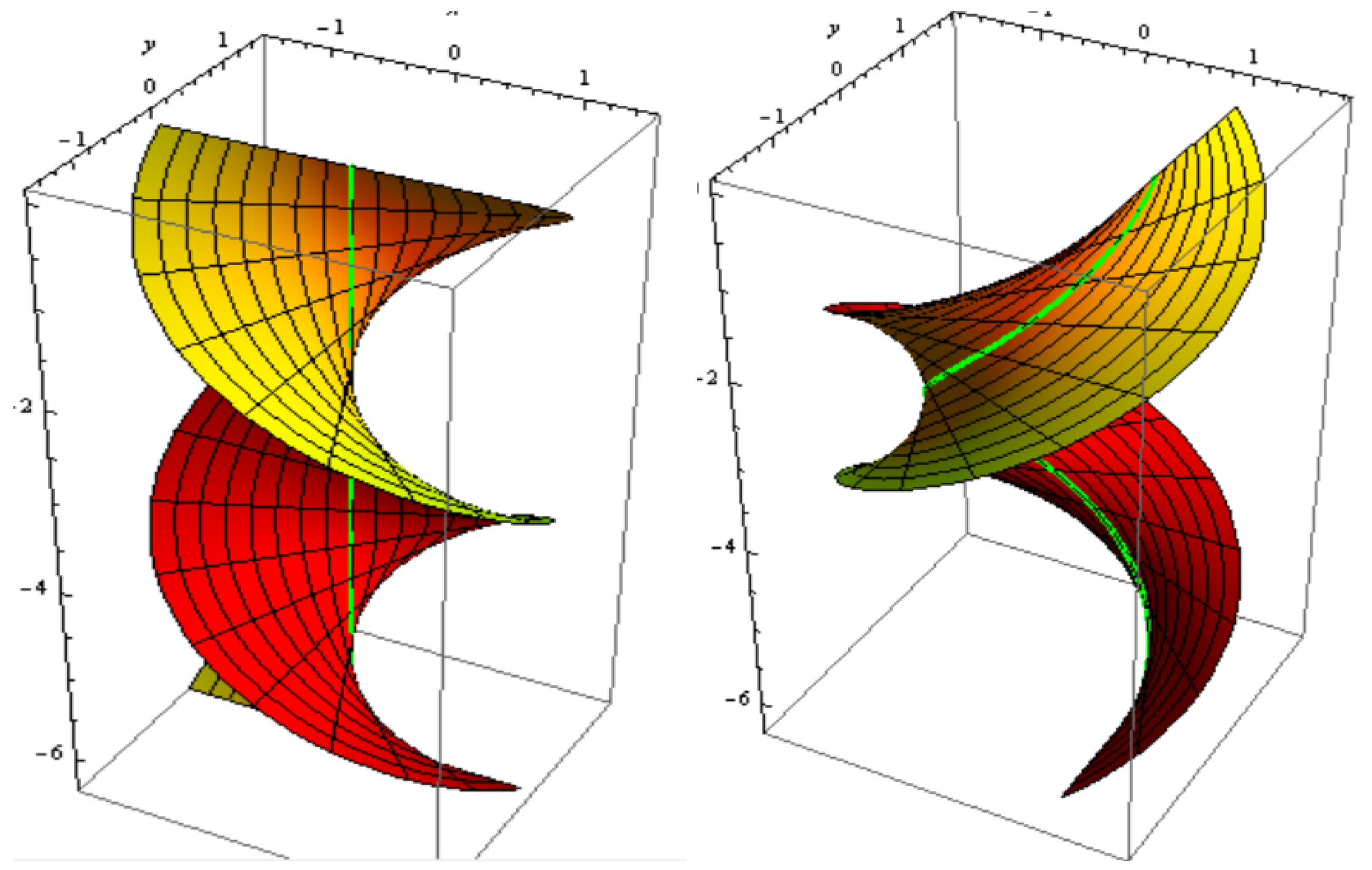
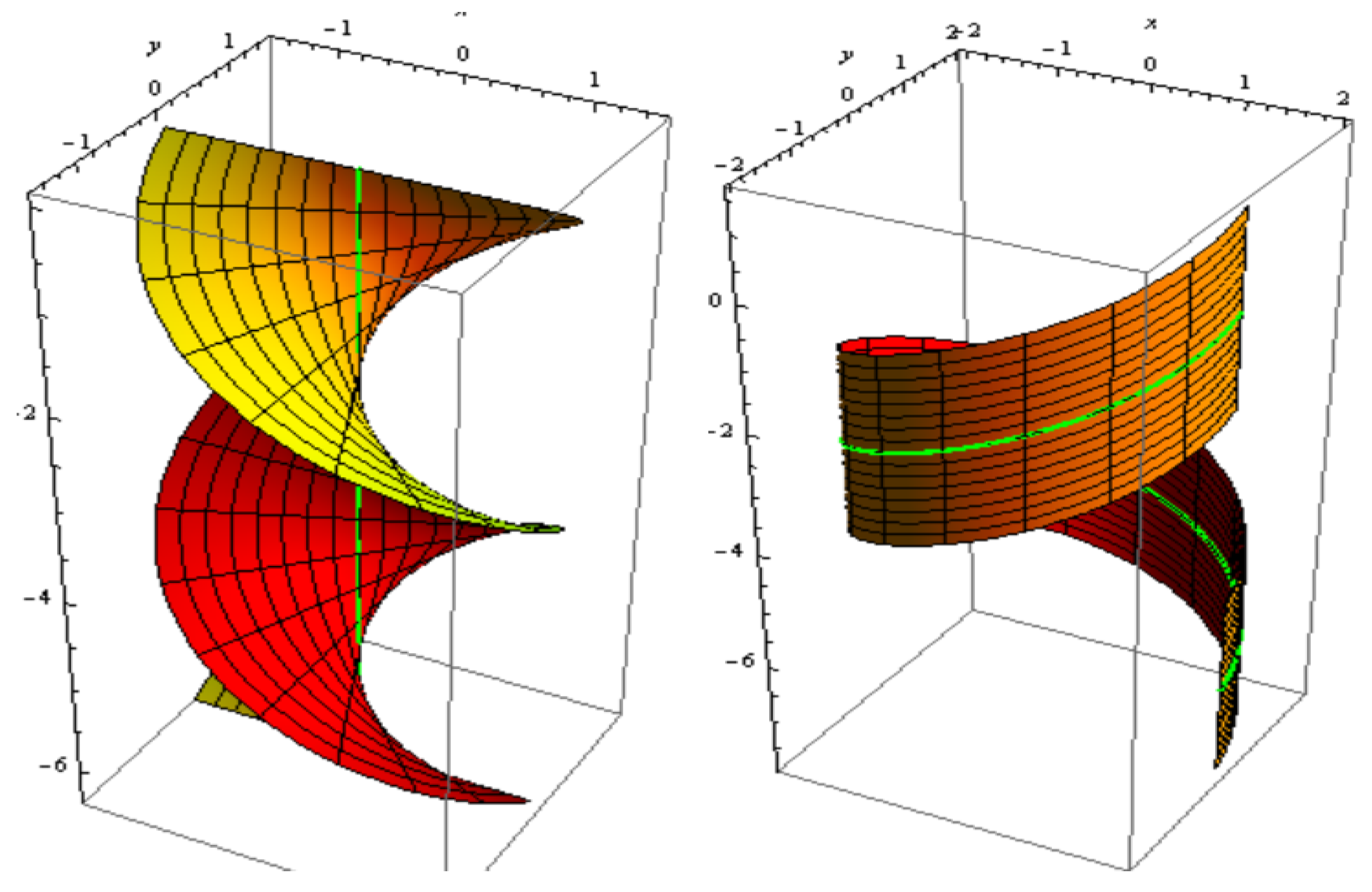
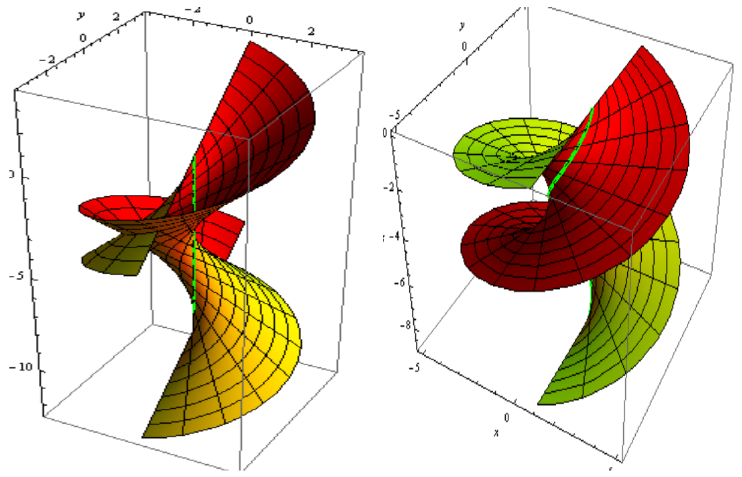
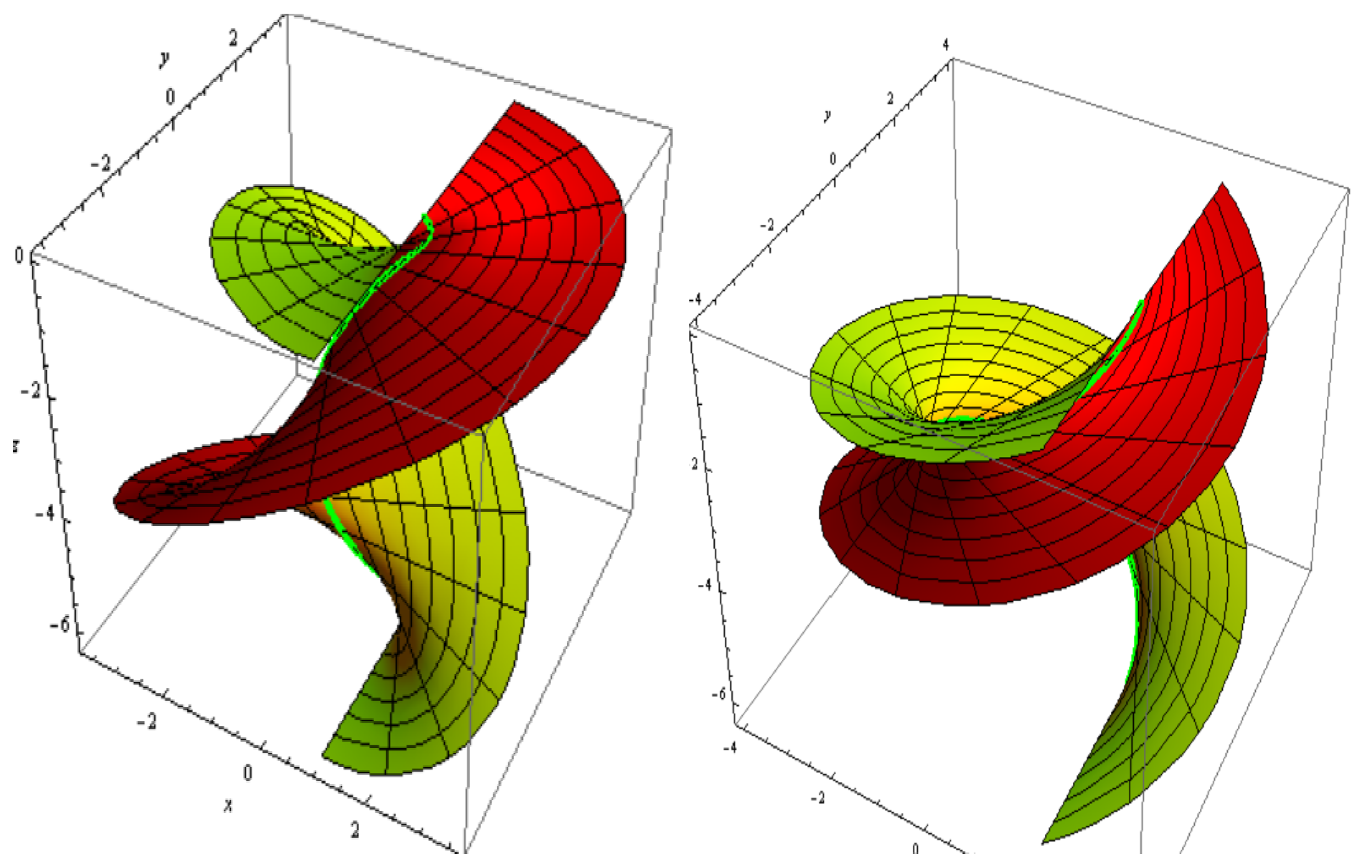
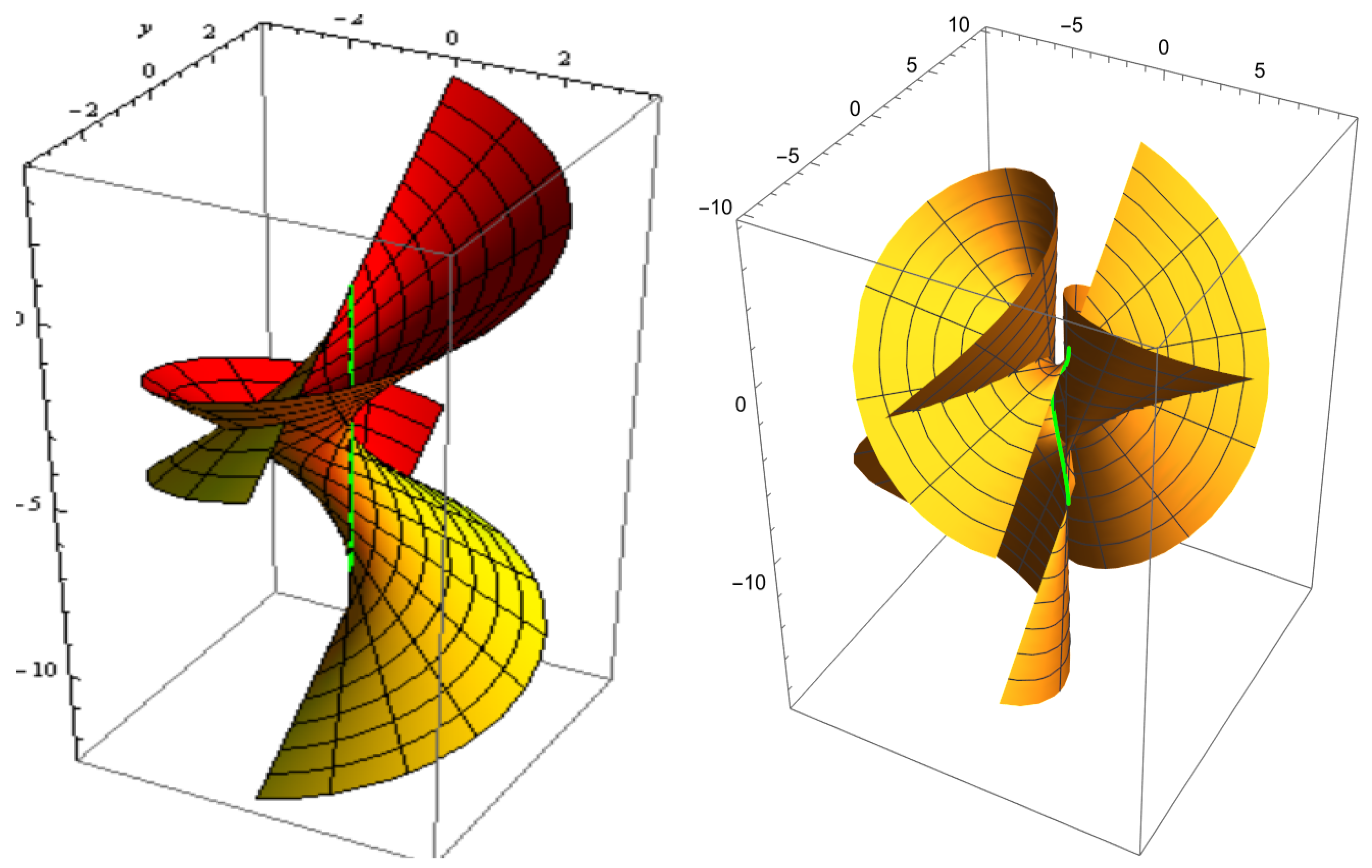
3.2. Construction of Slant Ruled Surface and Its $\mathcal{BO}$

In this subsection, we describe the construction of slant ruled surface and its $\mathcal{BO}$.

When $\chi \left(u\right)$ is stationary, from the Equations (2) and (7), we have the ODE, ${\mathfrak{e}}^{‴}+{\kappa }^2\mathfrak{e}=\mathbf{0}$. After numerous algebraic manipulations, the solution to this equation is

$$\mathfrak{e}\left(\phi \right)=\left(sin\alpha sin\phi ,sin\alpha cos\phi ,cos\alpha \right),$$

(25)

where $\phi =\sqrt{1+{\gamma }^2}u$. Thus, we immediately find that

$$\left.\begin{array}{c}\mathfrak{t}\left(\phi \right)=\frac{d\mathfrak{e}}{d\phi }{∥\frac{d\mathfrak{e}}{d\phi }∥}^{-1}=\left(cos\phi ,-sin\phi ,0\right),\hfill \\ \\ \mathfrak{f}\left(\phi \right)=\mathfrak{e}\times \mathfrak{t}=\left(cos\alpha sin\phi ,cos\alpha cos\phi ,-sin\alpha \right).\hfill \end{array}\right\}$$

(26)

Therefore, based on Equations (3), (25) and (26), the $\mathcal{SC}$$\mathfrak{c}\left(\phi \right)$ is:

$$\mathfrak{c}\left(\phi \right)=\left(\begin{array}{c}(\stackrel{\phi }{\underset{0}{\int }}\lambda sin\phi d\phi )sin\alpha +(\stackrel{\phi }{\underset{0}{\int }}\mu sin\phi d\phi )cos\alpha \\ (\stackrel{\phi }{\underset{0}{\int }}\lambda cos\phi d\phi )sin\alpha +(\stackrel{\phi }{\underset{0}{\int }}\mu cos\phi d\phi )cos\alpha \\ \left(\stackrel{\phi }{\underset{0}{\int }}\lambda d\phi \right)cos\alpha -\left(\stackrel{\phi }{\underset{0}{\int }}\mu d\phi \right)sin\alpha \end{array}\right)$$

(27)

Based on Equations (4), (25)–(27) the slant ruled surface $\mathcal{M}$ has the form

$$\mathfrak{r}(\phi ,v)=\left(\begin{array}{c}(\stackrel{\phi }{\underset{0}{\int }}\lambda sin\phi d\phi )sin\alpha +(\stackrel{\phi }{\underset{0}{\int }}\mu sin\phi d\phi )cos\alpha +vsin\alpha sin\phi \\ (\stackrel{\phi }{\underset{0}{\int }}\lambda cos\phi d\phi )sin\alpha +(\stackrel{\phi }{\underset{0}{\int }}\mu cos\phi d\phi )cos\alpha +vsin\alpha cos\phi \\ \left(\stackrel{\phi }{\underset{0}{\int }}\lambda d\phi \right)cos\alpha -\left(\stackrel{\phi }{\underset{0}{\int }}\mu d\phi \right)sin\alpha +vcos\alpha \end{array}\right)$$

(28)

According to the Equations (15), (20) and (27) the $\mathcal{BO}$ surface ${\mathcal{M}}^{*}$ can be inferred as

$${\mathfrak{r}}^{*}(\phi ,v)=\left(\begin{array}{c}(\stackrel{\phi }{\underset{0}{\int }}\lambda sin\phi d\phi )sin\alpha +(\stackrel{\phi }{\underset{0}{\int }}\mu sin\phi d\phi )cos\alpha +{\varphi }^{*}cos\phi +vsin\Theta sin\phi \\ (\stackrel{\phi }{\underset{0}{\int }}\lambda cos\phi d\phi )sin\alpha +(\stackrel{\phi }{\underset{0}{\int }}\mu cos\phi d\phi )cos\alpha -{\varphi }^{*}sin\phi +vsin\Theta cos\phi \\ \left(\stackrel{\phi }{\underset{0}{\int }}\lambda d\phi \right)cos\alpha -\left(\stackrel{\phi }{\underset{0}{\int }}\mu d\phi \right)sin\alpha +vcos\Theta \end{array}\right),$$

(29)

where $\Theta =\alpha +\varphi$.

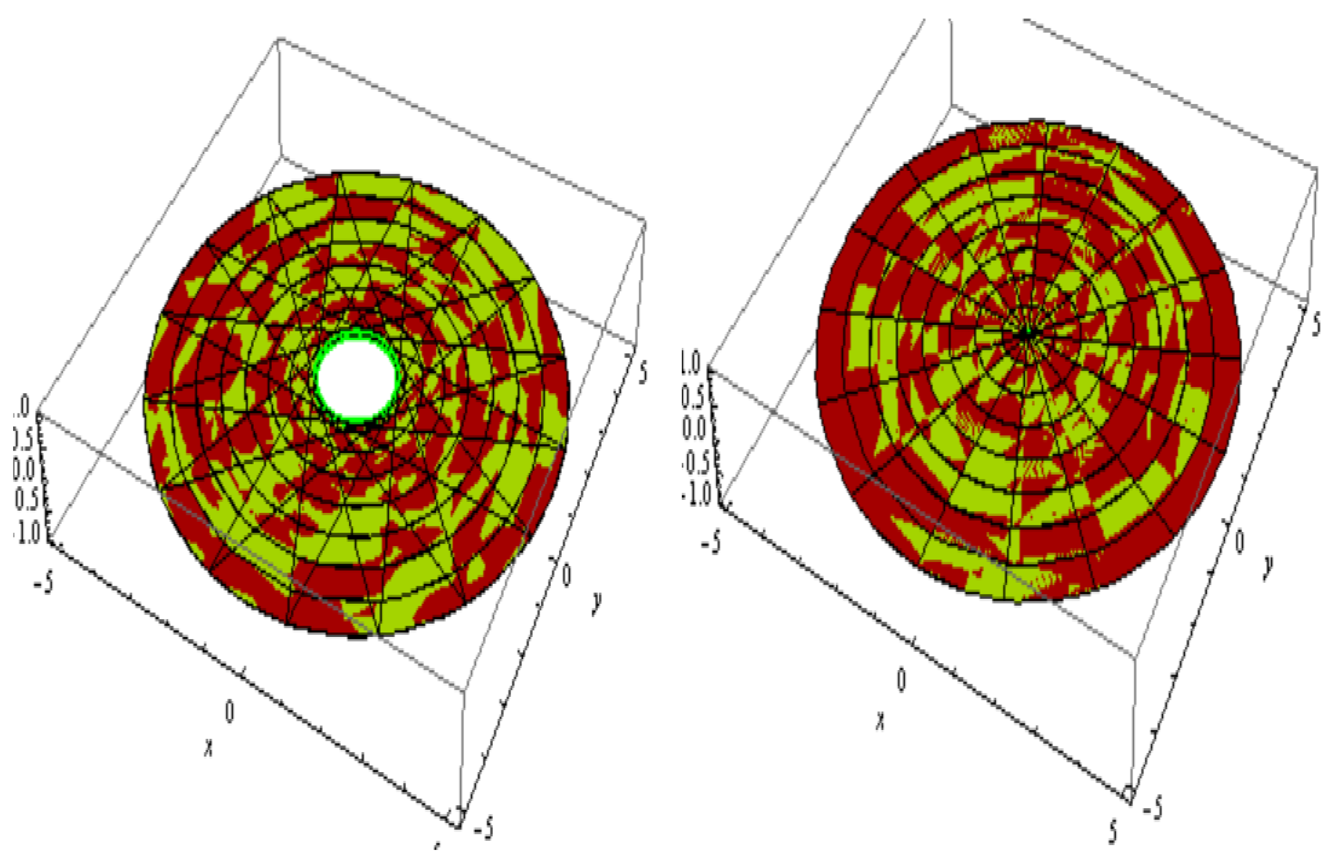
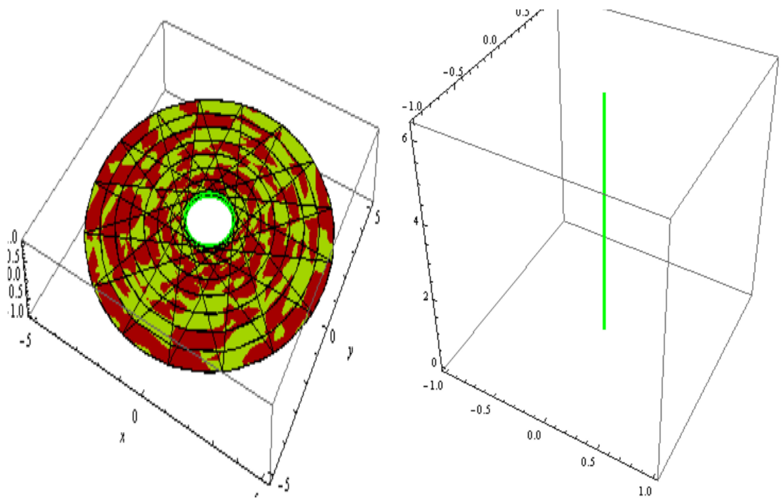
3.3. Classification of the Slant Ruled Surfaces

Based on the Equations (28) and (29), and via the shape of the striction curves, the slant $\mathcal{RS}$ and its $\mathcal{BO}$ can be classified into three kinds, as follows; we will consider ${\varphi }^{*}=1$.

Case 1. If the striction curve is an asymptotic curve, ${\kappa }_n=\lambda -\chi \mu =0$, there are two potential issues:

(a). In the issue of $\alpha =\pi /4$ ($\lambda =\mu )$, then we have

$$\mathfrak{r}(\phi ,v)=(\sqrt{2}\stackrel{\phi }{\underset{0}{\int }}\mu sin\phi d\phi +\frac{v}{\sqrt{2}}sin\phi ,\sqrt{2}\stackrel{\phi }{\underset{0}{\int }}\mu cos\phi d\phi +\frac{v}{\sqrt{2}}cos\phi ,\frac{v}{\sqrt{2}}),$$

and

$${\mathfrak{r}}^{*}(\phi ,v)=\left(\begin{array}{c}\sqrt{2}\stackrel{\phi }{\underset{0}{\int }}\mu sin\phi d\phi +cos\phi +\frac{v}{\sqrt{2}}(cos\varphi +sin\varphi )sin\phi \\ \sqrt{2}\stackrel{\phi }{\underset{0}{\int }}\mu cos\phi d\phi -sin\phi +\frac{v}{\sqrt{2}}(cos\varphi +sin\varphi )cos\phi \\ \frac{v}{\sqrt{2}}(cos\varphi -sin\varphi )\end{array}\right).$$

For $\mu \left(\phi \right)=\phi$, $-30\le$$v\le 30$, and $0\le$$\phi \le 2\pi$. The slant $\mathcal{RS}$ and its parallel offset are shown in Figure 1. The slant $\mathcal{RS}$ and its oriented offset are shown in Figure 2.

(b). In the issue of $\alpha =\pi /2$ ($\lambda =0)$, then we have

$$\mathfrak{r}(\phi ,v)=(vsin\phi ,vcos\phi ,-\stackrel{\phi }{\underset{0}{\int }}\mu d\phi ),$$

and

$${\mathfrak{r}}^{*}(\phi ,v)=(cos\phi +vcos\varphi sin\phi ,-sin\phi +vcos\varphi cos\phi ,-\stackrel{\phi }{\underset{0}{\int }}\mu d\phi -vsin\varphi )$$

For $\mu \left(\phi \right)=1$, $-1.5\le$$v\le 1.5$, and $0\le$$\phi \le 2\pi$, the slant $\mathcal{RS}$ and its parallel offset are shown in Figure 3. The slant $\mathcal{RS}$ and its oriented offset are shown in Figure 4.

Case 2. If the striction curve is a geodesic curve, we may write

$${\kappa }_g=\frac{1}{{\lambda }^2+{\mu }^2}\frac{d}{d\phi }(\mu \frac{d\lambda }{d\phi }-\lambda \frac{d\mu }{d\phi })=0\Rightarrow \lambda /\mu =c,$$

where c is an arbitrary constant. Thus, we may have two different cases:

(a). In the issue of $\alpha =\pi /4$, we have

$$\mathfrak{r}(\phi ,v)=\left(\begin{array}{c}\frac{c}{\sqrt{2}}(\stackrel{\phi }{\underset{0}{\int }}\mu sin\phi d\phi )+\frac{1}{\sqrt{2}}(\stackrel{\phi }{\underset{0}{\int }}\mu sin\phi d\phi )+\frac{v}{\sqrt{2}}sin\phi \\ \frac{c}{\sqrt{2}}(\stackrel{\phi }{\underset{0}{\int }}\mu cos\phi d\phi )+\frac{1}{\sqrt{2}}(\stackrel{\phi }{\underset{0}{\int }}\mu cos\phi d\phi )+\frac{v}{\sqrt{2}}cos\phi \\ \frac{c}{\sqrt{2}}(\stackrel{\phi }{\underset{0}{\int }}\mu d\phi )-\frac{1}{\sqrt{2}}(\stackrel{\phi }{\underset{0}{\int }}\mu d\phi )+\frac{v}{\sqrt{2}}\end{array}\right)$$

and

$${\mathfrak{r}}^{*}(\phi ,v)=\left(\begin{array}{c}\frac{c}{\sqrt{2}}\stackrel{\phi }{\underset{0}{\int }}\mu sin\phi d\phi +\frac{1}{\sqrt{2}}\stackrel{\phi }{\underset{0}{\int }}\mu sin\phi d\phi +cos\phi +vcos\varphi sin\phi \\ \frac{c}{\sqrt{2}}\stackrel{\phi }{\underset{0}{\int }}\mu cos\phi d\phi +\frac{1}{\sqrt{2}}\stackrel{\phi }{\underset{0}{\int }}\mu cos\phi d\phi -sin\phi +vcos\varphi cos\phi \\ \frac{c}{\sqrt{2}}\stackrel{\phi }{\underset{0}{\int }}\mu d\phi -\frac{1}{\sqrt{2}}\stackrel{\phi }{\underset{0}{\int }}\mu d\phi -vsin\varphi \end{array}\right).$$

For $\mu \left(\phi \right)=c=-1,$$-3\le$$v\le 3$, and $0\le$$\phi \le 2\pi$. The slant $\mathcal{RS}$ and its parallel offset are shown in Figure 5. The slant $\mathcal{RS}$ and its oriented offset are shown in Figure 6.

(b). For the issue of $\alpha =\pi /2$, we have

$$\mathfrak{r}(\phi ,v)=(c\stackrel{\phi }{\underset{0}{\int }}\mu sin\phi d\phi +vsin\phi ,\stackrel{\phi }{\underset{0}{c\int }}\mu cos\phi d\phi +vcos\phi ,-\stackrel{\phi }{\underset{0}{\int }}\mu d\phi ),$$

and

$${\mathfrak{r}}^{*}(\phi ,v)=\left(\begin{array}{c}c\stackrel{\phi }{\underset{0}{\int }}\mu sin\phi d\phi +cos\phi +vcos\varphi sin\phi \\ c\stackrel{\phi }{\underset{0}{\int }}\mu cos\phi d\phi -sin\phi +vcos\varphi cos\phi \\ -\stackrel{\phi }{\underset{0}{\int }}\mu d\phi -vsin\varphi \end{array}\right)$$

For $\mu \left(\phi \right)=-c=1,$$-1.5\le$$v\le 1.5$, and $0\le$$\phi \le 2\pi$. The slant $\mathcal{RS}$ and its parallel offset are shown Figure 7. The slant $\mathcal{RS}$ and its oriented offset are shown in Figure 8.

Case 3. If the striction curve is a curvature line, we may write $\mu +\chi \lambda =\mathfrak{0}$, and we may have two different cases:

(a). In the issue of $\alpha =\pi /4$ ($\lambda =-\mu )$, then we have

$$\mathfrak{r}(\phi ,v)=(\frac{v}{\sqrt{2}}sin\phi ,\frac{v}{\sqrt{2}}cos\phi ,-\sqrt{2}\stackrel{\phi }{\underset{0}{\int }}\mu d\phi +\frac{v}{\sqrt{2}}),$$

and

$${\mathfrak{r}}^{*}(\phi ,v)=(cos\phi +vcos\varphi sin\phi ,-sin\phi +vcos\varphi cos\phi ,-\sqrt{2}\stackrel{\phi }{\underset{0}{\int }}\mu d\phi -vsin\varphi ).$$

For $\mu \left(\phi \right)=1,$$-2\le$$v\le 2$, and $0\le$$\phi \le 2\pi$. The slant $\mathcal{RS}$ and its parallel offset are shown in Figure 9. The slant $\mathcal{RS}$ and its oriented offset are shown in Figure 10.

(b). For the issue of $\alpha =\pi /2$ ($\mu =0)$, we have

$$\mathfrak{r}(\phi ,v)=(\stackrel{\phi }{\underset{0}{\int }}\lambda sin\phi d\phi +vsin\phi ,\stackrel{\phi }{\underset{0}{\int }}\lambda cos\phi d\phi +vcos\phi ,0),$$

and

$${\mathfrak{r}}^{*}(\phi ,v)=\left(\begin{array}{c}\stackrel{\phi }{\underset{0}{\int }}\lambda sin\phi d\phi +cos\phi +vcos\varphi sin\phi \\ \stackrel{\phi }{\underset{0}{\int }}\lambda cos\phi d\phi -sin\phi +vcos\varphi cos\phi \\ -vsin\varphi \end{array}\right)$$

(30)

For $\lambda \left(\phi \right)=1,$$-2\le$$v\le 2$, and $0\le$$\phi \le 2\pi$. The slant $\mathcal{RS}$ and its parallel offset are shown in Figure 11. The slant $\mathcal{RS}$ and its oriented offset are shown in Figure 12.

4. Conclusions

This paper develops a theory regarding $\mathcal{BO}$ of slant ruled surfaces analogous to the slant curve theory. In this paper, we legalize the general parameterization of a slant ruled surface in the Euclidean 3-space ${\mathcal{E}}^3$. In terms of this, we discuss the properties of the position vectors of the $\mathcal{BO}$ for slant ruled and developable surfaces. Hopefully, these scores will be useful in the field of model-based manufacturing of mechanical products, as well as in geometric modeling. The authors plan to apply this work in diverse spaces and discuss the categorization of singularities as they are pointed out in [26,27].

References

1. Gugenheimer, H.W. Differential Geometry; Graw-Hill: New York, NY, USA, 1956; pp. 162–169. [Google Scholar]
2. Bottema, O.; Roth, B. Theoretical Kinematics; North-Holland Press: New York, NY, USA, 1979. [Google Scholar]
3. Karger, A.; Novak, J. Space Kinematics and Lie Groups; Gordon and Breach Science Publishers: New York, NY, USA, 1985. [Google Scholar]
4. Papaionnou, S.G.; Kiritsis, D. An application of Bertrand curves and surfaces to CAD/CAM. Comput. Aided Des. 1985, 17, 348–352. [Google Scholar] [CrossRef]
5. Schaaf, J.A. Geometric Continuity of Ruled Surfaces. Comput. Aided Geom. Des. 1998, 15, 289–310. [Google Scholar] [CrossRef]
6. Peternell, M.; Pottmann, H.; Ravani, B. On the computational geometry of ruled surfaces. Comput.-Aided Des. 1999, 31, 17–32. [Google Scholar] [CrossRef]
7. Pottman, H.; Wallner, J. Computational Line Geometry; Springer: Berlin/Heidelberg, Germany, 2001. [Google Scholar]
8. Ravani, B.; Ku, T.S. Bertrand offsets of ruled and developable surfaces. Comput. Aided Des. 1991, 23, 145–152. [Google Scholar] [CrossRef]
9. Küçük, A.; Gürsoy, O. On the invariants of Bertrand trajectory surface offsets. AMC 2003, 11–23. [Google Scholar] [CrossRef]
10. Kasap, E.; Kuruoglu, N. Integral invariants of the pairs of the Bertrand ruled surface. Bull. Pure Appl. Sci. Sect. E Math. 2002, 21, 37–44. [Google Scholar]
11. Kasap, E.; Kuruoglu, N. The Bertrand offsets of ruled surfaces in R 1 3 . Acta Math. Vietnam. 2006, 31, 39–48. [Google Scholar]
12. Kasap, E.; Yuce, S.; Kuruoglu, N. The involute×-evolute offsets of ruled surfaces. Iran. J. Sci. Tech. Trans. A 2009, 33, 195–201. [Google Scholar]
13. Orbay, K.; Kasap, E.; Aydemir, I. Mannheim offsets of ruled surfaces. Math Probl. Eng. 2009, 2019, 160917. [Google Scholar] [CrossRef]
14. Onder, M.; Ugurlu, H.H. Frenet frames and invariants of timelike ruled surfaces. Ain. Shams Eng. J 2013, 4, 507–513. [Google Scholar] [CrossRef]
15. Sentrk, G.Y.; Yuce, S. Properties of integral invariants of the involute-evolute offsets of ruled surfaces. Int. J. Pure Appl. Math. 2015, 102, 757–768. [Google Scholar] [CrossRef]
16. Yoon, D.W. On the evolute offsets of ruled surfaces in Minkowski 3-space. Turk. J. Math. 2016, 40, 594–604. [Google Scholar] [CrossRef]
17. Onder, M. Non-Null slant ruled surfaces. Aims Math. 2019, 4, 384–396. [Google Scholar] [CrossRef]
18. Onder, M.; Kaya, O. Characterizations of slant ruled surfaces in the Euclidean 3-space. Casp. J. Math. Sci. 2017, 6, 31–46. [Google Scholar]
19. Aldossary, M.T.; Abdel-Baky, R.A. On the Blaschke approach of Bertrand offsets of spacelike ruled surfaces. AIMS Math. 2022, 6, 3339–3351. [Google Scholar] [CrossRef]
20. Alluhaibi, N.; Abdel-Baky, R.A.; Naghi, M. On the Bertrand Offsets of Timelike Ruled Surfaces in Minkowski 3-Space. Symmetry 2022, 4, 673. [Google Scholar] [CrossRef]
21. Nazra, S.; Abdel-Baky, R.A. Bertrand offsets of ruled surfaces with Blaschke frame in Euclidean 3-space. Axioms 2023, 12, 649. [Google Scholar] [CrossRef]
22. Mofarreh, F.; Abdel-Baky, R.A. Surface pencil pair interpolating Bertrand pair as common asymptotic curves in Euclidean 3-space. Mathematics 2023, 11, 3495. [Google Scholar] [CrossRef]
23. Şentürk, G.Y.; Salim, Y. Bertrand offsets of ruled surfaces with Darboux frame. Results Math. 2016, 72, 1151–1159. [Google Scholar] [CrossRef]
24. Şentürk, G.Y.; Salim, Y. On the evolute offsets of ruled surfaces using the Darboux frame. Commun. Fac. Sci. Univ. Ank. Ser. A1 Math. Stat. 2019, 68, 1256–1264. [Google Scholar] [CrossRef]
25. Bruce, J.W.; Giblin, P.J. Curves and Singularities, 2nd ed.; Cambridge University Press: Cambridge, UK, 1992. [Google Scholar]
26. Almoneef, A.; Abdel-Baky, R.A. Singularity properties of spacelike circular surfaces. Symmetry 2023, 15, 842. [Google Scholar] [CrossRef]
27. Nazra, S.; Abdel-Baky, R.A. Singularities of non-lightlike developable surfaces in Minkowski 3-space. Mediterr. J. Math. 2023, 20, 45. [Google Scholar] [CrossRef]
Figure 1. Slant RS (left) and its parallel offset (right).
Symmetry 16 00235 g001
Figure 2. Slant RS (left) and its oriented offset (right).
Symmetry 16 00235 g002
Figure 3. Slant ruled surface (left) and its oriented offset (right).
Symmetry 16 00235 g003
Figure 4. Slant RS (left) and its parallel offset (right).
Symmetry 16 00235 g004
Figure 5. Slant RS (left) and its parallel offset (right).
Symmetry 16 00235 g005
Figure 6. Slant RS (left) and its oriented offset (right).
Symmetry 16 00235 g006
Figure 7. Slant RS (left) and its parallel offset (right).
Symmetry 16 00235 g007
Figure 8. Slant RS (left) and its oriented offset (right).
Symmetry 16 00235 g008
Figure 9. Slant RS (left) and its parallel offset (right).
Symmetry 16 00235 g009
Figure 10. Slant RS (left) and its oriented offset (right).
Symmetry 16 00235 g010
Figure 11. Slant RS (left) and its parallel offset (right).
Symmetry 16 00235 g011
Figure 12. Slant RS (left) and its oriented offset (right).
Symmetry 16 00235 g012
Disclaimer/Publisher’s Note: The statements, opinions and data contained in all publications are solely those of the individual author(s) and contributor(s) and not of MDPI and/or the editor(s). MDPI and/or the editor(s) disclaim responsibility for any injury to people or property resulting from any ideas, methods, instructions or products referred to in the content.