Article

How the Magnetization Angle of a Linear Halbach Array Influences Particle Steering in Magnetic Drug Targeting—A Systematic Evaluation and Optimization

Institute for Electronics Engineering, Friedrich-Alexander-Universität Erlangen-Nürnberg, Cauerstr. 9, 91058 Erlangen, Germany
*
Author to whom correspondence should be addressed.
Symmetry 2024, 16(2), 148; https://doi.org/10.3390/sym16020148
Submission received: 18 December 2023 / Revised: 15 January 2024 / Accepted: 17 January 2024 / Published: 26 January 2024
(This article belongs to the Section Mathematics)

Abstract

:
The main challenge in magnetic drug targeting lies in steering the magnetic particles, especially in deeper body layers. For this purpose, linear Halbach arrays are currently in focus. However, to the best of the authors’ knowledge, the impact of the magnetization angle between two neighboring magnets in Halbach arrays has not been investigated for particle steering so far. Therefore, in this paper, a systematic numerical parameter study of varying the magnetization angle of linear Halbach arrays is conducted. This is completed by undertaking a typical magnetic drug targeting scenario, where magnetic particles have to be steered in an optimized manner. This includes the calculation of the magnetic flux density, its gradient, the total magnetic energy, and the resulting magnetic force based on a fitting function for the different Halbach constellations in the context of examining their potential for predicting the particle distribution. In general, increased magnetization angles result in an increased effective range of the magnetic force. However, as there is a trade-off between a weak force on the weak side of the array and a simple manufacturing process, a magnetization angle of 90 is recommended. For evaluating the steering performance, a numerical or experimental evaluation of the particle distribution is mandatory.

1. Introduction

The interest in steering, separating, or trapping magnetic nanoparticles or cells, especially in biological and medical applications, has grown rapidly in recent decades [1,2,3,4]. One of these applications is so-called magnetic drug targeting (MDT) in cancer therapy [5]. This method is based on superparamagnetic iron oxide nanoparticles (SPIONs) as carriers to which the anticancer agents are attached. These SPIONs are injected into the vascular system and conveyed by the blood flow to the targeted region due to the influence of an external applied magnetic field [6]. In the case of lung cancer, the SPIONs are inhaled [7]. MDT considerably decreases the overall dose and side effects on healthy tissues since SPIONs coated with drugs are concentrated in the targeted region and maintained there due to a holding magnetic field [8]. In other words, MDT improves the efficiency of cancer therapy as it has a local cancer treatment effect [9,10]. Moreover, it reduces unwanted adverse effects, which was experimentally proven in 2013 by Tietze et al. [11]. A typical MDT scenario and its modelling are illustrated in Figure 1. An extensive review of MDT approaches, release control of the particles, and an overview of the existing clinical studies are provided by Ulbrich et al. [12]. The drug is released at the tumor region over time, or an alternating magnetic field is applied to the particles, resulting in heating, which is known as hyperthermia [13]. However, the success of such a treatment depends on the number of SPIONs reaching the tumor and being trapped there. For this purpose, most researchers think of placing permanent magnets [14,15] or electromagnets [16,17,18] outside the body. Since the usable reach of the magnetic field and especially of the magnetic force is a significant problem [19], it is also being considered to place the patient inside a magnetic resonance imaging (MRI) scanner [20], offering a strong constant field plus switchable overlay fields, or even implanting permanent magnets next to the tumor region [21,22].
No matter the specific magnetic field design, there is always a trade-off between too strong a magnetic field, which causes all SPIONs to stick to the vessel wall, or a magnetic field that is too weak to attract the SPIONs [15]. Figure 2 illustrates that, due to the background velocity flow field, the particles in the upper half of the vessel automatically take the correct outlet in a symmetrical bifurcation. Thus, the particles injected in the lower half of the vessel must be pulled into the upper part while simultaneously preventing the particles already in the upper part to become accumulated and remain stuck at the vessel wall. As the magnetic field approximately decays with the cubic distance R 3 [23], this worsens steering performance since the magnetic force is stronger closer to the magnet. Moreover, accumulated particles show a shielding behavior, reducing the magnetic forces [24].
To overcome this problem, many researchers use electromagnets (EMs) on two sides of a tube, which are alternately switched on and off to steer particles through a bifurcation [25,26,27] and optimize the switching algorithm by defining safety zones [28,29,30,31]. Moreover, Le et al. [32] used four EMs to generate a focused field-free point that can be shifted in place to avoid stuck particles at the vessel wall. However, EMs require an additional power supply in the kW range, with currents greater than 200 A inducing heat, therefore requiring additional cooling [33]. On the other hand, rare earth permanent magnets (PMs), like NdFeB, generate a low-cost and strong magnetic field. Thus, they are studied for attracting or steering magnetic nanoparticles too [15,34,35]. However, permanent magnets have the disadvantage that their magnetic field can only be changed by mechanical operations (e.g., rotating or changing the position). Thus, Surpi et al. [36] investigated the behavior of SPIONs under two moving PMs placed on opposite sides of a tube, and Baun et al. [37] precisely steered SPIONs in a static fluid with a cylindrical array of PMs surrounding the particle container. A more detailed review of the current state-of-the-art publications for steering magnetic nanoparticles in an MDT scenario is provided and discussion in Section 5.4.
Nevertheless, the accumulation of the SPIONs in the tumor and, thus, the efficiency of an MDT treatment depend on numerous parameters, like the flow of blood with the corresponding geometry of the vessel and tumor, the properties of the SPIONs, as well as the gradient of the magnetic field [3,38]. As we cannot adjust the blood flow and the nanoparticles have to have a diameter <200 nm to not be recognized by the body’s immune system and be able to penetrate into tissue [39], only the magnetic field can be appropriately designed. Here, a strong gradient field over a large distance is mandatory [38,40]. However, our previous study showed that, for the same magnetic effort, a longer magnetic array with a lower absolute magnetic field strength leads to the same particle attraction as a shorter array with a higher field strength [41].
In the literature, different types of arrays, mostly entirely consisting of PMs [42,43] but also of EMs [44], as well as hybrid ones [45,46], are discussed. The arrays are arranged linearly and parallel to the vessel [47] as well as coaxial structures surrounding the vessel [37]. As in medical applications placing the magnets surrounding the vessel is not possible, this paper will focus on linear arrays. In most of the literature, the magnets are arranged as a Halbach array [19], which is a promising structure since its pattern produces the strongest magnetic flux density [48]. Kang et al. [49] showed that the attraction force of a Halbach structure is stronger than when the single magnets are magnetized in alternating directions. Häfeli et al. [50] compared different array shapes and also concluded that Halbach arrays have the best particle trapping close to a surface. However, in [50], a Halbach structure with a shifted magnetization direction of 45 ° between two neighboring magnets was investigated. In our previous publication [51], we demonstrated that the attraction force is even higher when the neighboring magnets have a shifted magnetization of 90 ° . Also, in most of the literature, 90 ° is used for steering or attracting magnetic nanoparticles [47,49,52,53,54]. In other applications of Halbach arrays, various magnetization angles are investigated and discussed, e.g., 45 ° by Zhang et al. [55], 30 ° by Di Gerlando et al. [56], 18 ° and 22.5 ° by Shen et al. [57], and 90 ° by Li et al. [58].
To the best of the authors’ knowledge, the optimal magnetization angle between two adjacent magnets in a Halbach array for the application of attracting magnetic nanoparticles has not been systematically analyzed so far. With this paper, we want to close this gap in the state of the art. Our key contributions are summarized:
  • We systematically numerically investigate the impact of the magnetization angle in a reduced complexity 2D simulation in COMSOL Multiphysics® 6.1 regarding the steering performance of SPIONs in a background flow through a Y-shaped bifurcation.
  • We further evaluate the magnetic force for the strong and weak side of the array for different magnetization angles at its strongest position. We additionally compare the magnitude of the magnetic forces with the hydrodynamic drag force.
  • Since the calculation of the magnetic gradient leads to huge errors due to the discrete mesh in COMSOL, it was determined analytically using an exponential fitting function similar to [51]. By doing so, we further analyze if the magnetic flux density can be approximated with an exponential function for other magnetization angles too.
  • Since we were not able to identify standardized evaluation parameters with our comprehensive analysis of the state of the art (compare Section 5.4), the significance of various evaluation parameters, such as the magnetic field, total applied magnetic energy, or maximum gradient in the vessel, is examined regarding their prediction of particle steering.
  • Based on our investigations, recommendations for the design of a linear Halbach array for steering SPIONs in MDT are derived and discussed.
Our paper is structured as follows: after the introduction in Section 1, the fundamentals and physical background of SPIONs, (linear) Halbach arrays, and their magnetic flux density are provided in Section 2. In Section 3, the simulation model is defined, and the evaluation process of this study is introduced. Afterwards, the results are presented in Section 4. Finally, in Section 5, the results are discussed regarding particle steering, including the strength and usable range of the magnetic field and force. Furthermore, recommendations for the design of a linear Halbach array are provided and the results of this paper are compared with the state of the art of particle steering in an MDT scenario. Moreover, the limitations of this study are identified. The paper is concluded in Section 6 and an outlook of future steps is provided.

2. Fundamentals and Background

2.1. Superparamagnetic Iron Oxide Nanoparticles

In MDT, superparamagnetic iron oxide nanoparticles (SPIONs) with a diameter of <250 nm are usually used as carriers for cancer drugs [39,59]. The SPIONs are coated, e.g., by lauric acid layers, to be biocompatible [60] and stable in blood [39]. Furthermore, they can be synthesized small enough not to be attacked by the body’s immune system [6,61].
Superparamagnetism exists in small ferromagnetic particles [62]. These particles consist only of single-domain magnetization, which flips randomly in time, resulting in an average magnetization to be zero [39,62]. Therefore, SPIONs have strong magnetization with no hysteretic behavior, and, consequently, the particles do not accumulate [61]. This is advantageous for medical applications since the risk of obstructing blood vessels is reduced. Lunnoo et al. [63] analyzed the size-dependent capture efficiency of SPIONs by a magnet at a desired location depending on magnetic cores made from different materials, such as Fe3O4, Fe2O3, and Fe nanoparticles with different coating layers, such as Au, PEG, and SiO2. They focused on particle sizes ranging from 10 nm to 200 nm, which is seen as optimal for in vivo delivery [6]. Their results showed that larger particles had better capture efficiency than smaller particles. This is reasonable as the magnetic force is directly proportional to the volume of the particles [40]. The material of magnetic cores and coating layers did not significantly influence the capture efficiency.

2.2. Forces on SPIONs

Using Ampere’s law × H = J in the quasi-static case, and magnetostatic field dependencies B = × A , the equation of the magnetic field can be described as [64]
× ( 1 μ 0 × A M ) = 0 .
Here, μ 0 = 4 π · 10 7 H/m corresponds to the permeability of the free space, A is the magnetic vector potential (Vs/m), and M is the volume magnetization vector (A/m). Furthermore, J is the current density (A/m2), B is the magnetic flux density (T), and H is the magnetic field strength (A/m).
The theory of magnetic flux conservation in the human body can be represented using the relation between B and H :
B = μ 0 μ r H blood , tissue , and air μ 0 ( H + M ) PM
Here, μ r describes the relative permeability of a medium. For example, for blood and air, μ r is approximately 1 [65]. Aside from the magnetic field, the blood flow and properties of SPIONs also play an essential role in the performance of particle steering. To determine the velocity field and the pressure distribution of the background flow, the equation of mass and the Navier–Stokes equation for a Newtonian and incompressible fluid are used [63,66]
ρ · u = 0 ,
ρ ( u · u ) = p + η · ( u ) + F .
Thereby, ρ corresponds to the mass density of the background flow (kg/m3), u is the velocity vector (m/s), p is pressure (Pa), η is the fluid’s viscosity (Pa·s), and F is the external volume force (N/m3). For the sake of simplicity, in this paper, the medium of the background flow is assumed to be water since the flow properties of blood are much more complex. The interested reader can find detailed information regarding the mathematical modeling of magnetic nanoparticles in a blood flow for MDT in the work of Fanelli et al. [67].
To represent the particle tracing process, Newton’s second law is used to describe the balance of forces on one SPION [66]
F p = d ( m p u p ) d t ,
where m p corresponds to the mass of the particle (kg), and u p is the velocity of the particle (m/s). F p is a force acting on the particle (N).
As the SPIONs are small in size, when one SPION is moving through the blood vessel, it mainly experiences two forces, namely the magnetophoretic force F m and the hydrodynamic drag force F d [3,68,69]. Other forces such as gravitational force F g , buoyancy force F b , and lift force F l can be neglected because they are significantly weaker compared to F m and F d in MDT [3,66,70]. As a result, Equation (5) can be rewritten as
F m + F d = d ( m p u p ) d t .
The hydrodynamic drag force is also called the viscous drag force or only drag force [71]. This force describes the resistance when a spherical particle is moving through viscous fluid. For low-flow regimes with low Reynolds numbers Re, a laminar flow with a parabolic flow profile is obtained [3,72]. According to Stokes’ law, F d is calculated as [27,37]
F d = 6 π η R H ( u p u b ) ,
where R H is the hydrodynamic radius of the particle (m), η corresponds to the dynamic viscosity of the fluid medium (Pa·s), and u b and u p are the velocity of the background fluid (m/s) and the particle (m/s), respectively. For sake of simplicity, in this paper, the hydrodynamic radius R H of one SPION is set to be equal to the magnetic radius of the particle R p . In MDT, the magnitude of | F d | is in the range of 10 14 to 10 7 N and the velocity of blood 0.5 mm/s to 40 cm/s, respectively [1].
In general, on a microscopic scale and for a constant temperature, the magnetic force F m acting on a magnetic material at a certain position r is defined by [23,37]
F m r = m r · B ,
with the magnetic flux density B acting on a material of the magnetic moment m ( A · m 2 ). As the magnetic moment m inside one SPION aligns parallel to B , the magnetic force can also expressed as
F m r = m r · B = m · B .
Moreover, Equation (8) can be rewritten as [40]
F m = m · B = B · m + m · B + B × × m + m × × B .
For SPIONs, the magnetic moment m is usually assigned to be homogeneous (no spatial dependency) within one SPION. This leads to B · m = 0 . In [40], it was stated that, for particle steering, the SPIONs can be assumed to be magnetic dipoles. This cancels × m = 0 because m is not a function of B r . As in this paper, permanent magnets are used as magnetic field sources; the current density J is equal to zero. This results in × B = 0 . Thus, F m can be written as
F m = m · B ,
which is also known as Kelvin force [40]. The magnetic moment m can be deduced from the integral of the magnetization M (A/m) over the corresponding volume V ( m 3 ) [23]. For SPIONs, the magnetization is usually assigned to be homogeneous within one SPION and provided by
M = M sat · L m · B k T ,
where M sat corresponds to the saturation magnetization (A/m), k 1.3806 · 10 23 J/K is the Boltzmann constant, and T (K) the absolute temperature [73,74]. Moreover, L is the Langevin function, which has a strictly monotonously increasing behavior.
If the magnetic force is acting on microscale entities, it is called magnetophoretic force [3,75]. By solving the magneto-static boundary value problem for one spherical particle, the magnetophoretic force F m can be formulated as [23,69]
F m = 2 π μ b R p 3 μ p μ b μ p + 2 μ b | H | 2 .
Thereby, μ b and μ p are the magnetic permeability of the background medium and the particle, respectively. Moreover, R p is the radius of the particle and H is the gradient of the magnetic field excitation. Assuming a homogeneous magnetization within one SPION that is aligned parallel to the applied magnetic field, and based on Equation (11), the magnitude of the magnetophoretic force | F m | can be simplified to [51]
| F m | = | m · B | = m | B | = V p M | B | .
Thus, | F m | only depends on the SPION’s volume V p , the magnetization M, and the gradient of the magnetic flux density B . In the application of MDT, the magnitude | F m | can obtain values from 10 25 to 10 11 N, depending especially on B [1].
In MDT, F m and F d can usually be assumed to be perpendicular (compare Figure 2). Since F d is determined by the velocity flow of the blood, which is not adjustable, F m has to be maximized, which is the case for a Halbach arrangement.

2.3. Linear Halbach Array

A Halbach array is a special magnetic array in which the array’s single magnets are arranged so that the magnetic flux density is destructively and constructively superimposed on opposite sides of the array [76,77]. An illustration of a linear Halbach array arrangement is depicted in Figure 3. The magnetization pattern results in the ideal case in a one-sided magnetic field. Kang et al. [49] showed that the magnetic flux density and its gradient on the strong side of the array and, therefore, the magnetic force are stronger compared to a pattern where the magnetization direction of the single magnets point in alternating directions.
Halbach arrays were proposed by K. Halbach in 1980 for focusing charged particles in accelerator beams [77,78]. However, these arrays are found in the current literature mainly for shaping the fields of electric motors [79,80,81], but also in other various applications such as energy harvesting [82], induction-based cooking [83], refrigerators [84], or in medical applications such as magnetic resonance imaging (MRI) [85] or just as well in MDT [19].
For particle steering, most Halbach arrangements are linear and consist entirely of PMs (e.g., [43,47,49,51,52,54]). However, there are also 3D Halbach arrays consisting of EMs [86], which are combined with a core to focus SPIONs at a desired location (usually the tumor), or 3D constructs [37,87], which enclose the vessel and can precisely steer SPIONs here. However, since it is impossible to place the magnets around the blood vessel in reality, this paper focuses on linear arrays placed sideways to a vessel. The pattern of a linear Halbach array with a magnetization angle ϑ = 90 between two neighboring magnets is depicted in Figure 3. Hilton et al. [88] analyzed the torque ( N · m ) τ = m × B [23] of a Halbach array, as depicted in Figure 3, and figured out that, for a practical implementation, mechanical stabilization is crucial. Moreover, our paper also investigates other Halbach array patterns with varying magnetization angles between two neighboring magnets. An overview of different investigated array patterns is provided in Figure 4.

2.4. Magnetic Flux Density of a Linear Halbach Array

According to the literature, a Halbach array’s magnetic flux density B is computed with numerical methods or programs like COMSOL Multiphysics® 6.1 [88,89]. Nevertheless, in our previous paper [51], we showed that the magnitude of the magnetic flux density perpendicular to a linear Halbach array with a magnetization angle of ϑ = 90 can be approximated with an exponential function
B = ^ k 1 e k 2 y .
For an array with N = 8 magnets, this exponential approach describes B with a relative error of approximately 3.85% [51]. In Equation (15), k 1 and k 2 correspond to arbitrary fitting constants, which can be determined using a least square (LS) algorithm. In the scope of this paper, we want to investigate if the magnetic flux density of the Halbach array can also be approximated for other magnetization angles by this exponential function. Thus, the constants k 1 and k 2 are fitted based on the simulation results for both the strong and the weak side of the Halbach array for varying magnetization angles.

3. Definition of Simulation Model and Data Evaluation

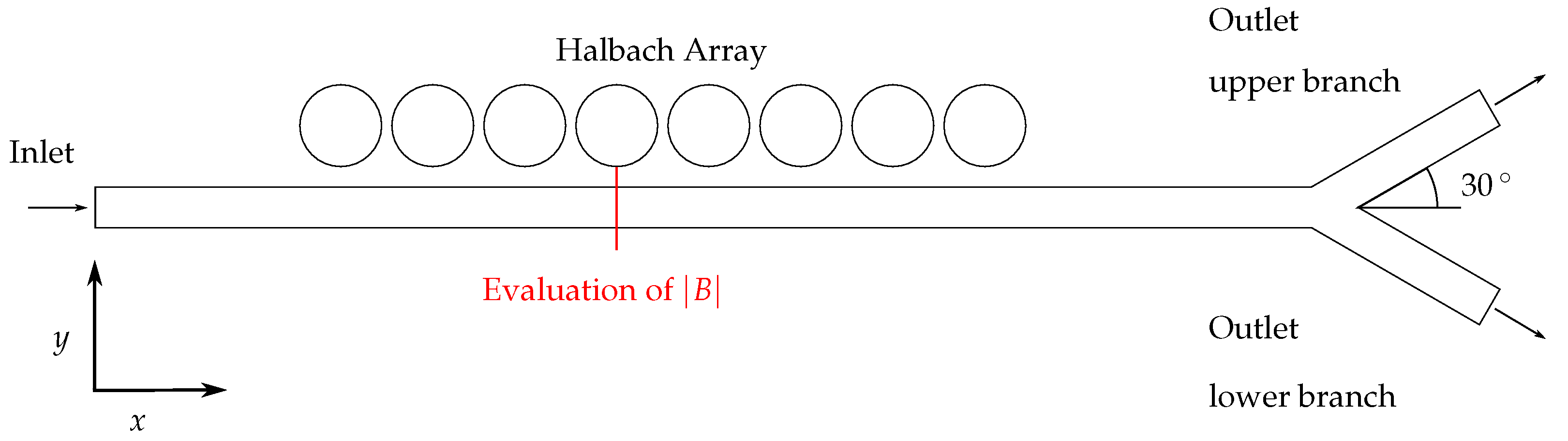
3.1. Model Definition

In this article, COMSOL Multiphysics® 6.1 is used to solve the magnetic field, fluid flow, and particle tracing equations in order to determine the steering performance in a 2D MDT scenario. To generate the magnetic flux density, a Halbach array consisting of rare-earth NdFeB PMs is utilized. The magnetic field is computed in a rectangular air-filled domain with a perfectly matched layer (PML) around it. The velocity flow consists of water and is assumed to be a Newtonian, incompressible, and single-phase laminar flow within a symmetrical Y-shaped bifurcation with an angle of 30 . One pulse of 100 SPIONs is released at the time t = 0 s. The SPIONs are uniformly distributed across the cross-section, corresponding to the distribution in real scenarios [90]. However, 2 mm each are left out at the top and bottom of the inlet since the background velocity is equal to zero at the vessel walls, and the SPIONs, therefore, also move very slowly close to the vessel walls. By doing so, the simulation time is shortened significantly. The simulation geometry is shown in Figure 5, and the fixed simulation parameters are summarized in Table 1. Moreover, the magnitude of the magnetic flux density | B | is investigated in detail at its strongest position for the strong side of the array. This position is highlighted in Figure 5.
To implement the model, three interfaces in COMSOL are necessary:
(1)
the “Magnetic Fields, No Currents (mfnc)” interface is used for generating the magnetic flux density;
(2)
the “Laminar Flow (spf)” interface is related to the velocity flow;
(3)
the “Particle Tracing for Fluid Flow (fpt)” interface is capable of mimicking particle trajectories in the velocity flow.
In this model, particle–particle and particle–fluid interactions are neglected. It is also assumed that attracted SPIONs do not influence the magnetic field distribution.

3.2. General Fluid Mechanics Model Considerations

To estimate the behavior of a velocity flow in tubes, channels, and vessels, two characteristic numbers are often calculated, namely the Reynolds number Re and the Péclet number Pe [72,91]. The dimensionless Reynolds number Re R + can be used to predict whether the flow profile is laminar or turbulent. It is defined by
Re = Inertial force Viscous force = u max R v η ,
where u max corresponds to the maximum velocity in the vessel (m/s), R v is the radius of the vessel (m), and η is the the kinematic viscosity of the fluid’s medium (m2/s) [91,92]. For pure water, η is equal to 10 6 m2/s [92]. For Re 2100 , the flow is assumed to be turbulent and for Re 2100 laminar, respectively [91]. With u max = 2 · u mean and the parameters in Table 1, we obtain Re = 100 2100 . This is in good accordance with the literature as for most blood vessels Re < 500 [91,93]. Therefore, in this paper, the velocity profile is expected to be fully laminar.
The movement of particles in a fluid is determined by both advective and diffusive flow. Which effect dominates can be estimated using the dimensionless Péclet number Pe R + [91,94] defined by
Pe = Advective transport Diffusive transport = 2 · u mean R v D .
Here, u mean is the average background velocity (m/s), R v is again the radius of the vessel (m), and D is the diffusion coefficient (m2/s). In the case of
Pe L v 2 R v ,
advective flow dominates [95]. According to [92], D of SPIONs is less than 10 11 m2/s. With Equation (17), Pe is less than 10 7 , which is much greater than L v / ( 2 R v ) = 30 . Therefore, advective transport is dominant for the chosen parameter setup of this paper.

3.3. Evaluation Procedure

In this study, the magnetic flux density with the resulting SPION distribution for a typical MDT scenario for different Halbach array scenarios is studied in order to evaluate the impact factors on the particle steering and find an optimized setup. By doing so, different parameters and scenarios were evaluated, which are described in detail in the following.

3.3.1. Evaluation of the Magnetic Flux Density and Its Gradient

At first, the distribution of the magnetic flux density B for the different magnetization angles ϑ { 30 , 45 , 60 , 65 , 75 , , 115 , 120 , 135 } between the single magnets is investigated in detail. The pattern of the arrays always starts with a magnetization direction in the negative y-direction. The number of magnets was set to N = 8 , and the distance between the array and the vessel was chosen as 0.5 cm. In addition, two simulations with ϑ = 180 were conducted. Here, the magnetization direction was in the ± y -direction and ± x -direction, respectively. The magnetization pattern for these simulations is illustrated in Figure 4.
In the next step, the array’s strong and its weak side are compared by evaluating the absolute value of the magnetic flux density in the vertical direction of the array at its strongest position. For an odd number of magnets, this is always underneath the middle magnet, and, for an even number, under the middle two magnets. In this paper, the magnitude of B was evaluated for N = 8 magnets in more detail. Thus, | B | was extracted underneath the fourth magnet, as highlighted in Figure 5.
Moreover, the extracted B underneath the fourth magnet is fitted for every magnetization angle ϑ for the strong and weak side to the exponential function depicted in Equation (15). By doing so, the absolute and relative fitting errors, as well as the fitting parameters k 1 and k 2 , are evaluated. From the fitting results, the gradient grad(B) is calculated for the strong and the weak side for every ϑ as the grad(B) is essential for the particle steering as the magnetic force is directly proportional to it (compare Equation (8)).

3.3.2. Evaluation of the SPION Distribution

From the perspective of magnetic drug targeting, the aim is to make the magnetophoretic force acting on particles stronger. As a result, the magnet attracts more particles to the desired region. Thus, for optimizing the Halbach array structure for a typical MDT scenario, the most important performance factor is the SPION distribution to the upper and lower branches, as well as the number of particles trapped by the magnets. In general, the stronger the force, the more particles take the upper branch or are trapped by the magnets and the less particles take the lower branch. Therefore, in this study, the SPION distribution on the upper and lower branches, as well as the ones trapped by the magnets for the geometry depicted in Figure 5, were investigated for different parameters of the linear Halbach array. The studied parameters are summarized in Table 2.
As the simulation time of the particle study is quite long, and much computational effort is necessary, we want to check if another magnetic parameter can be conducted in order to predict the particle distribution. Thus, next to the SPION distribution, additionally, the maximum gradient in the vessel grad(B)max and the total applied magnetic energy inside the vessel are derived for each investigated scenario. For the investigated 2D scenario in Figure 5, the total applied magnetic energy W m (J/m) is provided by
W m = 1 2 B , H d A vessel = ^ 1 2 B 2 μ 0 d A vessel ,
while integrating over the whole area cross-section of the vessel. Since the relative permeability of tissue and blood is approximately 1 [65], only the permeability of vacuum μ 0 is taken into account for the medium of the background flow.

3.3.3. Evaluation of the Magnetic and Hydrodynamic Drag Force

As the movement of SPIONs through the vessel mainly depends on the forces acting on the SPIONs, the two strongest forces F m and F d are investigated in this paper. These forces are evaluated using the extracted magnetic flux density as depicted in Figure 5 for N = 8 magnets and the vessel at a distance to the magnets of 0.5 cm. The magnetization angle ϑ was again varied in the range of ϑ { 30 , 45 , 60 , 65 , 75 , , 115 , 120 , 135 } . Aside from the forces, the ratio
F d - m = | F d | | F m |
is analyzed inside the vessel. The evaluation of the forces F m and F d is described in the following:
(1)
Evaluation of the (hydrodynamic) drag force F d :
The drag force is calculated in the main branch using Equation (7). Thus, it can be assumed that the drag force only has a component in the x-direction. As the velocity u = u x ( y ) · e x is assumed to be laminar and constant in the main branch, it has a parabolic profile, which is provided by
u x ( y ) = u max 1 y R v 2 ,
with u max = 2 u mean . y corresponds to the y-coordinate, and R v to the radius of the vessel.
(2)
Evaluation of the magnetic force F m :
The magnetic force pulls the particles towards the magnet. Thus, in this paper, F m is assumed to have only a component in the y-direction as a consequence of the fitted exponential decay of | B | in y-direction. This force is calculated according to Equation (14). Therefore, the particle’s magnetization M has to be known. It is determined by once reading out F m , y and the gradient grad(B) at a fixed location in the COMSOL simulation. Then, M is derived using Equation (14). For reasons of simplification, M is assumed to be constant. In the next step, F m is calculated using the fitted magnetic gradient for all ϑ .

4. Results

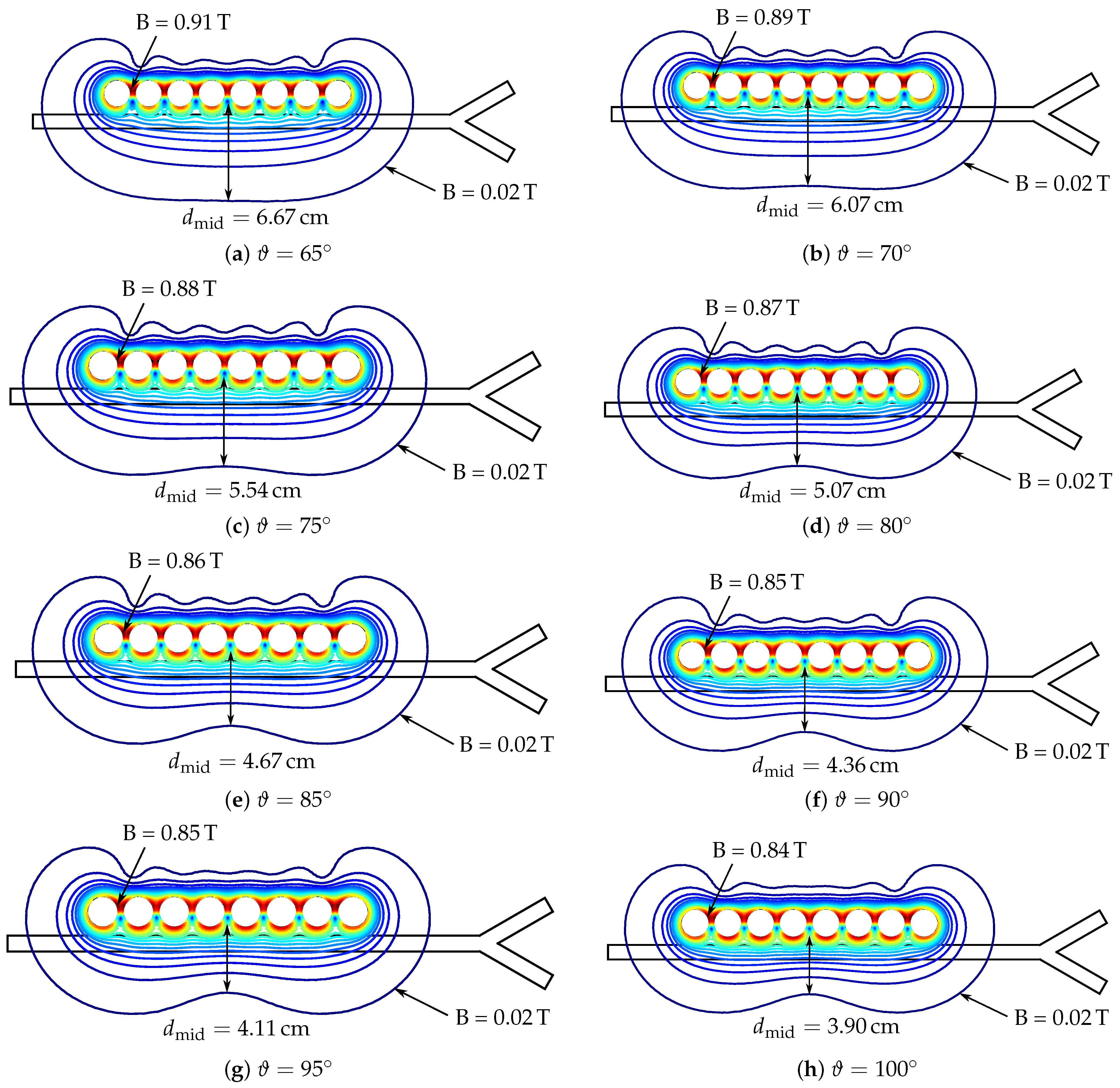
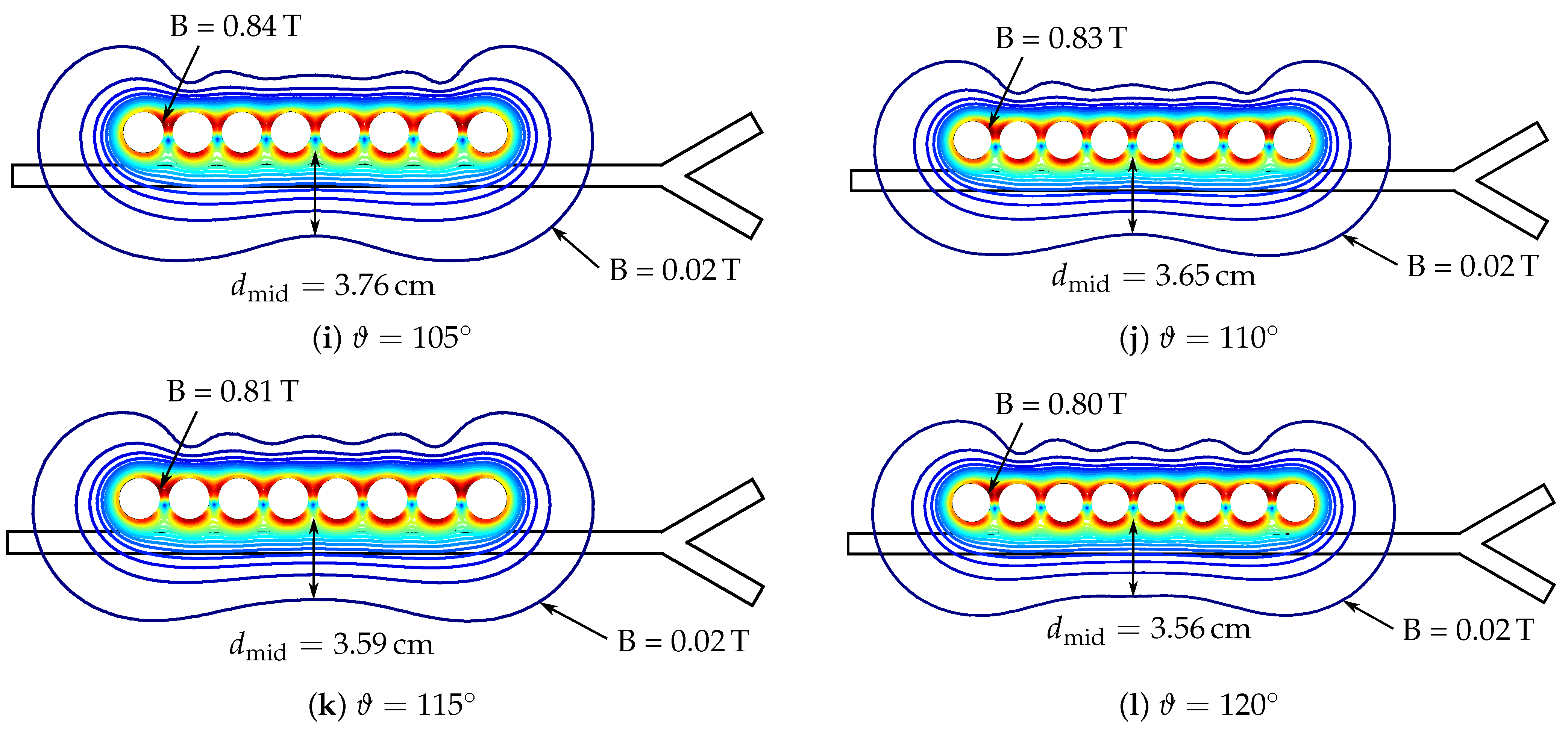
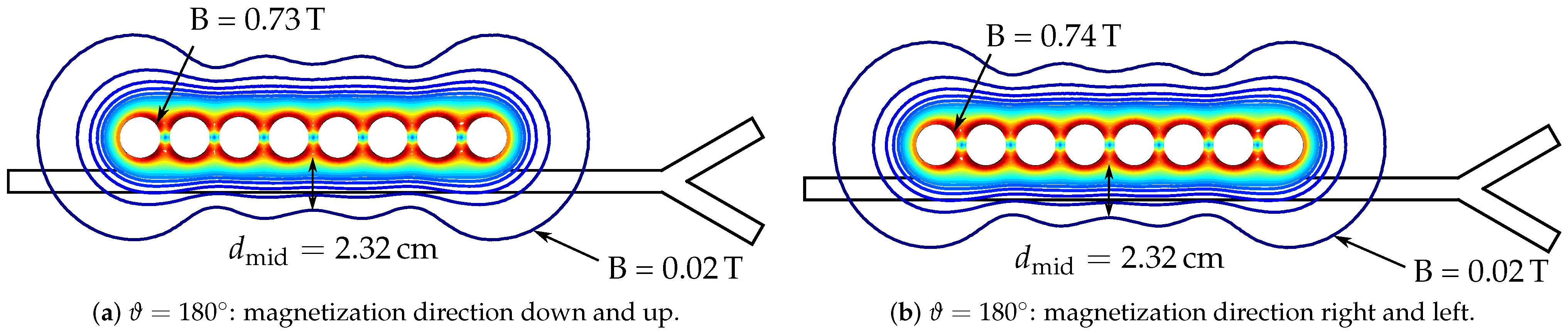
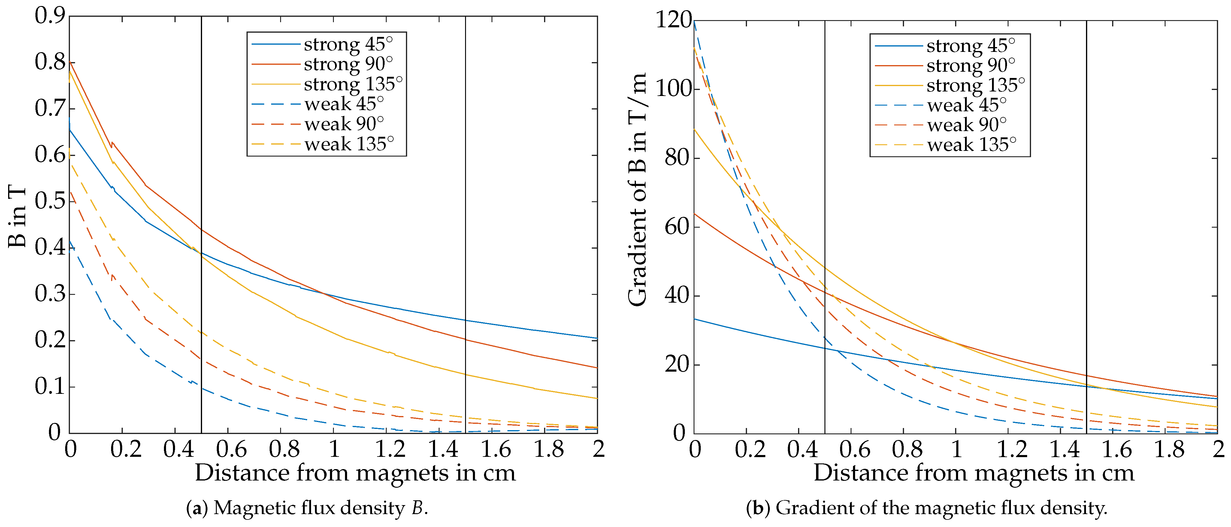
4.1. Evaluation of the Magnetic Flux Density

In Figure 6, the isolines of the magnetic flux density for varying magnetization angles ϑ between the single magnets are depicted. For comparison, the color map is the same for all subfigures. It becomes immediately observable that the Halbach array independent of the applied ϑ has a strong and a weak side. In the case of Figure 6, the strong side is facing the vessel. Furthermore, the field distribution of B is symmetric for all ϑ . This also holds true for an odd number of magnets. The maximum of the magnetic flux density B is always located between the first two and between the last two magnets, respectively. It can also be seen that B max decreases with increasing angle ϑ . Moreover, by comparing the shape of the isolines in Figure 6, it is visible that the magnetic field distribution is more compact for higher ϑ . This can be seen particularly clearly in Table 3. It shows that, for ϑ = 30 , the distance between the array and the outer isoline B = 0.02 T is still 10.91 cm. With increasing ϑ , the maximum distance d max decreases to d max = 3.87 cm for ϑ = 135 and is no longer in the center of the array. Moreover, the centered distance d mid decreases too. As a result, the field is much more homogeneous in the x-direction for higher ϑ . Figure 7 shows the magnetic flux density for ϑ = 180 with the magnetization direction in the ± x -direction and ± y -direction. It reveals that the shape of the magnetic flux density for the two simulations looks quite similar. Here, the field is even more compact with d mid = 2.32 cm, and the array no longer has a strong and a weak side.
The aforementioned compactness of the magnetic field distribution also influences the range of the magnetic flux density. This can be seen for chosen magnetization angles ϑ in Figure 8 on the left side. Overall, the flux density B is strongest for both the strong and the weak side of the array facing the vessel for large ϑ at the surface of the magnets but decays faster.

4.2. Evaluation of the Magnetic Gradient

In COMSOL Multiphysics® 6.1, the magnetic flux density is calculated numerically on a discrete mesh. This can be seen clearly in Figure 8 on the left side from the hard edges in the function of the strong side. Thus, it is hardly possible to derive the gradient of the magnetic flux density directly because many irregularities and noise would be present. Therefore, in this paper, the gradient is determined by first fitting B to the exponential function in Equation (15) and analytically deriving the fitted function:
B = ^ y B = k 1 k 2 e k 2 y
Figure 8 on the right side depicts exemplary results for the determined gradient. To see the trends, a small ( 45 ), middle ( 90 ), and big ( 135 ) magnetization angle are depicted and analyzed in more detail in the following.
Overall, the gradient in Figure 8 shows a clear difference between the weak and strong sides of the array. The gradient is stronger for the weak side of the array directly at the surface of the magnets but decays very fast with distance. For the strong side, it is vice versa. Thus, at a distance of approximately 0.5 cm, the gradient of the strong side is higher than the one of the weak side. When comparing grad(B) for the different ϑ in Figure 8, it is noticeable that, for both the strong and the weak sides, the gradient is larger for higher angles. For the strong side, the curves converge again at a distance of about 1.5 cm from the magnets’ surface, while the curves of the weak side still do not intersect at a distance of 2 cm.

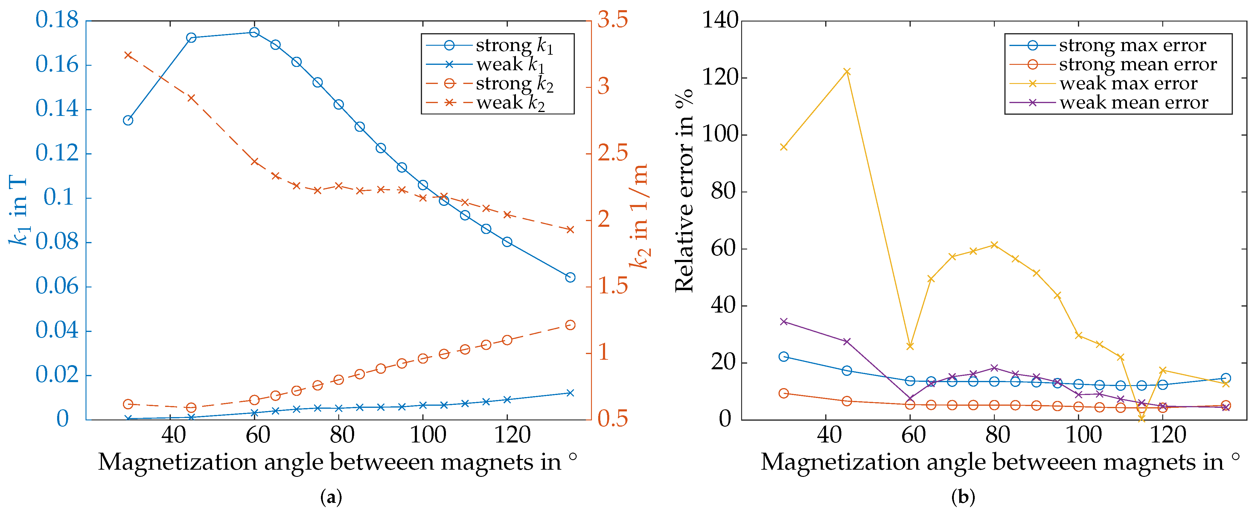
4.3. Evaluation of the Fitting of the Magnetic Flux Density

As mentioned in the previous section, the gradient of the magnetic flux density was determined by fitting the magnetic flux density to the exponential approach in Equation (15). The mean and the maximum fitting error ε mean and ε max for all ϑ as absolute and relative errors are summarized in Table 4 for the whole evaluation domain as well as only limited to a distance inside the vessel. Furthermore, the fitting parameters k 1 plus k 2 and the relative fitting error are depicted in Figure 9.
Overall, the fitting performance for the strong side performs well with ε mean = 5.3 % and ε max = 13.1 % over the whole evaluation domain. Moreover, as the right plot in Figure 9 shows, the error is relatively constant for the strong side over the magnetization angle ϑ . However, the fitting results for the weak side are, with an error of ε mean = 13.6 . 3 % and ε max = 45.8 %, inadequate. Especially for the small angles ϑ = 30 and ϑ = 45 as well as for angles in the range ϑ 65 , 95 , the relative fitting errors are insufficiently high.
Next to the relative fitting error, the left plot in Figure 9 also shows the values for fitting parameters k 1 and k 2 . Overall, the amplitude parameter k 1 is approximately a factor of 100 higher for the strong side compared to the weak side. For the strong side, k 1 has its maximum at ϑ = 60 with k 1 = 17.5 mT and decays with increasing ϑ . On the other hand, for the weak side, k 1 increases with increasing ϑ . The exponent parameter k 2 , in contrast, is greater for the weak side of the array. Here, k 2 increases with increasing ϑ for the strong side and decreases with increasing ϑ for the weak side of the array, respectively.

4.4. Evaluation of the Parameter Study on the SPION Distribution

The main evaluation parameter in particle steering is the distribution of the SPIONs to the upper and lower branches as well as the percentage of the particles trapped by the magnets. This section presents the results for the different influence parameters on the SPION distribution in detail, namely the influence of the weak vs. strong side of the array, the quantity of magnets (Figure 10), the magnetization angle ϑ between the single magnets (Figure 11), and the distance between the magnetic array and vessel (Figure 12). In addition, the results for the maximum gradient grad(B) and the total applied magnetic energy W m inside the whole vessel are opposed.

4.4.1. Influence of Weak vs. Strong Side of the Magnet Array

A Halbach array has a strong and a weak side, resulting out of the constructive and destructive overlapping of the magnetic fields of the single magnets. Thus, fewer particles should be trapped if the weak side is applied to the vessel. This can especially be seen in Figure 11 and Figure 12, where the number of trapped particles is much higher for the strong side (blue lines). The number of SPIONs taking the lower branch is lower for the strong side.

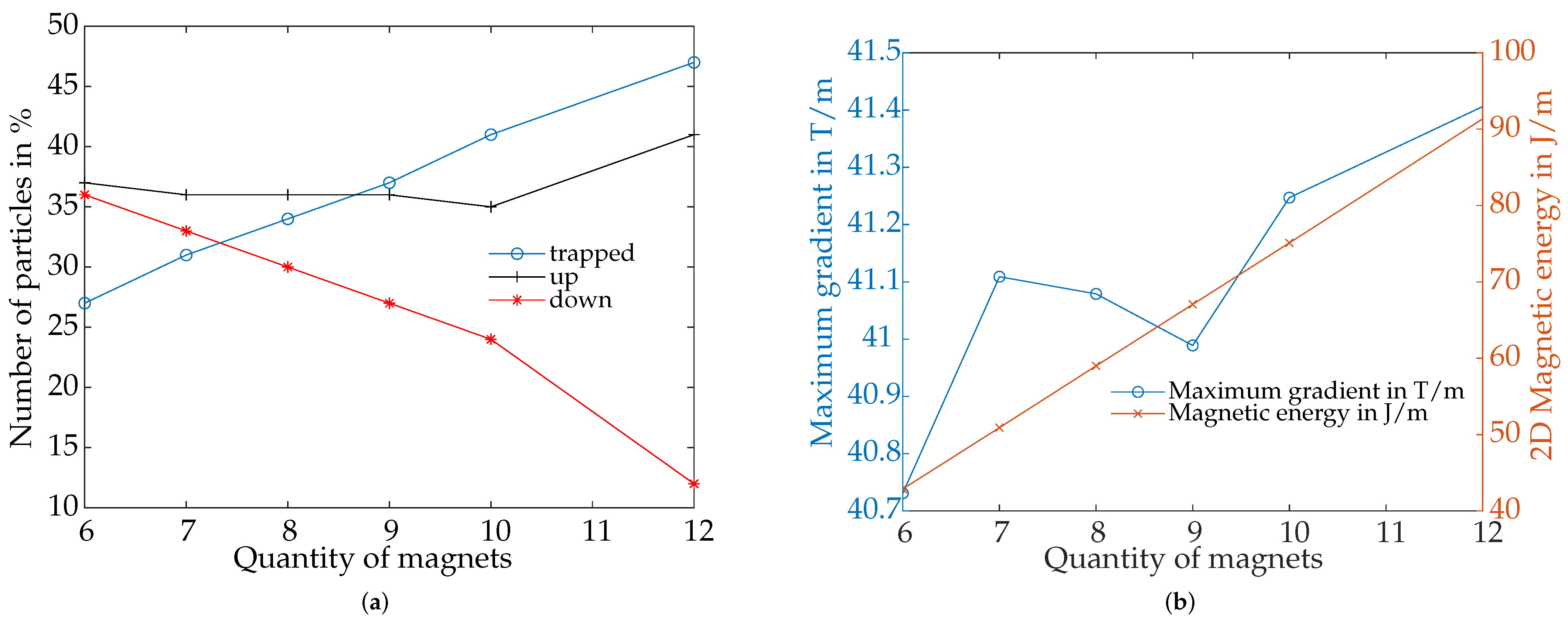
4.4.2. Influence by Quantity of Magnets

A Halbach array consisting of more magnets means a longer array, and, therefore, the time when a magnetic force is applied to the particles while propagating underneath the array is longer. This can be seen in Figure 10a on the left side, where the SPION distribution for the strong side of the array over the number of magnets is depicted. The more magnets are used, the more SPIONs become trapped, and the less SPIONs take the lower branch.
In Figure 10b, the corresponding maximum gradient in the vessel and the magnetic energy calculated according to Equation (19) are plotted. The maximum gradient is always located below the middle magnet (odd number of magnets) or the middle two magnets (even number of magnets). The influence on the maximum gradient in the vessel is negligibly low (see axis scale in Figure 10). On the other hand, the magnetic energy in the vessel increases linearly with longer magnetic arrays.

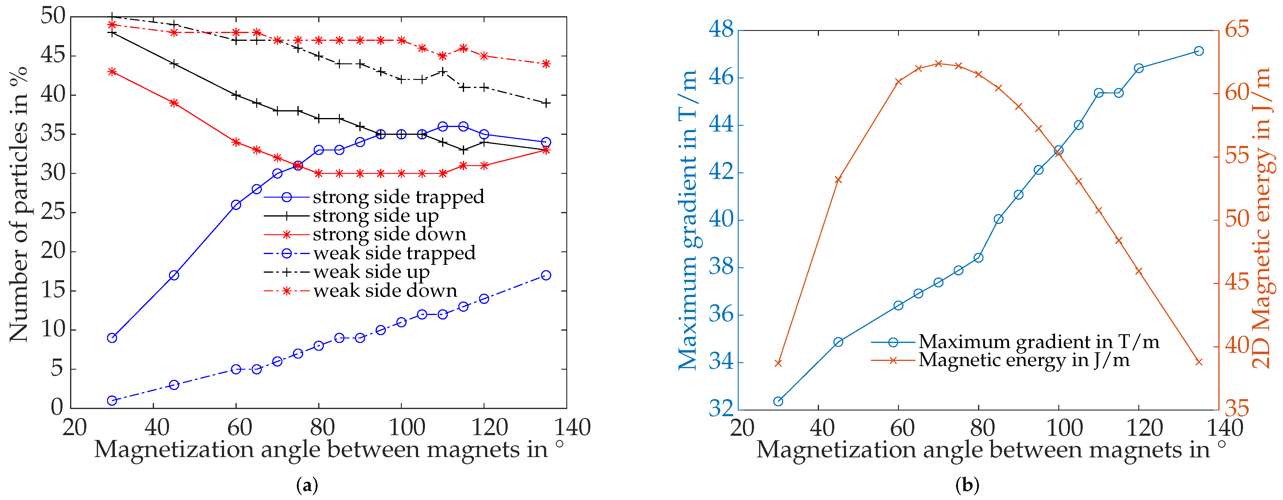
4.4.3. Influence of Magnetization Angle between Magnets

To the best of the authors’ knowledge, in the literature, the influence of the magnetization angle ϑ has not been investigated for MDT so far. However, Figure 11a reveals that the magnetization angle ϑ between the magnets also plays an important role in influencing the particle movement. Overall, a higher magnetic force corresponds to a higher number of trapped particles and a smaller number of SPIONs taking the lower branch. In Figure 11, it can be seen that, for the strong side of the array, higher angles cause more trapped particles till a magnetization angle of 120 . The maximum number of trapped particles is approximately 1/3 of all particles (36 of 100). Interestingly, higher angles than 120 reduce the number of trapped particles again. The minimum number of SPIONs taking the lower branch is 30% for ϑ 80 , 110 . For the weak side of the array, with increasing ϑ , the number of trapped SPIONs increases approximately linearly, and the number of SPIONs taking the lower branch decreases approximately linearly, respectively.
Figure 11b shows the trend of the maximum gradient and the magnetic energy in the vessel. The maximum gradient starts at 32.4 T/m at 30 and increases nearly linearly with the magnetization angle to 47.1 T/m at 120 . The magnetic energy in the vessel is low for small and high ϑ . It has its maximum between ϑ = 60 and ϑ = 90 .
The results for higher magnetization angles are listed in Table 5. It compares the particle distribution plus the maximum gradient, and magnetic energy for the two simulations with a magnetization angle ϑ = 180 . The results reveal no influence in the SPION distribution either in the maximum gradient or magnetic energy in the vessel for arranging the magnetization direction in the ± x -direction or ± y -direction.

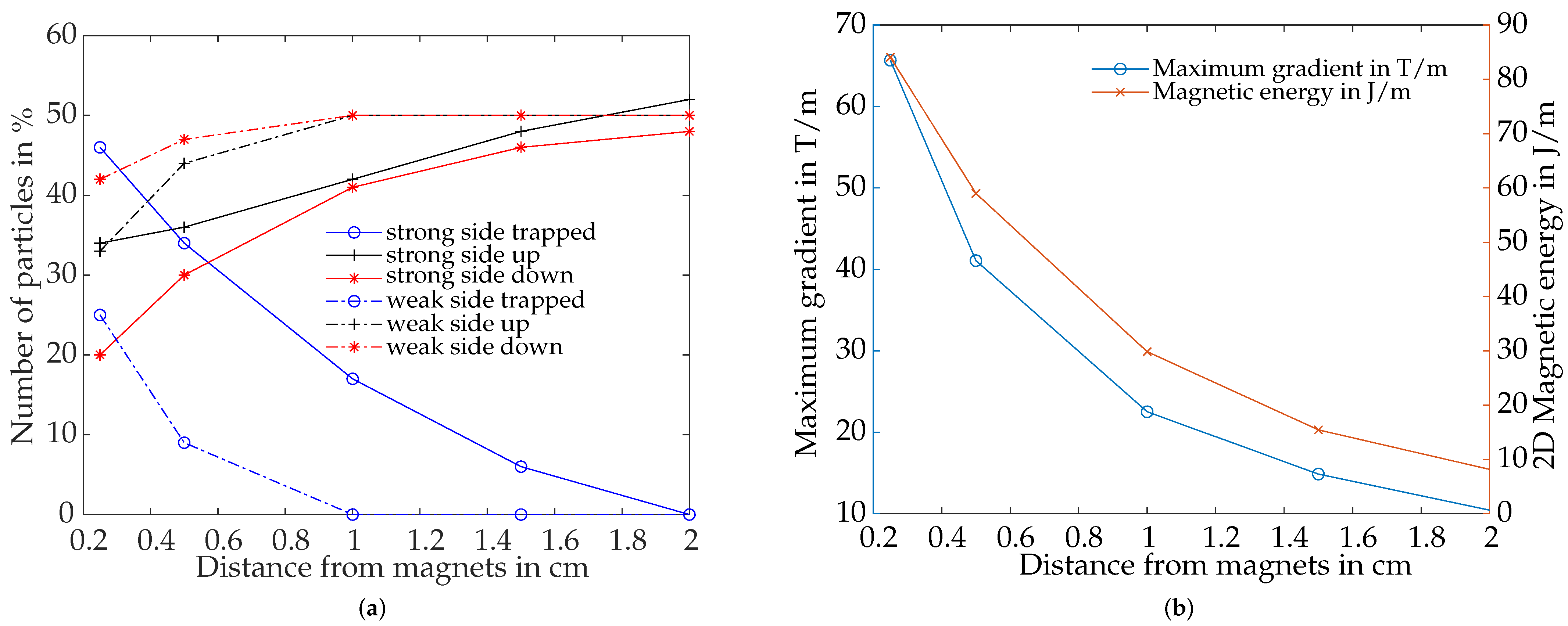
4.4.4. Influence of Distance between Magnetic Array and Vessel

Figure 12 reveals that varying the distance between the array and the vessel also influences the simulation results. Overall, a higher distance between magnets and vessel corresponds to a weaker magnetic force on the SPIONs. Thus, with increasing distance, the number of trapped SPIONs reduces for both the strong and the weak side of the array. For the strong side, the number of SPIONs taking the desired upper branch increases approximately linearly with the distance and obtains 52% at a distance of 2 cm even over the 50% distribution without an applied magnet. For the weak side of the array and at a distance of 1 cm, the SPIONs spread equally to the upper and lower branch, and no particle is trapped by the magnets anymore. Thus, at a distance of 1 cm and greater, the magnetic force does not influence the chosen parameter setup. Figure 12b shows that, with increasing distance, both the maximum gradient and the magnetic energy in the vessel decrease.

4.5. Evaluation of the Magnetic and Hydrodynamic Drag Force

As the movement of the SPIONs can be predicted when knowing the forces acting on the SPIONs, in this section, the two main forces, namely the magnetic and (hydrodynamic) drag force ( F m and F d ), are investigated in more detail. Both forces are calculated for the strong and weak sides of the array underneath the fourth magnet, as illustrated in Figure 5. The resulting magnitudes of the forces are depicted in Figure 13.

4.5.1. Evaluation of F d

As aforementioned, the drag force is calculated based on Equations (7) and (21). Thus, due to the parabolic velocity profile, F d has its maximum at the center line of the vessel with | F d , max | 9.4 · 10 11 N, and a minimum magnitude of 0 N at the vessel wall. This can also be seen in Figure 13. Furthermore, as the drag force is the force washing the particles within the background velocity, it only has a component in the x-direction.

4.5.2. Evaluation of
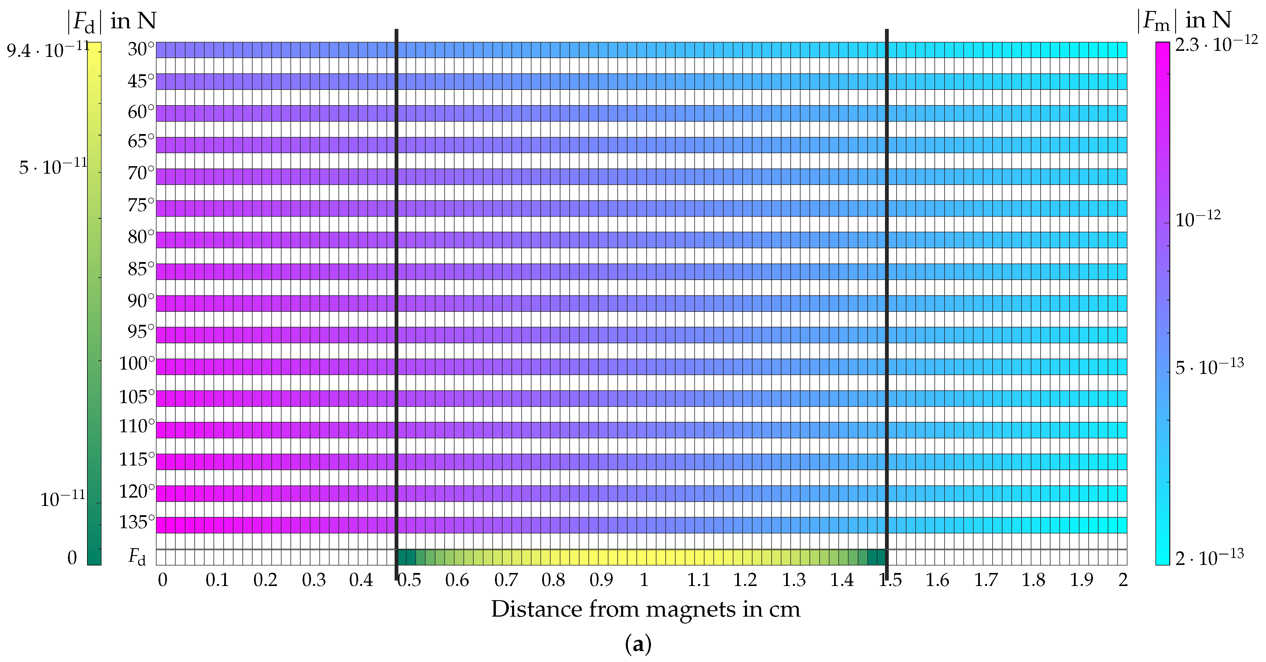
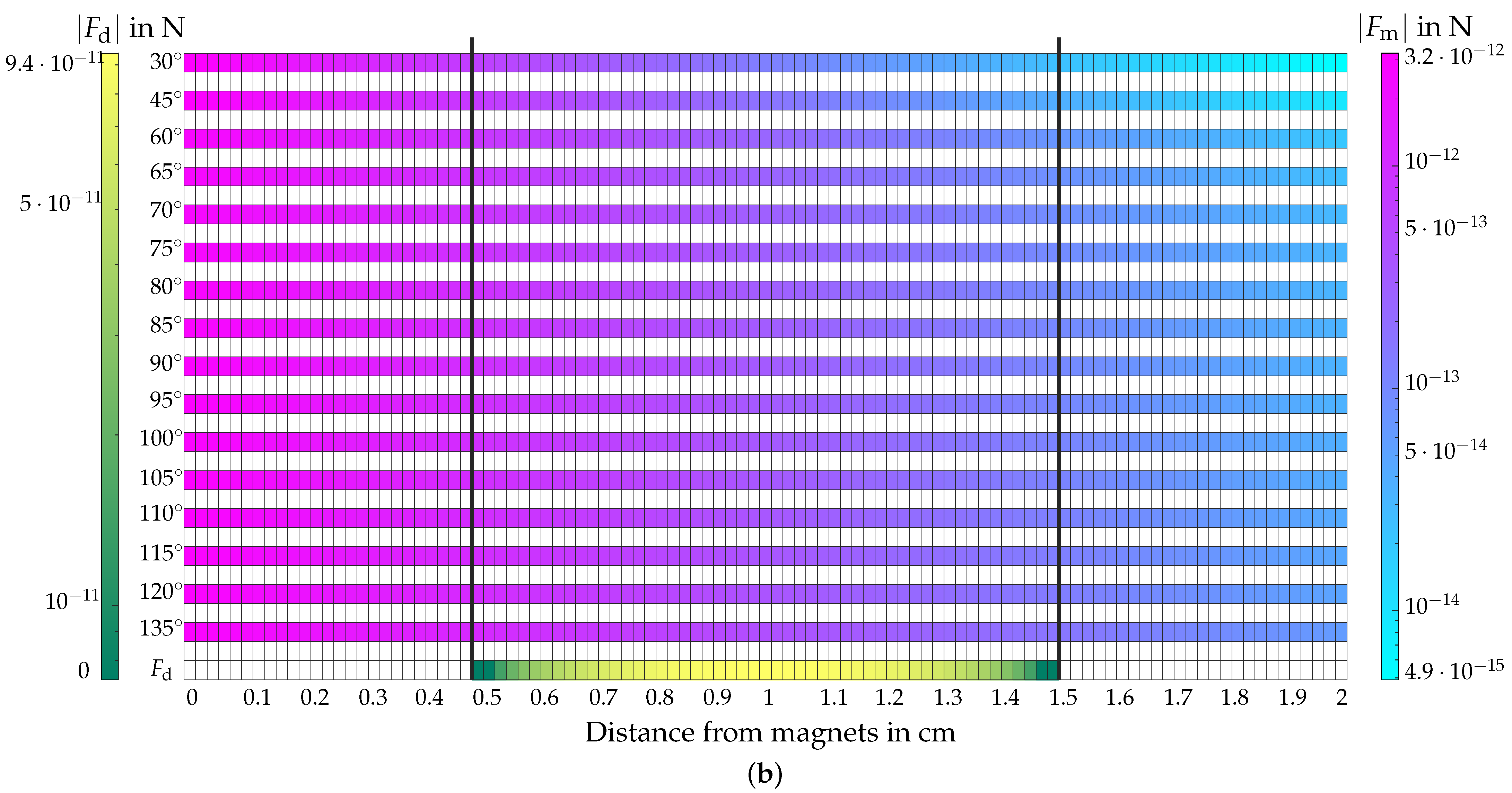
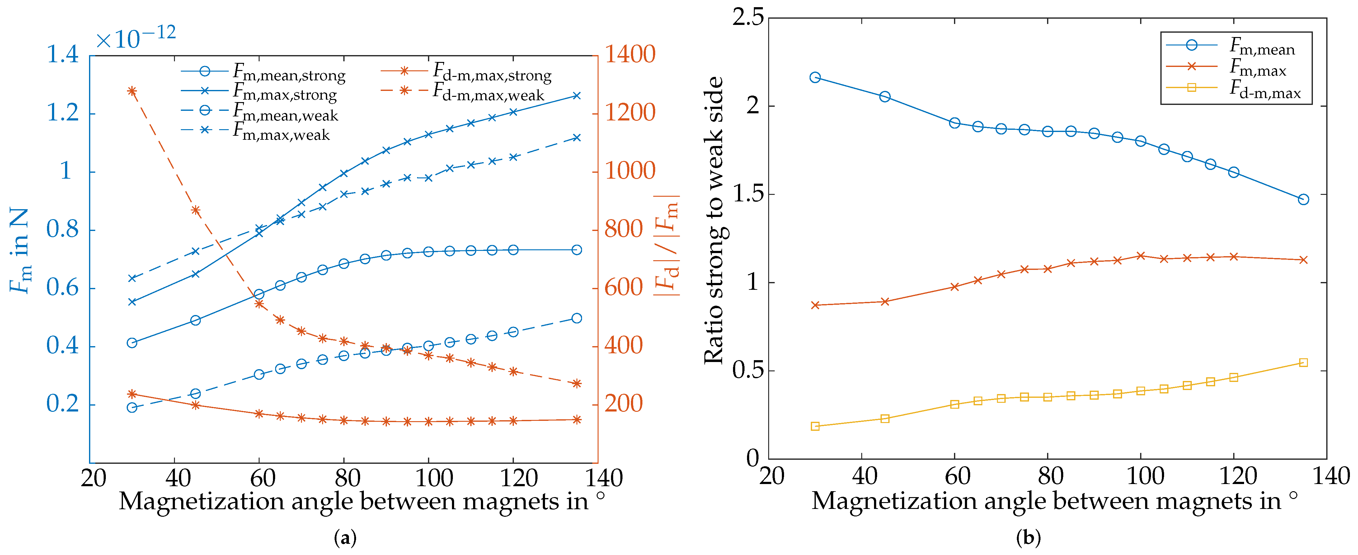
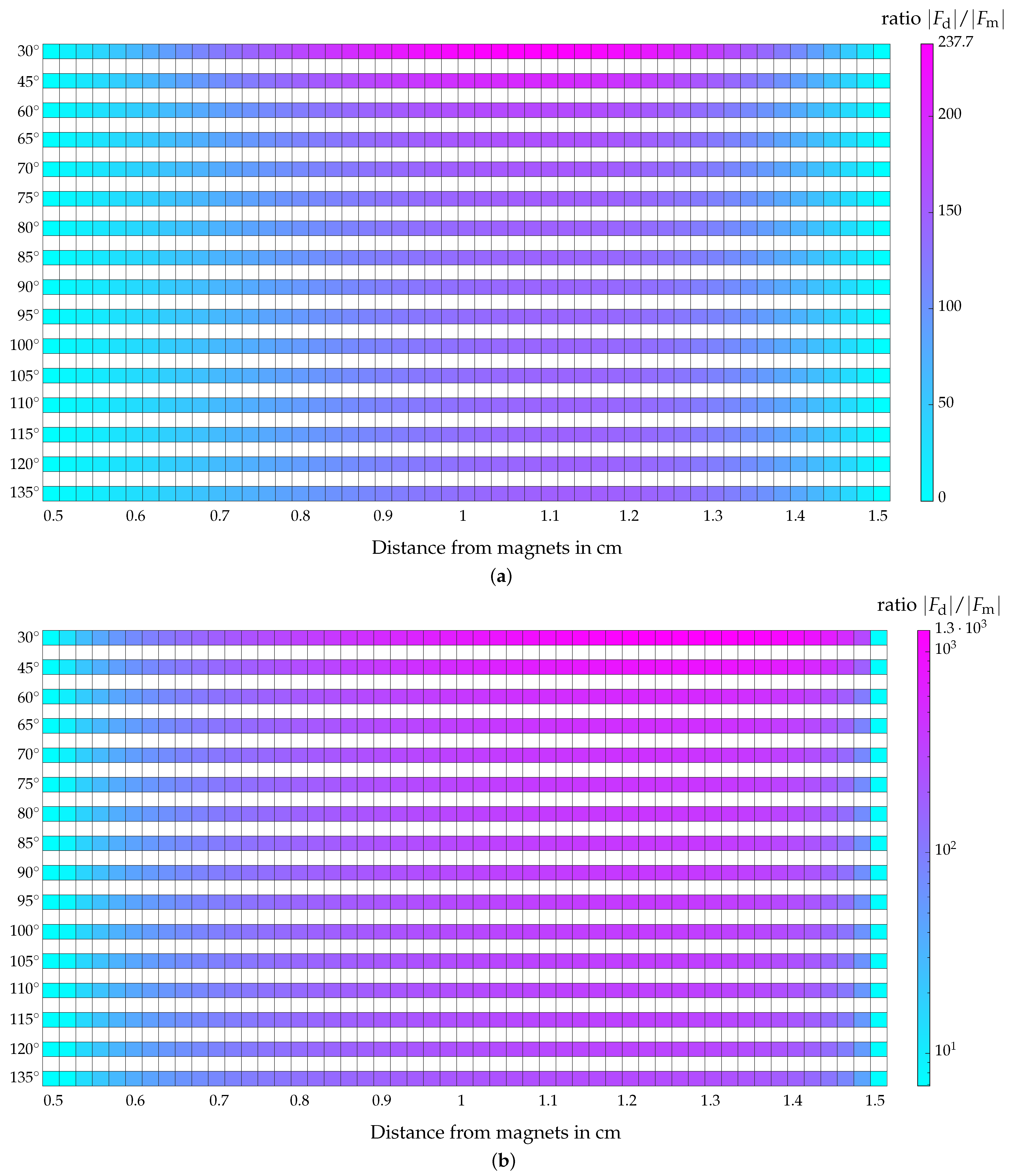
 F m

On the contrary, the magnetic force F m pulls the SPIONs towards the magnet. Thus, it mainly has a component in the y-direction. Before the magnitude of the magnetic force can be calculated according to Equation (14), the magnetization M of one SPION has to be determined. For this purpose, F m , y = 8.38 · 10 13 N and grad ( B ) = 32 T/m are extracted from a fixed position in the simulation. Then, M 4 · 10 5 A/m is derived using Equation (14). This value is in good accordance with the magnetization values of SPIONs with regard to [5,96,97]. By applying M = 4 · 10 5 A/m to Equation (14), the magnetic force reaches values from 2 · 10 13 N to 2.3 · 10 12 N inside the vessel for all magnetization angles ϑ for the strong side of the array (compare Figure 13). For the weak side of the array, the magnetic force was in the range of 4.9 · 10 15 N to 3.2 · 10 12 N for all ϑ .
Figure 13 shows that the magnitude of F m decreases with the distance to the magnets. Thus, for both sides of the array, the strongest force is at the vessel wall closer to the magnets and the weakest at the vessel wall further away from the magnets, respectively. For the strong side, F m is much higher for greater ϑ , whereas, for the weak side, the influence of ϑ is much smaller. This can also be seen in Figure 14a, where the mean and maximum values of F m for the weak and the strong side for all ϑ are depicted. In Figure 14b, the ratio between the strong and the weak side is shown. By comparing the magnitude of F m for the strong and the weak sides, it reveals that F m is for all ϑ approximately double (factor of ≈1.85 for ϑ [ 60 , 100 ] ) as high for the weak side compared to the strong side. For ϑ = 135 , the difference is only a factor of approximately 1.5. However, as Figure 13 shows, the magnetic force decays much faster for the weak side, and at a distance of 2 cm to the magnets, | F m | is approximately a factor of 100 stronger for the strong side. In addition, Figure 14 reveals that the maximum magnetic force inside the vessel for the weak side is for small ϑ higher than for the strong side. However, this difference becomes smaller with increasing ϑ , and, for ϑ > 65 , F m , max is greater for the strong side again. Nevertheless, as shown on the right plot in Figure 14, the ratio between strong and weak side for the maximum value of the magnetic force is relatively small for all ϑ .

4.5.3. Comparison of F m and F d

Since the ratio of magnetic to drag force is particularly relevant for the direction of motion of the SPIONs, this ratio is illustrated in Figure 15. The ratio F d - m is equal to zero at the vessel walls as F d = 0 N there. The maximum values for the strong and the weak side of the array are located at a distance between 1 cm and 1.3 cm from the magnets.
Overall, the ratio for the weak side is much higher than for the strong side as the magnetic force is weaker for the weak side. This can also be seen in Figure 14, where the mean and maximum value of F d - m for both sides of the array are depicted on the left plot, and the ratio between these two sides on the right plot. Moreover, Figure 15 reveals the influence of the magnetization angle ϑ . Whereas the influence is negligible for the strong side, for the weak side and ϑ = 30 , F d - m , max is with 1279 very high and decreases with increasing ϑ . For ϑ = 135 , F d - m , max is only 274. The same trend can be seen in the ratio on the right plot in Figure 14 too. For ϑ = 30 , the ratio F d - m , max is only approximately 0.19 and increases to F d - m , max = 0.55 for ϑ = 135 .

5. Discussion and Limitations of This Study

This paper conducted a systematic parameter study with the focus on varying the magnetization angle for steering SPIONs in a typical MDT scenario using a linear Halbach array as a magnetic field source. In this section, the results are discussed in detail in order to build an optimized array for particle steering. In addition, the content is compared with the state-of-the-art approaches in MDT and the limitations of this work are identified.

5.1. Discussion of the Magnetic Flux Density and Its Effect on Particle Steering

In the ideal case, a Halbach array has a one-sided magnetic field caused by constructive and destructive inference on each side of the array [76,77,88]. However, as can be seen in Figure 6, this superposition effect is not ideal due to the air space between the magnets and their round shape. As shown in Section 4.1, the magnetic flux density is more compact for a higher magnetization angle ϑ (between ϑ = 30 and ϑ = 135 , there is approximately a factor of 2.8 for d max and 3.3 for d mid , respectively). Thus, this paper assumes that the magnetic flux density is constant in the x-direction. This assumption has already been proven and discussed in [43,51] for a Halbach array with a magnetization angle of ϑ = 90 , where the resulting standard deviation was approximately a factor of 50 smaller than the mean magnetic flux density. Sharma et al. [98] investigated the magnitude of the magnetic force in the x- and y-directions for one single permanent magnet. They also concluded that the force in the y-direction is dominant. On the other hand, Bernad et al. [99] showed that the difference in F m , x and F m , y depends on the shape of the magnet. However, the SPIONs accelerate before the magnet and decelerate after the magnet due to the magnetic force. When the magnetic field source is symmetric, this effect is approximately canceled out. Nevertheless, as can be seen in Figure 13, Figure 14 and Figure 15, the magnitude of the drag force | F d | is much higher, and, therefore, it can be assumed that the impact of the magnetic force in the x-direction can be neglected.
Figure 10 shows that the quantity of magnets in the array, and thus the length of the array, significantly influences the particle distribution. A Halbach array with a higher number of magnets means a larger area where the magnetic field can influence the particles in the vessel. Thus, the magnetic force has more time to act on the particles in the case of a more extended array. Also, the magnetic field itself becomes larger with more magnets. Consequently, more particles are attracted to the wall of the vessel where the array is placed. In our recently published letter [41], we showed that the sorting performance depends primarily on the total magnetic effort in terms of the applied magnetic energy. Here, it was shown that a more extended array with a lower magnetic field strength has the same impact on particle propagation as a shorter array with a higher field strength measured in terms of investigated magnetic energy. Figure 10b in this paper shows that the magnetic energy increases with increasing number of magnets too. On the other hand, the maximum gradient in the vessel is relatively constant because more magnets do not really influence the change in the magnetic field. Therefore, the magnetic field of the added magnets has a very low influence on the high magnetic field area between the magnets.
In [51], it was stated that, by decreasing the distance d m between the single magnets, the magnetic flux density becomes more homogeneous, and thus, the superposition effect becomes stronger. However, because of the torque, the distance between the magnets is crucial for mechanical stability [88]. In general, mechanical stability is an essential factor that must be considered for the practical implementation of the presented steering approach. For example, the two simulations with ϑ = 180 show equal results regarding the isolines of the magnetic flux density (compare Figure 7), and the SPION distribution, the maximum gradient, and the energy in the vessel were equal (see Table 5). However, of course, the setup with magnetization directions down and up is mechanically stable, whereas the magnets in the array with the magnetization directions right and left repel each other.
In addition to the strength of the magnetic force, its effective range is another crucial factor. In general, there is a trade-off between the strength of the magnetic force and its effective range. This becomes particularly obvious when comparing the strong and weak sides of the array: Figure 8b shows that the gradient of B (directly proportional to the magnetic force) for the weak side of the array is stronger close to the array than for the strong side but decays much faster. A similar effect can also be seen in Figure 13. Here again, the magnetic force close to the array is stronger for the weak side than for the strong side. We can, therefore, conclude that it would be desirable to have a constant gradient over the vessel’s diameter. If the gradient closer to the vessel wall increases, this expedites the trapping of particles. Obviously, the desired range depends strongly on the particular application. Thus, Ijiri et al. [52] separated different sizes of the magnetic nanoparticles in a tube close to the surface of a 47-magnet Halbach array, which was arranged so that the weak side faces the tube. However, especially in MDT, a high range of magnetic force is essential to steer the particles in deeper body regions. Therefore, in most cases, the strong side of the Halbach array is used in MDT [46,47,49,100]. The magnetization angle ϑ between the magnets influences the shape of the magnetic field. Figure 6 shows that the field underneath the vessel becomes compressed with higher magnetization angles. Therefore, the magnetic field lines in the vessel area are closer to each other, which means that the field is stronger and can influence the particles more strongly. Thus, more particles become attracted to the upper vessel wall. This also affects the effective range of the magnetic flux density and its gradient. For larger ϑ , the gradient of B (and thus the magnetic force) directly at the magnets is greater but then also decays more strongly. However, in our considered distance range, the gradient of B for large ϑ is always higher than that of smaller angles, so larger ϑ are preferable for determining a higher range. This is in good accordance with the results for the particle distribution in Figure 11 and with the mean and maximum magnitude of | F m | in Figure 14. Here, the mean value of the magnetic force was the strongest for ϑ [ 80 , 100 ] .
The same trend can be seen for the weak side of the array. As suggested in our previous work, the strong and weak sides can be switched by mechanical rotation of all single magnets [43,51] or by changing the current direction of EMs [46], to wash the trapped particles off. This requires the weakest possible force (and therefore the weakest possible gradient) on the weak side. Figure 8 shows that this is the case for small magnetization angles. Thus, switching between the strong and weak side results in a trade-off between a field with a long effective range (large ϑ ) on the strong side and a field with a short effective range (small ϑ ) for the weak side. By evaluating the ratio between the strong and the weak side, as shown in Figure 14b, the best trade-off is approximately in the range of ϑ [ 60 , 100 ] . Since, as aforementioned, the simple production of the array is also an important design criterion, ϑ = 90 seems to be a good choice. Furthermore, for easy switching between the strong and the weak side, the use of EMs as in [46] is recommended.

5.2. Discussion of the Fitting Results

As the magnetic force is directly proportional to the gradient of the magnetic flux density, it is worth investigating the gradient over the vessel cross-section in detail. For determining the gradient, the magnitude of B along the evaluation line (depicted in Figure 5) was fitted to the exponential approach in Equation (15) and afterwards derived analytically as shown in Equation (22) for the strong and the weak side of the array and various magnetization angles ϑ . As Figure 9 and Table 4 depict, the fitting results for the strong side were quite good (mean fitting error of ε mean = 5.3 %) but insufficient for the weak side, with a mean error of ε mean = 13.6 % and individual maximum errors of up to ε max = 122.3 %. Especially for the weak side and small ϑ , the fitting results were poor. The reason for this can be found in the shape of B for these cases. For example, Figure 8a shows that B of the weak side for ϑ = 45 at a distance of approximately 1.8 cm rises slightly again. This, of course, contradicts the assumed strictly monotonic decrease in the exponential fitting function. Since the field strength values are also very small ( ε mean = 4.2 mT), this results in significant relative errors. Nevertheless, as the magnitude of the magnetic field strength and the magnetic gradient are small, the magnitude of the magnetic force is small as well. Thus, the drag force dominates the magnetic force anyway. For this reason, despite the high relative errors, the calculations in this paper continue with the fitted values for the consideration of the forces. For a more accurate fitting result, as in [51], fitting functions with more degrees of freedom or analytical approaches, such as in [56,57,101], must be used.

5.2.1. Discussion of Fitting Parameter k 1

Fitting parameter k 1 corresponds to the magnetic flux density’s amplitude factor. As shown in Figure 9, k 1 is approximately a factor of 100 stronger for the strong side than for the weak side. By inserting the fitted magnetic flux density of Equation (22) in Equation (14), the magnetic force can be expressed as
F m , y = V p M | B | = V p M k 1 k 2 e k 2 y .
It is obtained that the magnitude of the magnetic force is directly proportional to the factor k 1 . Therefore, the greater k 1 , the greater the magnitude of the magnetic force | F m | . However, as Equation (23) depicts, the exponential parameter k 2 also contributes to | F m | . For this reason, the results that a greater k 1 corresponds to a greater | F m | cannot be seen in Figure 13, Figure 14 and Figure 15.

5.2.2. Discussion of Fitting Parameter k 2

As aforementioned, k 2 corresponds to the exponential fitting parameter. As Figure 9 shows, k 2 is much greater for the weak side of the array than for the strong side. By determining the gradient of B, this parameter is both in the exponent and directly proportional to the amplitude of the magnetic force | F m | (compare Equation (23)). This means that k 2 influences both the range of the effective magnetic force and its magnitude. For a large magnitude of | F m | , k 2 should be large, whereas, for an extensive range, k 2 should be small. This results in a trade-off, which depends on the requested application. As a more extensive range is required for MDT, k 2 should tend to have lower values here. This can also be seen in the simulation results. For the strong side of the array, the maximum force | F m | is much lower due to the small k 2 (Figure 9 and Figure 13), but the effective range in the y-direction is much greater in this case so that more SPIONs are deflected (Figure 11).

5.3. Discussion of the Maximum Gradient and Magnetic Energy for Predicting Particle Steering

Since the analysis of the particle distribution is very complex, this section will examine whether the evaluation of the maximum gradient in the vessel or the total applied 2D magnetic energy in the vessel can also be used to determine the particle distribution. The variation in the quantity of magnets in Figure 10 shows that the magnetic energy increases linearly with the quantity of magnets. A Halbach array with a higher number of magnets means a longer time when the magnetic field can influence the particles in the vessel. Also, the magnetic field itself becomes greater with more magnets. Consequently, more particles will be attracted to the wall of the vessel where the array is placed. This trend can be seen for the trapped SPIONs in Figure 10 and follows the same trend as the magnetic energy in the vessel. On the other hand, the maximum gradient in the vessel is relatively constant because more magnets do not influence the magnetic field change in y-direction that much. The highest gradient is between the single magnets. The magnetic field of the added magnets has a very low influence on the high magnetic field area between the magnets. The change in the total magnetic energy in the vessel is much more significant in this case because a higher number of magnets means a larger area with an applied magnetic field. Summarized, these results show that the maximum gradient is unsuitable for predicting the particle distribution. In contrast, Figure 12 shows the particle distribution over the distance between the vessel and the magnetic array. Here, it can be observed that the trend of the magnetic energy and the maximum gradient corresponds well with that of the trapped particles.
The magnetization angle ϑ between the magnets influences the shape of the magnetic field (see Figure 6). As Table 3 shows, with higher angles, the field underneath the vessel becomes compressed. Therefore, the magnetic field lines in the vessel area are closer, which means that the field is stronger and can influence the SPIONs more, resulting in more trapped particles. The corresponding SPION distribution is depicted in Figure 11. For ϑ [ 80 , 110 ] , the fewest particles take the lower output. This means the magnetic force is strongest here, and the effective range is highest. On the other hand, most SPIONs are trapped for ϑ > 95 . This means that the magnetic force is strongest near the magnets. These effects can also be recognized in Figure 13. Nevertheless, the magnetic energy is highest in the range of 60–80 ° and decreases for higher angles. The maximum gradient, on the other hand, increases approximately linearly. However, neither trend matches the SPION distribution.
Overall, the trends of the maximum gradient in the vessel and the magnetic energy in the vessel deviate from the results of the SPION distribution. Therefore, neither parameter is suitable for predicting the particle distribution. Thus, it is better to consider the total magnetic force. In this paper, the magnetic force was only analyzed at its strongest position. However, we showed in our previous publication [51] that the magnitude of the magnetic force depends strongly on the evaluated position, especially for the strong side of the array. Therefore, we recommend evaluating the particle distribution, although the simulation effort is much higher.

5.4. Comparison with the State-of-the-Art Research

In the following, the investigations of this paper are compared with the state-of-the-art research for steering magnetic nanoparticles in an MDT scenario. An overview of the corresponding studies with their field sources, evaluation parameters, and a summary of the studies’ aims is provided in Table 6. The steering results are not included in Table 6 as the performance depends significantly on the analyzed geometry, the overall setup, and parameters such as the investigated particle size. As these parameters differ considerably in the analyzed publications, comparing the steering performance is not meaningful.
As the simulation time of the particle study is quite long, and much computational effort is necessary, many researchers evaluated other magnetic parameters in order to predict the particle distribution. In Table 6, an overview of the evaluated parameters is provided. Here, e. g., the magnitude of the magnetic field | H | and magnetic flux density | B | are evaluated [16,25,31,36,42,54,99,105,106]. However, as Equation (8) depicts, the magnetic force is directly proportional to the gradient of B. Therefore, in other papers, the gradient of H or B is also analyzed [17,25,31,32,47]. Other researchers evaluated the magnetic force F m [32,42,45,54,99,104]. Nevertheless, the gradients and F m are usually analyzed at predefined evaluation positions, but, as shown in our previous paper [51], the magnitude of F m strongly depends on the evaluation position. Another important point is that the actual attraction force also depends on the magnetic force distribution across the vessel cross-section. As shown in Figure 13, for example, the magnitude of | F m | on the weak side is initially enormous but then decays quickly, which in turn means that the particles in the lower branch, which are to be pulled upwards, no longer experience any significant attraction force. Moreover, since the movement of the particles depends on the equilibrium of forces (Equation (5)), the magnitude of the drag force | F d | must also be taken into account. However, this is not the case in many studies [32,42,45,54,99,104]. For this reason, the reliability of these findings should also be treated with care. In other studies, the magnetic energy is considered [36,45]. However, the results of this paper have shown that a statement about the particle distribution via magnetic energy should also be interpreted with caution (compare Figure 11).
In most state-of-the-art publications [17,25,28,30,31,32,46,47,102,103,105,106,108], the particle distribution is only evaluated for a fixed distance between the magnetic field source and the vessel. However, in this paper, we have shown that the distance between the magnetic field source and vessels has a significant impact on particle steering (compare Figure 12). Furthermore, in most publications (including our paper), the distance between the magnetic field source and the vessel is within only a few centimeters (or less), quite short. Surpi et al. [36] varied the distance up to 0.5 cm, Kee et al. [104] and Shiriny et al. [54] up to 1 cm, Patel et al. [42] up to 1.5 cm, Sarraf et al. [105] up to 2.5 cm, Bernad et al. [99] up to 3 cm, and Chakrabarty et al. [16] plus Liu et al. [45] up to 4 cm. Only Camargo et al. [107] investigated greater distances up to 7.5 cm. In MDT, this short distance between magnetic field source and vessel enables particle steering only very close to the body surface. Based on this, it can be concluded that steering magnetic nanoparticles in deeper body regions is still an open research question, which we addressed by highlighting the trade-off between the strength and usable range of the magnetic force.
Overall, in this paper, we conclude that, for the evaluation of particle steering, the particle distribution or the distribution based on ferrofluid concentrations must be evaluated. When measurements are conducted, camera images are often taken and used to extract the particle distribution, for example by using gray-scale images of the tube [16,32,36,99,104,106] or fluorescence [42,54,103,106]. In other publications, the particles are collected at the end of the tubes, and the particle concentration is determined from these samples [17,42,99]. This shows that the precise detection of particle concentration, especially during particle propagation, is also an open research topic. However, for steering magnetic nanoparticles in MDT, it is crucial to know where and when they are located. This information can then be fed back to the magnetic field via a control loop system [109,110].
Another clearly visible point in Table 6 is that the used magnetic source varies too. While simpler magnets are used, especially in publications in the medical context [42,103,107], many researchers aim to avoid particle trapping by placing two or more EMs on opposite sides of the vessel [16,25,28,31,32,102,106]. However, this may work under laboratory conditions, but, for an actual MDT treatment in the human body, it is not possible to arrange the magnets in this way. For this reason, many other authors [47,54,104,105], including those of this work, prefer using (linear) Halbach arrays from one side for particle steering.

5.5. Limitations of This Study

It is worth mentioning that the proposed study has some limitations: In order to reduce the simulation time and simplify the evaluation, a 2D geometry was investigated. However, reality is represented by a much more complex 3D geometry of real vessels. As the distance between the magnets and the upper boundary of the vessel is not constant for a cylindrical vessel in a 3D geometry, deviations in the particle distribution when using a 3D model may occur. Furthermore, in the simulations, the SPIONs were considered separately as individual particles. This means that the interaction of the SPIONs with each other was not considered. However, it has been shown in measurements that, when a magnetic field is applied, the particles form chain-like structures that are orientated in the parallel direction to the magnetic field lines [111]. This changes the effective permeability of the particle solution, resulting in an increased magnitude of the magnetic force [18,111]. Moreover, the interaction between the local particle concentration and the magnetic field was not considered. However, in [24], we have shown that the presence of magnetic particles changes the distribution of the magnetic field, resulting in a change in the magnitude of the magnetic gradient up to a factor of 2. In addition, the magnetization within the particles was assumed to be constant. Nevertheless, as, e.g., shown in [39,61], the actual structure of SPIONs is much more complex. Also, more effects like temperature changes or Brownian and Néel relaxation are not included in the simulation model. The impact of these effects is discussed in detail by Kolhatkar et al. [112]. Furthermore, in this study, as particle–particle interaction was not considered, only a limited number of 100 particles was taken into account. However, in actual MDT therapy, approximately 10 10 particles per mL [9] with injection volumes of approximately 5 mL to 10 mL [12,113] are injected into the patient. Furthermore, the particles are injected slowly over several minutes in the artery via a catheter [114], whereas, in this study, all the particles were released simultaneously within one pulse. As demonstrated in [15,72], the parabolic velocity profile results in velocity dispersion of the particle pulse, which is assumed to be less evident when the particles are injected continuously.
Therefore, for simulating magnetic nanoparticles in a magnetic drug targeting scenario, models like ferrofluid or inhomogeneous media are also discussed [18,28,35,115,116]. Furthermore, there are also already approaches for integrating particle–particle interaction into simulation models based on measurement results [18] or particle red blood cells (RBCs) interaction [117]. To address these points, it is planned to expand and improve our simulation model in future studies.
Another limitation of this paper is that, for the magnetic force F m , only its component in the y-direction was considered. However, of course, the magnetic force also has a component in the x-direction, which accelerates and decelerates the particles before and behind the magnet, respectively [98,99]. Nevertheless, as this component is much smaller, it can be assumed that the impact is negligibly small. Moreover, in this study, the background velocity was constant and set to water. However, the rheological behavior of blood is different, and the blood flow is pulsed. The interested reader can find a review on how to model the pressure and flow properties in vessels in the work of Zhou et al. [118]. Modeling of magnetic nanoparticles in blood flow was investigated numerically by Fanelli et al. [67], and the magnetic accumulation of SPIONs under arterial flow conditions in blood was measured by Hennig et al. [59].

6. Conclusions and Outlook

This paper conducted a systematic parameter study with a focus on varying the magnetization angles of linear Halbach arrays for steering SPIONs in a typical MDT scenario. The study was conducted numerically using COMSOL Multiphysics® 6.1. In order to optimize the steering of SPIONs for future MDT therapies, the short usable range of the magnetic force is a limiting factor in addition to the precise adjustability of the magnetic field. For the strong side of the array, the results showed that large magnetization angles lead to greater magnetic forces. For the weak side, on the other hand, a weak magnetic force is desired for washing the SPIONs out of the vessel. This is the case for small magnetization angles. The reason for that can be found in the approximately exponential manner of the magnetic field and the resulting derivative. Either the gradient (and thus the magnetic force) decays quickly, or it remains at a high level for a greater distance. This results in a trade-off between a field with a long effective range (large angle) on the strong side and a field with a short effective range (small angle) on the weak side. Since simple manufacturing must be ensured for bringing this to practical implementation, we recommend a magnetization angle of ϑ = 90 . In order to be able to precisely adjust the magnetic field for targeted therapy, we recommend to use hybrid arrays with electromagnets in addition to permanent magnets, as already presented in [45,46]. In future applications, it is planned to integrate a long array into a catheter and then insert the catheter near the tumor for precise steering of drug-loaded particles. Another challenge is to measure the position of the particles simultaneously to the steering process in order to adjust the magnetic field with the help of control loops [109,110]. For the authors’, ultrasonic (US) methods seem particularly promising here [119,120]. Furthermore, we concluded in this paper that particle steering cannot be predicted by simple quantities such as mean or maximum gradient or magnetic energy, which is common in many state-of-the-art publications, as we have shown in an extensive state-of-the-art analysis in Table 6. Thus, a numerical or experimental evaluation of the particle distribution is mandatory.
To optimize the steering or capture efficiency in magnetic drug targeting, parameters such as magnetic field intensity, particle size, and the magnetic permeability of the particles should be taken into consideration in future work. Also, the size and shape of the individual magnets can be investigated for the magnetic array. For further improving the simulation model, the magnetic nanoparticles should be modeled as an inhomogeneous medium including particle–particle interaction rather than individually.

Author Contributions

Conceptualization, formal analysis, methodology, software and validation, A.S.T.; simulation and visualization, A.S.T. and K.G.; supervision, G.F.; writing—original draft, A.S.T.; writing—review and editing, all authors. All authors have read and agreed to the published version of the manuscript.

Funding

This work was supported by the Deutsche Forschungsgemeinschaft (DFG, German Research Foundation)—GRK 2950—Project-ID 509922606.

Institutional Review Board Statement

Not applicable.

Informed Consent Statement

Not applicable.

Data Availability Statement

The simulation data are available from the corresponding author upon request.

Conflicts of Interest

The authors declare no conflicts of interest.

Abbreviations

The following abbreviations are used in this manuscript:
EMElectromagnet
LSLeast square
MDTMagnetic Drug Targeting
MRIMagnetic Resonance Imaging
PMPermanent magnet
PMLPerfectly matched layer
RBCRed blood cell
SPIONsSuperparamagnetic iron oxide nanoparticles
USUltrasound

References

  1. Nacev, A.; Komaee, A.; Sarwar, A.; Probst, R.; Kim, S.H.; Emmert-Buck, M.; Shapiro, B. Towards Control of Magnetic Fluids in Patients: Directing Therapeutic Nanoparticles to Disease Locations. IEEE Control Syst. 2012, 32, 32–74. [Google Scholar] [CrossRef]
  2. Zhang, B.; Jiang, X. Magnetic Nanoparticles Mediated Thrombolysis—A Review. IEEE Open J. Nanotechnol. 2023, 4, 109–132. [Google Scholar] [CrossRef]
  3. Alnaimat, F.; Dagher, S.; Mathew, B.; Hilal-Alnqbi, A.; Khashan, S. Microfluidics Based Magnetophoresis: A Review. Chem. Rec. 2018, 18, 1596–1612. [Google Scholar] [CrossRef]
  4. Frenea-Robin, M.; Marchalot, J. Basic Principles and Recent Advances in Magnetic Cell Separation. Magnetochemistry 2022, 8, 11. [Google Scholar] [CrossRef]
  5. Alexiou, C.; Diehl, D.; Henninger, P.; Iro, H.; Rockelein, R.; Schmidt, W.; Weber, H. A High Field Gradient Magnet for Magnetic Drug Targeting. IEEE Trans. Appl. Supercond. 2006, 16, 1527–1530. [Google Scholar] [CrossRef]
  6. Yu, Z.; Gao, L.; Chen, K.; Zhang, W.; Zhang, Q.; Li, Q.; Hu, K. Nanoparticles: A New Approach to Upgrade Cancer Diagnosis and Treatment. Nanoscale Res. Lett. 2021, 16, 88. [Google Scholar] [CrossRef] [PubMed]
  7. Sabz, M.; Kamali, R.; Ahmadizade, S. Controlled Release of Magnetic Particles for Drug Delivery in the Human Lung. IEEE Trans. Magn. 2020, 56, 5400111. [Google Scholar] [CrossRef]
  8. Hajiaghajani, A.; Hashemi, S.; Abdolali, A. Adaptable setups for magnetic drug targeting in human muscular arteries: Design and implementation. J. Magn. Magn. Mater. 2017, 438, 173–180. [Google Scholar] [CrossRef]
  9. Alexiou, C.; Arnold, W.; Klein, R.; Parak, F.; Hulin, P.; Bergemann, C.; Erhardt, W.; Wagenpfeil, S.; Lübbe, A. Locoregional Cancer Treatment with Magnetic Drug Targeting1. Cancer Res. 2000, 60, 6641–6648. [Google Scholar] [PubMed]
  10. Arshadi, S.; Pishevar, A.R. Magnetic drug delivery effects on tumor growth. Inform. Med. Unlocked 2021, 27, 100789. [Google Scholar] [CrossRef]
  11. Tietze, R.; Lyer, S.; Dürr, S.; Struffert, T.; Engelhorn, T.; Schwarz, M.; Eckert, E.; Göen, T.; Vasylyev, S.; Peukert, W.; et al. Efficient drug-delivery using magnetic nanoparticles—Biodistribution and therapeutic effects in tumour bearing rabbits. Nanomed. Nanotechnol. Biol. Med. 2013, 9, 961–971. [Google Scholar] [CrossRef] [PubMed]
  12. Ulbrich, K.; Hola, K.; Subr, V.; Bakandritsos, A.; Tuček, J.; Zboril, R. Targeted Drug Delivery with Polymers and Magnetic Nanoparticles: Covalent and Noncovalent Approaches, Release Control, and Clinical Studies. Chem. Rev. 2016, 116, 5338–5431. [Google Scholar] [CrossRef]
  13. Mues, B.; Bauer, B.; Roeth, A.A.; Ortega, J.; Buhl, E.M.; Radon, P.; Wiekhorst, F.; Gries, T.; Schmitz-Rode, T.; Slabu, I. Nanomagnetic Actuation of Hybrid Stents for Hyperthermia Treatment of Hollow Organ Tumors. Nanomaterials 2021, 11, 618. [Google Scholar] [CrossRef] [PubMed]
  14. Manshadi, M.; Saadat, M.; Mohammadi, M.; Kamali, R.; Shamsi, M.; Naseh, M.; Sanati Nezhad, A. Magnetic aerosol drug targeting in lung cancer therapy using permanent magnet. Drug Deliv. 2018, 26, 120–128. [Google Scholar] [CrossRef]
  15. Thalmayer, A.; Zeising, S.; Fischer, G.; Kirchner, J. Investigation of Particle Steering for Different Cylindrical Permanent Magnets in Magnetic Drug Targeting. In Proceedings of the 7th International Electronic Conference on Sensors and Applications, Basel, Switzerland, 15–30 November 2020. [Google Scholar] [CrossRef]
  16. Chakrabarty, P.; Roy, S.; Paily, R. Stiction Mitigation of Nanoparticles in Magnetically Targeted Drug Delivery System. IEEE Trans. Magn. 2022, 58, 5500210. [Google Scholar] [CrossRef]
  17. Nguyen, T.; Go, G.; Zhen, J.; Hoang, C.; Kang, B.; Choi, E.; Park, J.O.; Kim, C.S. Locomotion and disaggregation control of paramagnetic nanoclusters using wireless electromagnetic fields for enhanced targeted drug delivery. Sci. Rep. 2021, 11, 15122. [Google Scholar] [CrossRef]
  18. Reinelt, M.; Ahlfs, J.; Stein, R.; Alexiou, C.; Bänsch, E.; Friedrich, R.; Lyer, S.; Neuss-Radu, M.; Neuss, N. Simulation and experimental validation of magnetic nanoparticle accumulation in a bloodstream mimicking flow system. J. Magn. Magn. Mater. 2023, 582, 170984. [Google Scholar] [CrossRef]
  19. Liu, Y.L.; Chen, D.; Shang, P.; Yin, D.C. A review of magnet systems for targeted drug delivery. J. Control. Release Off. J. Control. Release Soc. 2019, 302, 90–104. [Google Scholar] [CrossRef]
  20. Felfoul, O.; Becker, A.; Fagogenis, G.; Dupont, P. Simultaneous steering and imaging of magnetic particles using MRI toward delivery of therapeutics. Sci. Rep. 2016, 6, 33567. [Google Scholar] [CrossRef]
  21. Omelyanchik, A.; Lamura, G.; Peddis, D.; Canepa, F. Optimization of a NdFeB permanent magnet configuration for in-vivo drug delivery experiments. J. Magn. Magn. Mater. 2020, 522, 167491. [Google Scholar] [CrossRef]
  22. Kheirkhah, P.; Denyer, S.; Bhimani, A.; Arnone, G.; Esfahani, D.; Aguilar, T.; Zakrzewski, J.; Venugopal, I.; Habib, N.; Gallia, G.; et al. Magnetic Drug Targeting: A Novel Treatment for Intramedullary Spinal Cord Tumors. Sci. Rep. 2018, 8, 11417. [Google Scholar] [CrossRef] [PubMed]
  23. Jackson, J.D. Classical Electrodynamics, 3rd ed.; Wiley: Hoboken, NY, USA, 2009. [Google Scholar]
  24. Thalmayer, A.S.; Zeising, S.; Fischer, G. Reduced Steering Performance in Magnetic Drug Targeting Induced by Shielding Arising from Accumulation of Particles. Curr. Dir. Biomed. Eng. 2022, 8, 560–563. [Google Scholar] [CrossRef]
  25. Chakrabarty, P.; Paily, R.P. Time-Varying Magnetic Field to Enhance the Navigation of Magnetic Microparticles in a Bifurcated Channel. IEEE Magn. Lett. 2022, 13, 3102705. [Google Scholar] [CrossRef]
  26. Park, M.; Le, T.A.; Yoon, J. Offline Programming Guidance for Swarm Steering of Micro-/Nano Magnetic Particles in a Dynamic Multichannel Vascular Model. IEEE Robot. Autom. Lett. 2022, 7, 3977–3984. [Google Scholar] [CrossRef]
  27. Tehrani, M.D.; Yoon, J.; Kim, M.O. A Novel Scheme for Nanoparticle Steering in Blood Vessels Using a Functionalized Magnetic Field. IEEE Trans. Biomed. Eng. 2015, 62, 303–313. [Google Scholar] [CrossRef]
  28. Durme, R.; Crevecoeur, G.; Dupré, L.; Coene, A. Improved magnetic drug targeting with maximized magnetic forces and limited particle spreading. Med. Phys. 2023, 50, 1715–1727. [Google Scholar] [CrossRef]
  29. Hamdipoor, V.; Afzal, M.R.; Le, T.A.; Yoon, J. Haptic-Based Manipulation Scheme of Magnetic Nanoparticles in a Multi-Branch Blood Vessel for Targeted Drug Delivery. Micromachines 2018, 9, 14. [Google Scholar] [CrossRef]
  30. Hoshiar, A.K.; Le, T.A.; Valdastri, P.; Yoon, J. Swarm of magnetic nanoparticles steering in multi-bifurcation vessels under fluid flow. J. Micro-Bio Robot. 2020, 53, 65. [Google Scholar] [CrossRef]
  31. Park, M.; Le, T.A.; Eizad, A.; Yoon, J. A Novel Shared Guidance Scheme for Intelligent Haptic Interaction Based Swarm Control of Magnetic Nanoparticles in Blood Vessels. IEEE Access 2020, 8, 106714–106725. [Google Scholar] [CrossRef]
  32. Le, T.A.; Bui, M.P.; Yoon, J. Electromagnetic Actuation System for Focused Capturing of Magnetic Particles with a Half of Static Saddle Potential Energy Configuration. IEEE Trans. Biomed. Eng. 2021, 68, 869–880. [Google Scholar] [CrossRef] [PubMed]
  33. Li, D.; Ren, Y. High-Gradient Magnetic Field for Magnetic Nanoparticles Drug Delivery System. IEEE Trans. Appl. Supercond. 2018, 28, 4402107. [Google Scholar] [CrossRef]
  34. Zahn, D.; Klein, K.; Radon, P.; Berkov, D.; Erokhin, S.; Nagel, E.; Eichhorn, M.; Wiekhorst, F.; Dutz, S. Investigation of magnetically driven passage of magnetic nanoparticles through eye tissues for magnetic drug targeting. Nanotechnology 2020, 31, 495101. [Google Scholar] [CrossRef]
  35. Gitter, K.; Odenbach, S. Investigations on a Branched Tube Model in Magnetic Drug Targeting—Systematic Measurements and Simulation. IEEE Trans. Magn. 2013, 49, 343–348. [Google Scholar] [CrossRef]
  36. Surpi, A.; Shelyakova, T.; Murgia, M.; Rivas, J.; piñeiro, Y.; Greco, P.; Fini, M.; Dediu, V. Versatile magnetic configuration for the control and manipulation of superparamagnetic nanoparticles. Sci. Rep. 2023, 13, 5301. [Google Scholar] [CrossRef]
  37. Baun, O.; Blümler, P. Permanent magnet system to guide superparamagnetic particles. J. Magn. Magn. Mater. 2017, 439, 294–304. [Google Scholar] [CrossRef]
  38. Wang, M.; Wu, T.; Liu, R.; Zhang, Z.; Liu, J. Selective and Independent Control of Microrobots in a Magnetic Field: A Review. Engineering 2023, 24, 21–38. [Google Scholar] [CrossRef]
  39. Zaloga, J.; Janko, C.; Nowak, J.; Matuszak, J.; Knaup, S.; Eberbeck, D.; Tietze, R.; Unterweger, H.; Friedrich, R.P.; Duerr, S.; et al. Development of a lauric acid/albumin hybrid iron oxide nanoparticle system with improved biocompatibility. Int. J. Nanomed. 2014, 9, 4847–4866. [Google Scholar] [CrossRef]
  40. Blümler, P. Magnetic Guiding with Permanent Magnets: Concept, Realization and Applications to Nanoparticles and Cells. Cells 2021, 10, 2708. [Google Scholar] [CrossRef] [PubMed]
  41. Thalmayer, A.S.; Götz, K.; Zeising, S.; Fischer, G. Impact of Array Length on Particle Attraction in Magnetic Drug Targeting: Investigation Using an Exponential Approximation of the Magnetic Field. IEEE Magn. Lett. 2023, 14, 3100205. [Google Scholar] [CrossRef]
  42. Patel, P.; Alghamdi, A.; Shaw, G.; Legge, C.; Glover, M.; Freeman, D.; Hodgetts, H.; Wilson, E.; Nutter Howard, F.; Staniland, S.; et al. Development of a Personalised Device for Systemic Magnetic Drug Targeting to Brain Tumours. Nanotheranostics 2023, 7, 102–116. [Google Scholar] [CrossRef] [PubMed]
  43. Thalmayer, A.S.; Zeising, S.; Fischer, G.; Kirchner, J. Steering Magnetic Nanoparticles by Utilizing an Adjustable Linear Halbach Array. In Proceedings of the 2021 Kleinheubach Conference, Miltengerg, Germany, 28–30 September 2021; pp. 1–4. [Google Scholar] [CrossRef]
  44. Wong, Q.Y.; Liu, N.; Koh, C.G.; Li, H.Y.; Lew, W.S. Isolation of magnetically tagged cancer cells through an integrated magnetofluidic device. Microfluid. Nanofluid. 2016, 20, 139. [Google Scholar] [CrossRef]
  45. Liu, C.; Deng, S.; Zou, S.; Chen, P.; Liu, Y. Analysis and Design of a New Hybrid Array for Magnetic Drug Targeting. IEEE Trans. Magn. 2022, 58, 5700111. [Google Scholar] [CrossRef]
  46. Thalmayer, A.S.; Fischer, G. Innovative Hybrid Halbach Array for Steering Magnetic Nanoparticles Through a Bifurcation. Curr. Dir. Biomed. Eng. 2023, 9, 515–518. [Google Scholar] [CrossRef]
  47. Stevens, M.; Liu, P.; Niessink, T.; Mentink, A.; Abelmann, L.; Terstappen, L. Optimal Halbach Configuration for Flow-through Immunomagnetic CTC Enrichment. Diagnostics 2021, 11, 1020. [Google Scholar] [CrossRef] [PubMed]
  48. Sakuma, H.; Nakagawara, T. Optimization of rotation patterns of a mangle-type magnetic field source using covariance matrix adaptation evolution strategy. J. Magn. Magn. Mater. 2021, 527, 167752. [Google Scholar] [CrossRef]
  49. Kang, J.H.; Driscoll, H.; Super, M.; Ingber, D.E. Application of a Halbach magnetic array for long-range cell and particle separations in biological samples. Appl. Phys. Lett. 2016, 108, 213702. [Google Scholar] [CrossRef]
  50. Häfeli, U.O.; Gilmour, K.; Zhou, A.; Lee, S.; Hayden, M.E. Modeling of magnetic bandages for drug targeting: Button vs. Halbach arrays. J. Magn. Magn. Mater. 2007, 311, 323–329. [Google Scholar] [CrossRef]
  51. Thalmayer, A.S.; Zeising, S.; Lübke, M.; Fischer, G. Towards Steering Magnetic Nanoparticles in Drug Targeting Using a Linear Halbach Array. Adv. Radio Sci. 2023, 20, 93–104. [Google Scholar] [CrossRef]
  52. Ijiri, Y.; Poudel, C.; Williams, P.S.; Moore, L.R.; Orita, T.; Zborowski, M. Inverted Linear Halbach Array for Separation of Magnetic Nanoparticles. IEEE Trans. Magn. 2013, 49, 3449–3452. [Google Scholar] [CrossRef]
  53. Skiedraitė, I.; Dragašius, E.; Diliunas, S. Modelling of Halbach Array Based Targeting Part of a Magnetic Drug Delivery Device. Mechanics 2018, 23. [Google Scholar] [CrossRef]
  54. Shiriny, A.; Bayareh, M. On magnetophoretic separation of blood cells using Halbach array of magnets. Meccanica 2020, 55, 1903–1916. [Google Scholar] [CrossRef]
  55. Zhang, X.; Li, Y.G.; Cheng, H.; Liu, H.K. Analysis of the Planar Magnetic Field of Linear Permanent Magnet Halbach Array. Appl. Mech. Mater. 2011, 66–68, 1336–1341. [Google Scholar] [CrossRef]
  56. Di Gerlando, A.; Negri, S.; Ricca, C. A Novel Analytical Formulation of the Magnetic Field Generated by Halbach Permanent Magnet Arrays. Magnetism 2023, 3, 280–296. [Google Scholar] [CrossRef]
  57. Shen, Y.; Zhu, Z.Q. General analytical model for calculating electromagnetic performance of permanent magnet brushless machines having segmented Halbach array. IET Electr. Syst. Transp. 2013, 3, 57–66. [Google Scholar] [CrossRef]
  58. Li, B.; Yang, B.; Xiang, F.; Guo, J. Optimal Design of a New Rotating Magnetic Beacon Structure Based on Halbach Array. Appl. Sci. 2022, 12, 506. [Google Scholar] [CrossRef]
  59. Hennig, T.L.; Unterweger, H.; Lyer, S.; Alexiou, C.; Cicha, I. Magnetic Accumulation of SPIONs under Arterial Flow Conditions: Effect of Serum and Red Blood Cells. Molecules 2019, 24, 2588. [Google Scholar] [CrossRef]
  60. Hanini, A.; Schmitt, A.; Kacem, K.; Chau, F.; Ammar, S.; Gavard, J. Evaluation of iron oxide nanoparticle biocompatibility. Int. J. Nanomed. 2011, 6, 787–794. [Google Scholar] [CrossRef]
  61. Friedrich, R.P.; Janko, C.; Unterweger, H.; Lyer, S.; Alexiou, C. SPIONs and magnetic hybrid materials: Synthesis, toxicology and biomedical applications. In Magnetic Hybrid-Materials—Multi-Scale Modelling, Synthesis, and Applications; Odenbach, S., Ed.; De Gruyter: Berlin, Germany, 2021; pp. 739–768. [Google Scholar] [CrossRef]
  62. Wetterau, L.; Abert, C.; Suess, D.; Albrecht, M.; Witzigmann, B. Extended micromagnetic model for the detection of superparamagnetic labels using a GMR vortex sensor. J. Phys. Commun. 2021, 5, 075017. [Google Scholar] [CrossRef]
  63. Lunnoo, T.; Puangmali, T. Capture Efficiency of Biocompatible Magnetic Nanoparticles in Arterial Flow: A Computer Simulation for Magnetic Drug Targeting. Nanoscale Res. Lett. 2015, 10, 426. [Google Scholar] [CrossRef] [PubMed]
  64. Kurgan, E.; Gas, P. Magnetophoretic placement of ferromagnetic nanoparticles in RF hyperthermia. In Proceedings of the 2017 Progress in Applied Electrical Engineering (PAEE), Koscielisko, Poland, 25–30 June 2017; pp. 1–4. [Google Scholar] [CrossRef]
  65. Klohs, J.; Hirt, A.M. Investigation of the magnetic susceptibility properties of fresh and fixed mouse heart, liver, skeletal muscle and brain tissue. Phys. Medica 2021, 88, 37–44. [Google Scholar] [CrossRef] [PubMed]
  66. Manshadi, M.D.K.; Saadat, M.; Mohammadi, M.; Shamsi, M.; Dejam, M.; Kamali, R.; Nezhad, A.S. Delivery of magnetic micro/nanoparticles and magnetic-based drug/cargo into arterial flow for targeted therapy. Drug Deliv. 2018, 25, 1963–1973. [Google Scholar] [CrossRef]
  67. Fanelli, C.; Kaouri, K.; Phillips, T.; Myers, T.; Font, F. Magnetic nanodrug delivery in non-Newtonian blood flows. Microfluid. Nanofluid. 2022, 26, 74. [Google Scholar] [CrossRef]
  68. Zafar, M.; Ullah, M.S.; Manzoor, T.; Ali, M.; Nazar, K.; Iqbal, S.; Manzoor, H.U.; Haider, R.; Kim, W.Y. Performance Analysis of Magnetic Nanoparticles during Targeted Drug Delivery: Application of OHAM. Comput. Model. Eng. Sci. 2022, 130, 723–749. [Google Scholar] [CrossRef]
  69. Furlani, E.P.; Sahoo, Y. Analytical model for the magnetic field and force in a magnetophoretic microsystem. J. Phys. D Appl. Phys. 2006, 39, 1724–1732. [Google Scholar] [CrossRef]
  70. Van Durme, R.; Crevecoeur, G.; Dupré, L.; Coene, A. Model-based optimized steering and focusing of local magnetic particle concentrations for targeted drug delivery. Drug Deliv. 2021, 28, 63–76. [Google Scholar] [CrossRef] [PubMed]
  71. Munaz, N.; Shiddiky, M.J.A.; Nguyen, N.T. Recent advances and current challenges in magnetophoresis based micro magnetofluidics. Biomicrofluidics 2018, 12, 031501. [Google Scholar] [CrossRef] [PubMed]
  72. Thalmayer, A.S.; Ladebeck, A.; Zeising, S.; Fischer, G. Reducing Dispersion in Molecular Communications by Placing Decelerators in the Propagation Channel. IEEE Trans. Mol. Biol. Multi-Scale Commun. 2023, 9, 334–339. [Google Scholar] [CrossRef]
  73. Ivanov, A.O.; Kantorovich, S.S.; Reznikov, E.N.; Holm, C.; Pshenichnikov, A.F.; Lebedev, A.V.; Chremos, A.; Camp, P.J. Magnetic properties of polydisperse ferrofluids: A critical comparison between experiment, theory, and computer simulation. Phys. Rev. E 2007, 75, 061405. [Google Scholar] [CrossRef] [PubMed]
  74. Barrera, G.; Allia, P.; Tiberto, P. From spectral analysis to hysteresis loops: A breakthrough in the optimization of magnetic nanomaterials for bioapplications. J. Phys. Mater. 2023, 6, 035007. [Google Scholar] [CrossRef]
  75. Alnaimat, F.; Karam, S.; Mathew, B.; Mathew, B. Magnetophoresis and Microfluidics: A Great Union. IEEE Nanotechnol. Mag. 2020, 14, 24–41. [Google Scholar] [CrossRef]
  76. Mallinson, J. One-sided fluxes—A magnetic curiosity? IEEE Trans. Magn. 1973, 9, 678–682. [Google Scholar] [CrossRef]
  77. Halbach, K. Design of permanent multipole magnets with oriented rare earth cobalt material. Nucl. Instrum. Methods 1980, 169, 1–10. [Google Scholar] [CrossRef]
  78. Halbach, K. Application of permanent magnets in accelerators and electron storage rings. J. Appl. Phys. 1985, 57, 3605–3608. [Google Scholar] [CrossRef]
  79. Zhang, Z.; Wang, C.; Geng, W. Design and Optimization of Halbach-Array PM Rotor for High-Speed Axial-Flux Permanent Magnet Machine With Ironless Stator. IEEE Trans. Ind. Electron. 2020, 67, 7269–7279. [Google Scholar] [CrossRef]
  80. Huang, R.; Liu, C.; Song, Z.; Zhao, H. Design and Analysis of a Novel Axial-Radial Flux Permanent Magnet Machine with Halbach-Array Permanent Magnets. Energies 2021, 14, 3639. [Google Scholar] [CrossRef]
  81. Golovanov, D.; Gerada, C. An Analytical Subdomain Model for Dual-Rotor Permanent Magnet Motor With Halbach Array. IEEE Trans. Magn. 2019, 55, 1–16. [Google Scholar] [CrossRef]
  82. Zheng, J.; Cao, Z.; Han, C.; Wei, X.; Wang, L.; Wu, Z. A Hybrid Triboelectric-Electromagnetic Nanogenerator Based on Arm Swing Energy Harvesting. Nanoenergy Adv. 2023, 3, 126–137. [Google Scholar] [CrossRef]
  83. Aoyama, M.; Thimm, W.; Knoch, M.; Ose, L. Proposal and Challenge of Halbach Array Type Induction Coil for Cooktop Applications. IEEE Open J. Ind. Appl. 2021, 2, 168–177. [Google Scholar] [CrossRef]
  84. Jadhav, S.M.; Mahalingam, A.; Ugle, V.V.; Kamaraj, L. Increasing the waste heat absorption performance in the refrigeration system using electromagnetic effect. Int. J. Simul. Multidisci. Des. Optim. 2022, 13, 20. [Google Scholar] [CrossRef]
  85. O’Reilly, T.; Teeuwisse, W.M.; de Gans, D.; Koolstra, K.; Webb, A.G. In vivo 3D brain and extremity MRI at 50 mT using a permanent magnet Halbach array. Magn. Reson. Med. 2021, 85, 495–505. [Google Scholar] [CrossRef]
  86. Nishimura, K. Three-dimensional array of strong magnetic field by using cubic permanent magnets. Electr. Eng. Jpn. 2021, 214, 18–25. [Google Scholar] [CrossRef]
  87. Kararsiz, G.; Duygu, Y.C.; Wang, Z.; Rogowski, L.W.; Park, S.J.; Kim, M.J. Navigation and Control of Motion Modes with Soft Microrobots at Low Reynolds Numbers. Micromachines 2023, 14, 1209. [Google Scholar] [CrossRef] [PubMed]
  88. Hilton, J.E.; McMurry, S.M. An adjustable linear Halbach array. J. Magn. Magn. Mater. 2012, 324, 2051–2056. [Google Scholar] [CrossRef]
  89. Bjørk, R.; Insinga, A.R. A topology optimized switchable permanent magnet system. J. Magn. Magn. Mater. 2018, 465, 106–113. [Google Scholar] [CrossRef]
  90. Schäfer, M.; Wicke, W.; Brand, L.; Rabenstein, R.; Schober, R. Transfer Function Models for Cylindrical MC Channels with Diffusion and Laminar Flow. IEEE Trans. Mol. Biol. Multi-Scale Commun. 2021, 7, 271–287. [Google Scholar] [CrossRef]
  91. Jamali, V.; Ahmadzadeh, A.; Wicke, W.; Noel, A.; Schober, R. Channel Modeling for Diffusive Molecular Communication—A Tutorial Review. Proc. IEEE 2019, 107, 1256–1301. [Google Scholar] [CrossRef]
  92. Wicke, W.; Unterweger, H.; Kirchner, J.; Brand, L.; Ahmadzadeh, A.; Ahmed, D.; Jamali, V.; Alexiou, C.; Fischer, G.; Schober, R. Experimental System for Molecular Communication in Pipe Flow with Magnetic Nanoparticles. IEEE Trans. Mol. Biol. Multi-Scale Commun. 2022, 8, 56–71. [Google Scholar] [CrossRef]
  93. Back, L.; Radbill, J.; Cho, Y.; Crawford, D. Measurement and prediction of flow through a replica segment of a mildly atherosclerotic coronary artery of man. J. Biomech. 1986, 19, 1–17. [Google Scholar] [CrossRef] [PubMed]
  94. Huang, Y.; Wen, M.; Lee, C.; Chae, C.B.; Ji, F. A Two-Way Molecular Communication Assisted by an Impulsive Force. IEEE Trans. Ind. Inform. 2019, 15, 3048–3057. [Google Scholar] [CrossRef]
  95. Huysmans, M.; Dassargues, A. Review of the use of Péclet numbers to determine the relative importance of advection and diffusion in low permeability environments. Hydrogeol. J. 2003, 13, 894–895. [Google Scholar] [CrossRef]
  96. Barnsley, L.C.; Carugo, D.; Stride, E. Optimized shapes of magnetic arrays for drug targeting applications. J. Phys. D Appl. Phys. 2016, 49, 225501. [Google Scholar] [CrossRef]
  97. Wei, W.; Wang, Z. Investigation of Magnetic Nanoparticle Motion under a Gradient Magnetic Field by an Electromagnet. J. Nanomater. 2018, 2018, 6246917. [Google Scholar] [CrossRef]
  98. Sharma, S.; Katiyar, V.K.; Singh, U. Mathematical modelling for trajectories of magnetic nanoparticles in a blood vessel under magnetic field. J. Magn. Magn. Mater. 2015, 379, 102–107. [Google Scholar] [CrossRef]
  99. Bernad, S.; Bernad, E. Magnetic Forces by Permanent Magnets to Manipulate Magnetoresponsive Particles in Drug-Targeting Applications. Micromachines 2022, 13, 1818. [Google Scholar] [CrossRef]
  100. Sarwar, A.; Nemirovski, A.; Shapiro, B. Optimal Halbach permanent magnet designs for maximally pulling and pushing nanoparticles. J. Magn. Magn. Mater. 2012, 324, 742–754. [Google Scholar] [CrossRef]
  101. Sim, M.S.; Ro, J.S. Semi-Analytical Modeling and Analysis of Halbach Array. Energies 2020, 13, 1252. [Google Scholar] [CrossRef]
  102. Abolfathi, K.; Yazdi, M.R.H.; Hoshiar, A.K. Studies of Different Swarm Modes for the MNPs Under the Rotating Magnetic Field. IEEE Trans. Nanotechnol. 2020, 19, 849–855. [Google Scholar] [CrossRef]
  103. Cai, Q.; Mai, X.; Miao, W.; Zhou, X.; Zhang, Y.; Liu, X.; Lu, W.; Zhang, J.; Gu, N.; Sun, J. Specific, Non-Invasive, and Magnetically Directed Targeting of Magnetic Erythrocytes in Blood Vessels of Mice. IEEE Trans. Biomed. Eng. 2020, 67, 2276–2285. [Google Scholar] [CrossRef] [PubMed]
  104. Kee, H.; Lee, H.; Park, S. Optimized Halbach array for focused magnetic drug targeting. J. Magn. Magn. Mater. 2020, 514. [Google Scholar] [CrossRef]
  105. Seyedmirzaei Sarraf, S.; Saeidfar, A.; Navidbakhsh, M.; Baheri Islami, S. Modeling and simulation of magnetic nanoparticles’ trajectories through a tumorous and healthy microvasculature. J. Magn. Magn. Mater. 2021, 537, 168178. [Google Scholar] [CrossRef]
  106. Hussain, S.; Mair, L.; Willis, A.; Papavasiliou, G.; Liu, B.; Weinberg, I.; Engelhard, H. Parallel Multichannel Assessment of Rotationally Manipulated Magnetic Nanoparticles. Nanotechnol. Sci. Appl. 2022, 15, 1–15. [Google Scholar] [CrossRef]
  107. Camargo, L.; Rodriguez, D.; Benavides, J. Quantification of the efficiency of magnetic targeting of nanoparticles using finite element analysis. J. Nanoparticle Res. 2023, 25, 225. [Google Scholar] [CrossRef]
  108. Zhou, R.; Dong, X.; Li, Y.; Yang, Z.; Chen, K. Cell migration-inspired stochastic steering strategy of magnetic particles in vascular networks. Phys. Fluids 2023, 35, 113320. [Google Scholar] [CrossRef]
  109. Hao, Z.; Xu, T.; Huang, C.; Lai, Z.; Wu, X. Modeling and Closed-loop Control of Ferromagnetic Nanoparticles Microrobots. In Proceedings of the 2020 IEEE International Conference on E-health Networking, Application & Services (HEALTHCOM), Shenzhen, China, 1–2 March 2021; pp. 1–6. [Google Scholar] [CrossRef]
  110. Riahi, N.; Komaee, A. Steering Magnetic Particles by Feedback Control of Permanent Magnet Manipulators. In Proceedings of the 2019 American Control Conference (ACC), Philadelphia, PA, USA, 10–12 July 2019. [Google Scholar] [CrossRef]
  111. Myrovali, E.; Papadopoulos, K.; Iglesias, I.; Spasova, M.; Farle, M.; Wiedwald, U.; Angelakeris, M. Long-Range Ordering Effects in Magnetic Nanoparticles. ACS Appl. Mater. Interfaces 2021, 13, 21602–21612. [Google Scholar] [CrossRef]
  112. Kolhatkar, A.G.; Jamison, A.C.; Litvinov, D.; Willson, R.C.; Lee, T.R. Tuning the Magnetic Properties of Nanoparticles. Int. J. Mol. Sci. 2013, 14, 15977–16009. [Google Scholar] [CrossRef] [PubMed]
  113. Al-Jamal, K.T.; Bai, J.; Wang, J.T.W.; Protti, A.; Southern, P.; Bogart, L.; Heidari, H.; Li, X.; Cakebread, A.; Asker, D.; et al. Magnetic Drug Targeting: Preclinical in Vivo Studies, Mathematical Modeling, and Extrapolation to Humans. Nano Lett. 2016, 16, 5652–5660. [Google Scholar] [CrossRef] [PubMed]
  114. Alexiou, C.; Jurgons, R.; Schmid, R.; Bergemann, C.; Henke, J.; Erhardt, W.; Huenges, E.; Parak, F. Magnetic Drug Targeting—Biodistribution of the Magnetic Carrier and the Chemotherapeutic agent Mitoxantrone after Locoregional Cancer Treatment. J. Drug Target 2003, 11, 139–149. [Google Scholar] [CrossRef] [PubMed]
  115. Thalmayer, A.S.; Xiao, K.; Lübke, M.; Borin, D.; Odenbach, S.; Unterweger, H.; Helmreich, K.; Fischer, G. A Simple and Low-Cost Technique to Measure the Magnetic Susceptibility of Ferrofluids. In Proceedings of the 2023 IEEE SENSORS, Vienna, Austria, 29 October–1 November 2023; pp. 1–4. [Google Scholar] [CrossRef]
  116. Odenbach, S. Fluid mechanics aspects of magnetic drug targeting. Biomed. Tech. Biomed. Eng. 2015, 60, 477–483. [Google Scholar] [CrossRef] [PubMed]
  117. Ranjbari, L.; Zarei, K.; Alizadeh, A.; Hosseini, O.; Aminian, S. Three-dimensional investigation of capturing particle considering particle-RBCs interaction under the magnetic field produced by an Halbach array. J. Drug Deliv. Sci. Technol. 2023, 79, 104046. [Google Scholar] [CrossRef]
  118. Zhou, S.; Xu, L.; Hao, L.; Xiao, H.; Yao, Y.; Qi, L.; Yao, Y. A review on low-dimensional physics-based models of systemic arteries: Application to estimation of central aortic pressure. Biomed. Eng. Online 2019, 18, 41. [Google Scholar] [CrossRef] [PubMed]
  119. Huber, C.; George, B.; Rupitsch, S.J.; Ermert, H.; Ullmann, I.; Vossiek, M.; Lyer, S. Ultrasound-Mediated Cavitation of Magnetic Nanoparticles for Drug Delivery Applications. Curr. Dir. Biomed. Eng. 2022, 8, 568–571. [Google Scholar] [CrossRef]
  120. Fink, M.; Rupitsch, S.J.; Lyer, S.; Ermert, H. Quantitative Determination of Local Density of Iron Oxide Nanoparticles Used for Drug Targeting Employing Inverse Magnetomotive Ultrasound. IEEE Trans. Ultrason. Ferroelectr. Freq. Control 2021, 68, 2482–2495. [Google Scholar] [CrossRef] [PubMed]
Figure 1. A typical scenario in magnetic drug targeting. To depose the cancer drug inside the tumor, the magnetic nanoparticles loaded with the anticancer drug are injected into the cardiovascular system and steered into the tumor using external magnetic fields. In simulation models, usually a vessel with a bifurcation at the outlet, the individual particles, and a magnet for deflecting the particles are considered. The particles are transported within the background velocity. Here, the speed of the particles is displayed by their color: red represents the maximum velocity and blue a velocity equals to 0 m/s.
Symmetry 16 00148 g001
Figure 2. Steering magnetic nanoparticles through a symmetric bifurcation with a magnet. Due to the background flow represented by the hydrodynamic drag force F d , the particles in the upper half of the vessel take the upper outlet and vice versa for the lower branch. The magnetic force F m pulls the particles towards the magnet, resulting in particles changing the outlet due to the magnet, but also in accumulated particles staying stuck at the vessel wall.
Symmetry 16 00148 g002
Figure 3. Magnetization pattern of a linear Halbach array with a magnetization angle ϑ = 90 between two neighboring magnets. The north and south poles of the magnets are colored red and green, respectively.
Symmetry 16 00148 g003
Figure 4. Magnetization pattern for some of the observed Halbach arrays. The pattern of the arrays always starts with a magnetization direction in the negative y-direction, apart from the last array with ϑ = 180 (right–left). Furthermore, the strong magnetic side is always located underneath the arrays.
Symmetry 16 00148 g004
Figure 5. Investigated geometry model in the 2D COMSOL simulations. The magnetic flux density B is analyzed at the highlighted position, which is located symmetrically under the fourth magnet. Right at this position, B is strongest.
Symmetry 16 00148 g005
Figure 6. Isolines of the magnetic flux density B for different magnetization angles ϑ between the single magnets. The color map scale is the same for all subfigures and the maximum values of B with their positions as well as the distance d mid between the bottom edge of the array to the isoline B = 0.02 T are labeled.
Symmetry 16 00148 g006aSymmetry 16 00148 g006b
Figure 7. Isolines of the magnetic flux density B for a magnetization angle ϑ = 180 between the single magnets. On the left side, the magnetization direction shows in the positive and negative y-direction, and, on the right side, it shows in the positive and negative x-direction, respectively. Again, the maximum values of B with their positions are depicted.
Symmetry 16 00148 g007
Figure 8. Magnetic flux density and its gradient of a Halbach array with N = 8 magnets are evaluated as depicted in Figure 5 for the strong and the weak side of the array for three different magnetization angles. The gradient was calculated by deriving the fitting function in Equation (22). The vertical black lines correspond to the vessel walls.
Symmetry 16 00148 g008
Figure 9. Overview of the fitting parameters and relative errors for approximating the magnetic flux density with the exponential Equation (15) for different magnetization angles ϑ and an array length of N = 8 magnets. (a) Fitting parameters k 1 and k 2 for the strong and the weak side. (b) Relative fitting error ε mean and ε max for the strong and the weak side over the whole evaluation domain.
Symmetry 16 00148 g009
Figure 10. Simulation results for the strong side of the Halbach array facing the vessel of the particle distribution as well as the maximum gradient and magnetic energy in the vessel using different numbers of magnets in the array. The magnetization angle ϑ is 90 and the distance between the array and vessel d = 0.5 cm. (a) SPION distribution for the strong side of the array facing the vessel. (b) Magnetic energy and maximum gradient in the vessel for the strong side of the array facing the vessel.
Symmetry 16 00148 g010
Figure 11. Simulation results for the influence of the magnetization angle ϑ between the single magnets on the particle distribution and the maximum gradient and energy density in the vessel. The arrays consist of N = 8 magnets and a distance d = 0.5 cm between vessel and magnets. (a) SPION distribution for the strong and the weak side of the array. (b) Maximum gradient and magnetic energy in the vessel for the strong side of the array facing the vessel.
Symmetry 16 00148 g011
Figure 12. Simulation results of the SPION distribution, the maximum gradient, and the magnetic energy in the vessel by changing the distance between the magnetic array and the vessel for a Halbach array consisting of N = 8 magnets and a magnetization angle ϑ = 90 . (a) SPION distribution for the strong and the weak side of the array. (b) Maximum gradient and the magnetic energy in the vessel for the strong side of the array.
Symmetry 16 00148 g012
Figure 13. Comparison of the magnitude of the two evaluated forces, namely the magnetic force | F m | for different magnetization angles ϑ and the hydrodynamic drag force | F d | for both sides of the array. Both forces were investigated for a Halbach array consisting of N = 8 magnets and a chosen distance of d = 0.5 cm between the magnets and the vessel. The magnetic force is evaluated underneath the fourth magnet as illustrated in Figure 5. The drag force only exists inside the vessel and is therefore limited to these ranges. (a) Comparison of the magnitude of | F m | for different magnetization angles ϑ and | F d | for the strong side of the array. (b) Comparison of the magnitude of | F m | for different magnetization angles ϑ and | F d | for the weak side of the array.
Symmetry 16 00148 g013aSymmetry 16 00148 g013b
Figure 14. Summary of the mean and maximum magnetic force F m inside the vessel as well as the maximum ratios F d - m , max for both sides of the array, as well as the corresponding ratios between the strong and the weak side for all magnetization angles ϑ . The simulation results of the magnetic field are for a Halbach array consisting of N = 8 magnets and a distance of 0.5 cm between the array and vessel. (a) Mean and maximum magnetic force inside the vessel and the maximum ratios F d - m , max for both sides of the array. (b) Corresponding ratios of Figure 14a between the strong divided by the weak side for average and maximum magnetic force, and the ratio F d - m .
Symmetry 16 00148 g014
Figure 15. Comparison of the ratio F d - m = | F d | / | F m | between the two evaluated forces for all magnetization angles ϑ for both sides of the array. Both forces were investigated for a Halbach array consisting of N = 8 magnets and a chosen distance of d = 0.5 cm between the magnets and the vessel. The magnetic force is evaluated underneath the fourth magnet as illustrated in Figure 5. As the drag force only exists inside the vessel, the ratio is limited to these distances. (a) Ratio of | F d | / | F m | for different magnetization angles ϑ for the strong side of the array. (b) Ratio of | F d | / | F m | for different magnetization angles ϑ for the weak side of the array.
Symmetry 16 00148 g015
Table 1. Summary of the reference simulation parameters.
CategorySymbolValueUnitLabel
B r 1.2TRemanent flux density
N81Number of PMs in the array
NdFeB R m 1cmRadius of one single magnet
d m 0.25cmDistance between single magnets
ϑ 90 ° Angle between magnetization direction
L v 30cmLength
R v 0.5cmRadius
Vesseld0.5cmDistance between magnets and vessel wall
u mean 1cm/sAverage background velocity
I 0.2 , 0.8 cmInlet range of SPIONs
ρ 2200kg/m3Mass density
SPIONs N p 1001Number of simulated SPIONs
R p 250nmRadius of one single SPION
μ r 101Relative permeability
Table 2. Investigated simulation parameters used in the study of the SPION distribution.
SymbolValueUnitLabel
N 6 12 1Number of PMs in the array
ϑ 30 , 45 , 60 , 65 , 75 , , 115 , 120 , 135 ° Angle between magnetization direction
d0.25; 0.5; 1; 1.5; 2cmDistance between magnets and vessel wall
Table 3. Summary of the maximum value of the magnetic flux density B max , and the distances d max , and d mid between the bottom edge of the magnetic array to the isoline with B = 0.02 T. B max is always located between the first two magnets, d max is the maximum distance, and d mid was evaluated in the center of the array, so between the fourth and fifth magnets.
ϑ 30 ° 45 ° 60 ° 65 ° 70 ° 75 ° 80 ° 85 ° 90 ° 95 ° 100 ° 105 ° 110 ° 115 ° 120 ° 135 °
B max in T1.020.970.920.910.890.880.870.860.850.850.840.840.830.810.800.93
d mid in cm10.919.447.306.676.075.545.074.674.364.113.903.763.653.593.563.33
d max in cm10.919.447.306.676.186.045.975.815.645.435.144.874.644.544.473.87
Table 4. Overview of the fitting results for the different magnetization angles of the Halbach array. The absolute fitting errors ε are provided in mT. In brackets, the relative errors are listed in %. In the last two columns, the fitting error was only calculated inside the vessel for a distance of 0.5 cm between the magnetic array and the vessel as the magnetic force on the SPIONs is only evaluated in this range.
Magnetization AngleSide ε mean ε max ε mean in vessel ε max in vessel
30 ° strong24.8 (9.4%)120.5 (22.2%)18.5 (7.3%)35.7 (12.5%)
weak5.0 (34.5%)17.3 (95.8%)2.5 (23.8%)7.6 (72.3%)
45 ° strong21.5 (6.6%)118.0 (17.3%)16.1 (5.0%)30.6 (8.5%)
weak3.4 (27.5%)20.8 (122.3%)2.5 (26.2%)4.0 (122.3%)
60 ° strong18.7 (5.4%)80.3 (13.7%)13.7 (3.9%)26.5 (6.4%)
weak2.1 (7.6%)7.8 (25.8%)1.6 (5.1%)2.9 (12.5%)
65 ° strong18.2 (5.3%)80.5 (13.5%)13.2 (3.7%)25.9 (6.3%)
weak3.3 (12.8%)15.5 (49.6%)2.1 (6.9%)4.3 (21.3%)
70 ° strong17.8 (5.2%)86.4 (13.5%)12.7 (3.6%)26.0 (6.0%)
weak4.4 (15.2%)28.2 (57.3%)2.7 (8.1%)5.5 (26.4%)
75 ° strong17.5 (5.2%)88.5 (13.5%)12.2 (3.5%)26.1 (6.0%)
weak5.2 (16.2%)35.8 (59.2%)3.3 (8.9%)6.5 (28.5%)
80 ° strong16.9 (5.2%)91.3 (13.5%)11.7 (3.5%)26.0 (5.9%)
weak6.9 (18.3%)25.5 (61.4%)4.5 (11.2%)7.7 (31.9%)
85 ° strong16.2 (5.2%)86.4 (13.4%)11.1 (3.4%)25.0 (5.8%)
weak5.9 (16.1%)31.2 (56.6%)4.0 (9.6%)6.8 (28.1%)
90 ° strong15.2 (5.1%)81.4 (13.2%)10.3 (3.3%)23.7 (6.0%)
weak5.9 (15.1%)25.0 (51.5%)4.0 (9.4%)6.5 (25.9%)
95 ° strong14.0 (4.9%)81.7 (12.9%)9.5 (3.1%)21.6 (6.0%)
weak5.4 (13.3%)24.7 (43.8%)3.7 (8.6%)6.5 (22.6%)
100 ° strong12.8 (4.7%)81.7 (12.6%)8.6 (2.9%)19.4 (5.9%)
weak3.5 (8.9%)10.4 (29.7%)2.4 (5.4%)5.1 (15.1%)
105 ° strong11.6 (4.5%)75.0 (12.3%)7.7 (2.8%)17.2 (5.7%)
weak4.3 (9.1%)19.8 (26.5%)2.9 (6.2%)5.9 (15.0%)
110 ° strong10.7 (4.3%)65.2 (12.1%)7.0 (2.6%)15.3 (5.6%)
weak3.7 (7.3%)16.0 (22.1%)2.4 (4.8%)5.1 (11.7%)
115 ° strong10.1 (4.2%)52.7 (12.1%)6.5 (2.5%)14.2 (5.6%)
weak3.1 (6.0%)10.6 (0.4%)2.4 (3.7%)4.2 (9.3%)
120 ° strong9.7 (4.3%)40.7 (12.4%)6.2 (2.5%)13.7 (5.6%)
weak2.7 (4.8%)8.7 (17.5%)1.9 (2.9%)3.4 (7.3%)
135 ° strong1.6 (5.1%)53.6 (14.7%)6.3 (2.9%)15.1 (7.4%)
weak3.1 (4.4%)34.8 (12.7%)2.3 (3.4%)5.0 (8.1%)
mean valuestrong15.4 (5.3%)80.2 (13.1%)10.7 (3.5%)22.6 (6.6%)
weak4.2 (13.6%)20.7 (45.8%)2.8 (9.0%)5.4 (28.6%)
Table 5. Comparison of the two magnetization patterns with a magnetization angle ϑ = 180 . In the magnetization pattern, the single magnets of the array can be magnetized in the ± y -direction or the ± x -direction. The maximum gradient and 2D magnetic energy are evaluated inside the vessel.
MagnetizationTrappedUpper BranchLower BranchMaximum Gradient2D Magnetic Energy
Patternin %in %in %in T/min J/m
Down–up27343945.76120.983
Right–left27343947.93720.983
Table 6. Overview of state-of-the-art publications in the context of steering magnetic nanoparticles for MDT. The study type (simulation or measurement), study topology, and evaluation parameters regarding analyzing the steering performance are provided. Y-vessel corresponds to a Y-shaped vessel. Furthermore, the aims of the studies or the optimization parameters are summarized.
AuthorsYearStudy TypeStudy TopologyMagnetic Field SourceEvaluation ParametersAim of Study,
Optimization Parameter
Sim.Meas.
Abolfathi et al. [102]2020xxSym. Y-vessel4 EMs on opposite sidesDispersion changes in particlesAggregating particles and
reducing dispersion of particles
Cai et al. [103]2020xxMice vesselOne EMParticle attraction (capture rate),
fluorescent imaging of mice w. particles
MDT efficiency in mice,
optimizing capture rate
Hoshiaret et al. [30]2020x Sym. vessel with
mult. branches
3 circular arranged EMsParticle distributionAlgorithm for steering particles
through mult. bifurcations
at different velocities
Kee et al. [104]2020xxStraight vessel3D Halbach array with
9 PMs, ϑ = 45
F m , number of trapped particles,
images of gray scale intensity
Trapping particles using
3D Halbach array
Park et al. [31]2020x Sym. Y-vessel,
brain vessel
6 EMs on opposite sidesB, grad(B), particle distribution, target
and sticking ratio, velocity profile
Algorithm for steering particles
using a haptic device
Shiriny et al. [54]2020x Sym. vessel
with 3 outlets
Halbach array with 3 PMs,
ϑ = 90
H, B, and F m along tube center
line, particle distribution
Optimizing magnetophoretic
separation, parameter study
Le et al. [32]2021xxSym. Y-vessel,
3D model vessel
in human brain
4 EMs on opposite sidesH, grad(H), F m , particle distribution
and trajectory, images of vessel
Trapping and steering particles
by shifting focal point
Nguyen et al. [17]2021(x) *xSym. Y-vessel9 EMs focused on
region of interest
B, grad(B), particle distribution,
trapping rate
Design of magn. field for particle
trapping, parameter study
Sarraf et al. [105]2021x Sym. Y-vessel
mult. branches,
unsym. vessel
mult. branches
6 diff. array with each
5 PMs: linear and
3D Halbach arrays
with ϑ { 0 , 90 , 180 }
B, particle distributionComparing particle tracing
through healthy and tumorous
vessel structures
Stevens et al. [47]2021xxStraight tubeLin. Halbach arrays (diff. 
number of magnets),
ϑ = 90
B, grad(B), magn. recovery of particles,
number of trapped particles via
Immunomagnetic enrichment
process, magn. recovery of cells
Bernad et al. [99]2022(x) *xUnsym. vesselDifferent single PMs
(varying size, material)
B , H at fixed pos. (all components), F m , camera images of tube cross-section, particles deposition and target efficiency, particle deposition length and thicknessInvestigation of diff. PMs and PM positions for particle steering in MDT
Chakrabarty et al. [25]2022x Sym. Y-vessel2 EMs on opposite
side of vessel
H, grad(H), trajectory of one particle
based on analytical calc. of F m and F d
Steering particles,
avoiding trapping
Chakrabarty et al. [16]2022xxSym. Y-vessel2 double coils on
opposite sides of vessel
H (diff. cross-sections), F m , images
of vessel, particle trajectory
Steering particles and avoiding
stiction using time dept. fields
Hussain et al. [106]2022 xStraight 8 parallel lanes2 EMs on opposite sides
(Helmholtz coils)
B at fixed pos., velocity and translation
velocity of particles, images of particles
and fluorescence images along tubes
Controlling nanoparticle flow
for simultaneous multichannel testing
Liu et al. [45]2022(x) * Hybrid array Straight tube6 EMs and 2 PMsMagn. energy and F m in horiz.
and vert. dir. at fixed pos. and
distance; no particles evaluated
Generating F m in propagation
dir. of particles for washing trapped particles out
Camargo et al. [107]2023x Topology of blood vesselOne rectangular PMTrajectory of particles, particle distributionParameter study, varying distance magnet to vessel, varying nanoparticle size
Durme et al. [28]2023x Sym. Y-vessel mult. branches4 EMs on opposite sidesFerrofluid concentration over cross-section, particle trajectory, particle distributionOptimizing particle steering, parameter study
Patel et al. [42]2023(x) *xIn real miceStructure with 4 PMsB, F m , iron concentration at end of tube, fluorescent images of mice w. particlesMDT efficiency in tubes and mice, optimizing capture rate
Surpi et al. [36]2023(x) *xStraight tube2 PMs on opposite side of vesselH, images of tube, velocity of particles, magn. energy, particle energy, magnetic moment of particlesControlling particle velocity in a straight tube
Thalmayer et al. [46]2023x Sym. Y-vesselLin. hybrid Halbach array with 3 EMs and 4 PMs, ϑ = 90 B, B max and grad ( B ) max in vessel, particle distributionInvestigating hybrid Halbach array and strength of its current for particle steering
Zhou et al. [108]2023x Artificial vascular vessels, sym. Y-vessel mult. branchesTime-varying artificial magnetic fieldParticle trajectory, particle distribution, particle speedSteering particles using stochastic algorithms
This work2024x Sym. Y-vesselHalbach arrays consisting of PMs, 6 to 12 magnets, ϑ [ 30 , 135 ] B, grad( B ) at strongest pos., max. grad(B), magn. energy in vessel, F m , F d - m , SPION distributionSteering SPIONs, parameter study, investigate potential of diff. parameters for particle steering incl. strength and range of F m
* no simulations for particle steering.
Disclaimer/Publisher’s Note: The statements, opinions and data contained in all publications are solely those of the individual author(s) and contributor(s) and not of MDPI and/or the editor(s). MDPI and/or the editor(s) disclaim responsibility for any injury to people or property resulting from any ideas, methods, instructions or products referred to in the content.

