Linear Relations between Numbers of Terms and First Terms of Sums of Consecutive Squared Integers Equal to Squared Integers

Abstract

The classical problem of finding all integers a and M such that the sums of M consecutive squared integers ${\left(a+i\right)}^2$ equal the squared integer $s^2$, where M is the number of terms in the sum, $a^2$ the first term and $a\ge 1$, $0\le i\le M-1$, yields remarkable regular linear features when plotting the values of M as a function of a. These linear features correspond to groupings of pairs of a values for successive same values of M found on either side of straight lines of equation $\mu M=2a+c$, where c is an integer constant and $\mu$ a parameter taking some rational values, called allowed values. We find expressions of a and s as a function of M for the allowed values of $\mu$ and M and parametric expressions of a, M, and s. Further, Pell equations deduced from the conditions of M are solved to find the allowed values of $\mu$ and to provide all solutions in a and M. These results yield new insights into the overall properties of the classical problem of the sums of consecutive squared integers equal to squared integers and allow us to solve this problem completely by providing all solutions in infinite families.

1. Introduction

Throughout this paper, we are considering sums of squared integers equal to another squared integer

$$\sum _{i=0}^{M-1}{\left(a+i\right)}^2=s^2$$

(1)

where $M,a,i,s$ are positive integers, M is the number of terms in the sum and $a^2$ is the first term in the sum.

The study of integer squares equal to sums of consecutive squared integers can be dated back to 1873, when Lucas stated [1] that $\left(1^2+\dots +n^2\right)$ is an integer square only for $n=1$ and 24. Lucas proposed later in 1875 [2] the well-known cannonball problem. This problem can clearly be written as a Diophantine equation ${\sum }_{i=1}^M\left(i^2\right)=M\left(M+1\right)\left(2M+1\right)/6=s^2$. The only solutions are $s^2=1$ and 4900, which correspond to the sum of the first M squared integers for $M=1$ and $M=24$. This was partially proven by Moret-Blanc [3] and Lucas [4], and entirely proven later on by Watson [5] (using elliptic functions for one case), Ljunggren [6], Ma [7] and Anglin [8].

Instead of starting at 1, finding all integers $a\ge 1$ for which the sum of M consecutive integer squares starting from $a^2$ is itself an integer square $s^2$ is a more general problem. Various approaches have been followed in attempts at finding solutions to this problem. Alfred proposed [9] several necessary conditions on M (with the notations of this paper), yielding $M=2,11,23,24,26,\dots$ until M = 500 by solving congruence equations of M, without conclusions for $M=107,193,227,275,457$. Philipp [10] showed further that solutions exist for $M=107,193,457$ but not for $M=227,275$ and proved that there are a finite or an infinite number of solutions depending on whether M is or is not a square integer. Laub demonstrated [11] that the set of M yielding the sum of M consecutive squared integers being a squared integer is infinite and has density zero. Eight necessary conditions were imposed on M by Beeckmans [12], yielding a list of values of $M<1000$ with the corresponding smallest value of $a>0$. Two cases for $M=25$ and 842 were found satisfying the eight necessary conditions but not yielding solutions to the problem.

This author showed [13] that (1) has no integer solutions if $M\equiv 3,5,6,7,8$ or $10\left(mod 12\right)$ and that (1) has integer solutions for non-squared integer M congruent to $0,9,24$ or $33\left(mod 72\right)$, or to $1,2$ or $16\left(mod 24\right)$, or to $11\left(mod 12\right)$, and for squared integer M congruent to $1\left(mod 24\right)$.

In this paper, we investigate and characterize the properties of groupings of pairs of integers a for same values of M. These groupings are found in an $\left(a,M\right)$ plot on either side of the inclined straight lines of equation $\mu M=2a+c$, where c is a constant, that can be approximated by $\mu M\approx 2a$, for rational values of $\mu =\left(\eta /\delta \right)$, where $\eta ,\delta$ are integers such that $\mu$ is an irreducible fraction.

In Section 2.1, we give a definition of pairs of integers a solutions of (1) for the same value of M and a theorem giving the expressions of a and s as a function of M for allowed values of $\mu$ and M. In Section 2.2, we give parametric expressions of a, M and s. In Section 2.3, we solve Pell equations to find the allowed values of $\mu$. In Section 3, we give and discuss examples of some infinite families of solutions of (1). Conclusions are drawn in Section 4.

2. Materials and Methods

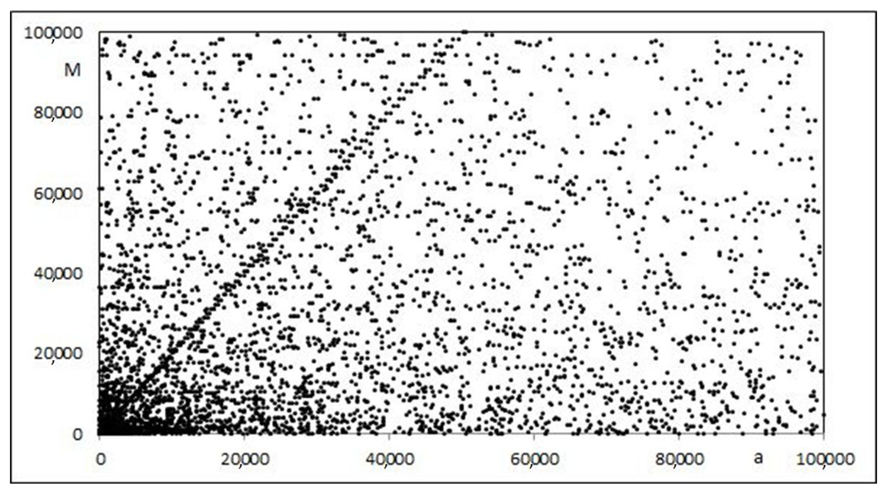
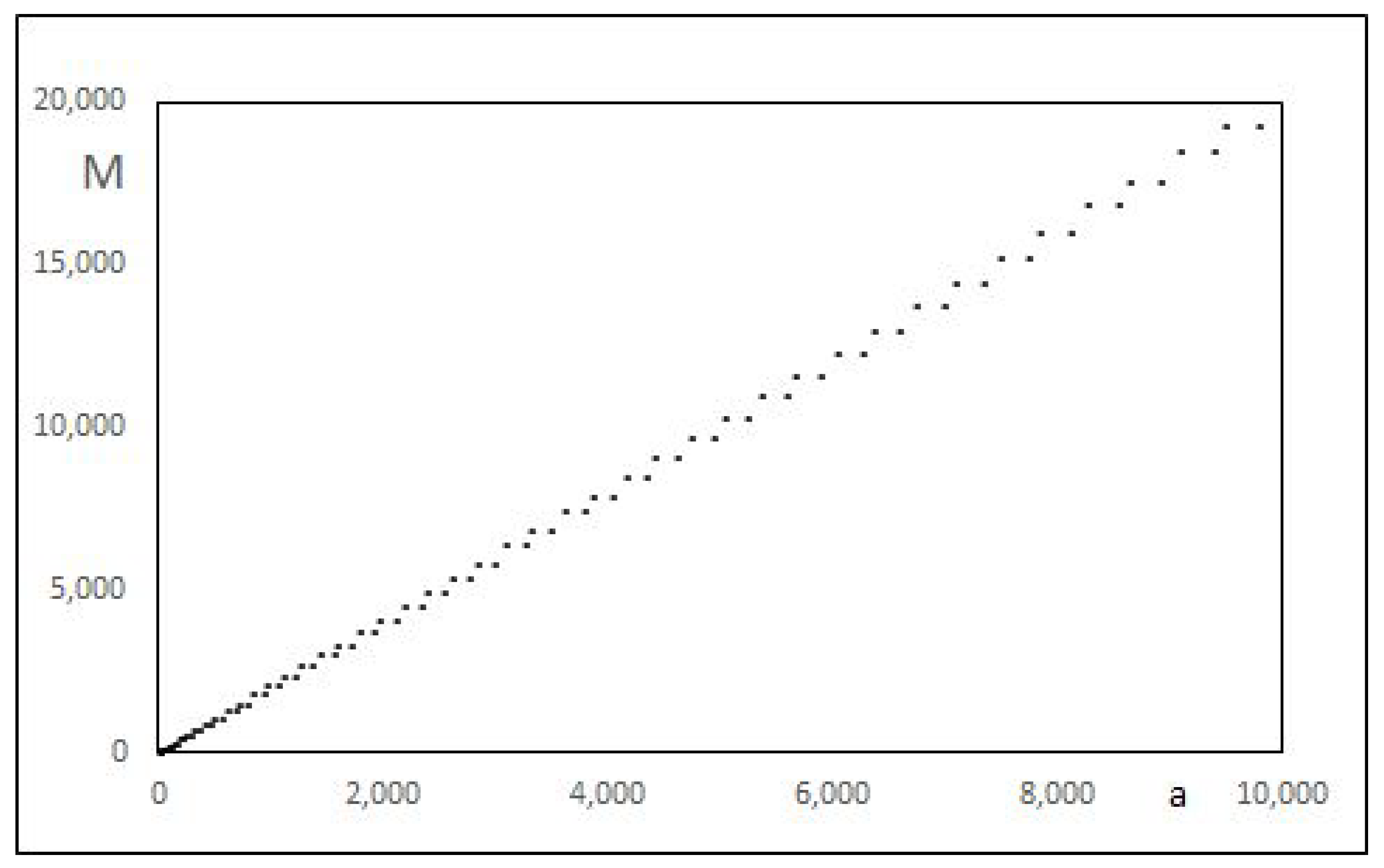
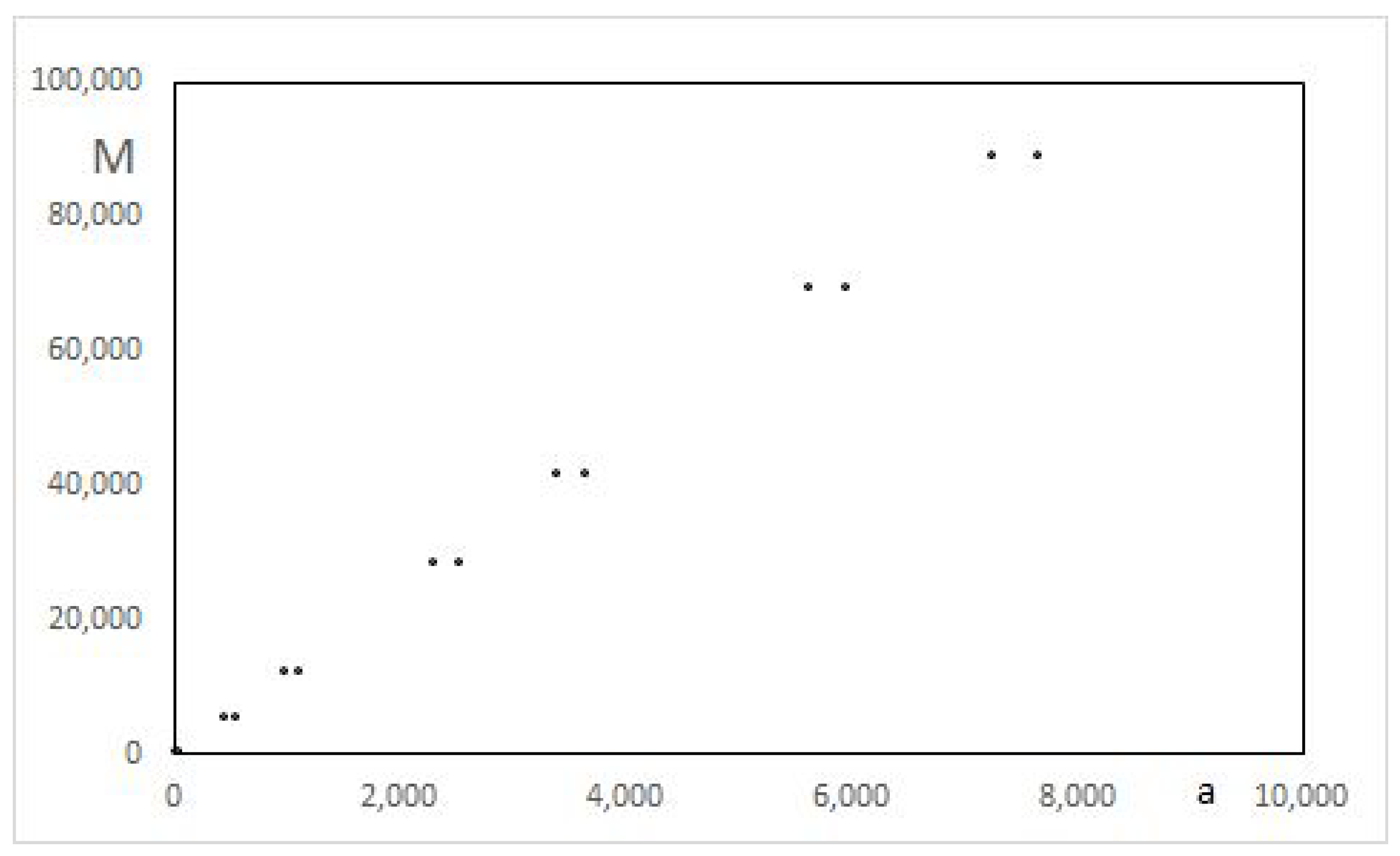
2.1. Observed Linear Features in the (a,M) Plot

For $M>1,a,i,s\in {\mathbb{Z}}^{*}$, the sum of M consecutive squared integers ${\left(a+i\right)}^2$ equaling a squared integer $s^2$ can be written [14] as

$$\sum _{i=0}^{M-1}{\left(a+i\right)}^2=M\left[{\left(a+\frac{M-1}{2}\right)}^2+\frac{M^2-1}{12}\right]$$

(2)

For $1\le a\le {10}^5$ and $2\le M\le {10}^5$, there are only 4078 couples of values of a and M among the approximately ${10}^{10}$ possibilities such that (2) holds. Figure 1 shows the distribution of these 4078 couples in an $\left(a,M\right)$ plot, where several groupings of interest are seen.

Figure 1. Distribution of M versus a for the 4078 couples $\left(a, M\right)$ found such as (2) holds, with $1\le a\le {10}^5$ and $2\le M\le {10}^5$.

The most visible is the grouping around a straight line of equation $M=2a+c$, where c is a constant, corresponding to a double infinite family of integers a. This grouping starts with the identity and the Pythagorean relations

$$\begin{array}{ccc}\hfill 0^2+1^2& =& 1^2\hfill \end{array}$$

(3)

$$\begin{array}{ccc}\hfill 3^2+4^2& =& 5^2\hfill \end{array}$$

(4)

for the same value of $M=2$ and, respectively, for $a=0$ and 3. This double infinite family has the property that couples of a values correspond to the same value of M. There are other similar groupings and double infinite families around straight lines of general equation $\mu M=2a+c_{\mu }$ for certain rational values of $\mu >0$, and where $c_{\mu }$ is a constant different for each value of $\mu$. Only groupings around inclined lines are considered, as the limit cases of $\mu =0$ and $\mu \to \infty$ corresponding to groupings around, respectively, vertical and horizontal lines are not treated here. The “horizontal” case for which one or several solutions in a exist for each value of M was investigated in [13,14].

2.2. Definition of Pairs and Theorem on Conditions on μ, M and a

Definition 1.

For $1\le j\le 2,M_{\mu ,k}>1,a_{j,\mu ,k}\in {\mathbb{Z}}^{*}$, for a given $\mu \in {\mathbb{Q}}^{+}$, two integers $a_{j,\mu ,k}$ are called a pair $\left(a_{1,\mu ,k},a_{2,\mu ,k}\right)$ if for the same value of $M_{\mu ,k}$ and $\forall k\in \mathbb{Z}$, the relations

$$\begin{array}{ccc}\hfill a_{1,\mu ,k}+a_{2,\mu ,k}& =& \mu M_{\mu ,k}+1\hfill \end{array}$$

(5)

$$\begin{array}{ccc}\hfill a_{2,\mu ,k}-a_{1,\mu ,k}& =& f_{\mu ,k}\hfill \end{array}$$

(6)

hold, where $f_{\mu ,k}=f_{\mu }\left(k\right)$ is a linear integer function of k for each value of μ, yielding

$$\mu M_{\mu ,k}=2a_{j,\mu ,k}\pm f_{\mu ,k}-1$$

(7)

where the upper or lower sign is taken for $j=1$ or 2.

The two families of $a_{1,\mu ,k}$ and $a_{2,\mu ,k}$ are characterized for each value of $\mu$ around the straight line of equation $\mu M=2a+c_{\mu }$ in the following theorem. However, relations (5) to (7) hold only for certain values of $M_{\mu ,k}$ and of $\mu$, called allowed values, which are determined further.

Theorem 1.

For $1\le j\le 2,i,\eta ,\delta ,M_{\mu ,k}>1,a_{j,\mu ,k}\in {\mathbb{Z}}^{*}$, $k,s_{j,\mu ,k}\in \mathbb{Z}$, for allowed values of $\mu \in {\mathbb{Q}}^{+}$, let $\mu =\left(\eta /\delta \right)$ be an irreducible fraction; if $\left(a_{1,\mu ,k},a_{2,\mu ,k}\right)$ is a pair of integers $a_{j,\mu ,k}$ for the same value of $M_{\mu ,k}$ and if

$$M_{\mu ,k}=\frac{\left(3f_{\mu ,k}^2-1\right)}{3{\left(\mu +1\right)}^2+1}=\frac{{\delta }^2\left(3f_{\mu ,k}^2-1\right)}{3{\left(\eta +\delta \right)}^2+{\delta }^2}$$

(8)

holds $\forall k\in \mathbb{Z}$, then the sums of squares of $M_{\mu ,k}$ consecutive integers $\left(a_{j,\mu ,k}+i\right)$ for $i=0$ to $M_{\mu ,k}-1$ are always equal to squared integers $s_{j,\mu ,k}^2$, with

$$\begin{array}{ccc}\hfill a_{j,\mu ,k}& =& \frac{1}{2\delta }\left(\eta M_{\mu ,k}+\delta \mp \sqrt{\frac{M_{\mu ,k}\left(3{\left(\eta +\delta \right)}^2+{\delta }^2\right)+{\delta }^2}{3}}\right)\hfill \end{array}$$

(9)

$$\begin{array}{ccc}\hfill s_{j,\mu ,k}& =& \frac{M_{\mu ,k}}{2\delta }\left(\sqrt{\frac{M_{\mu ,k}\left(3{\left(\eta +\delta \right)}^2+{\delta }^2\right)+{\delta }^2}{3}}\mp \left(\eta +\delta \right)\right)\hfill \end{array}$$

(10)

where the upper (respectively, lower) sign is taken for $j=1$ (respectively, 2).

Proof. 

Let $1\le j\le 2,i,\eta ,\delta ,M_{\mu ,k}>1,a_{j,\mu ,k}\in {\mathbb{Z}}^{*}$, $k,s_{j,\mu ,k}\in \mathbb{Z}$, $\mu =\left(\eta /\delta \right)\in {\mathbb{Q}}^{+}$ forming an irreducible fraction, i.e., $\gcd \left(\eta ,\delta \right)=1$. Let further $f_{\mu ,k}$ be a yet-unknown integer function of k for each value of $\mu$. Replacing in the second equality of (2) M by $M_{\mu ,k}$ and a by $a_{j,\mu ,k}$ from (7) yields, successively,

$$\begin{array}{ccc}\sum _{i=0}^{M_{\mu ,k}-1}{\left(a_{j,\mu ,k}+i\right)}^2& =& \frac{M_{\mu ,k}}{4}\left[{\left(2a_{j,\mu ,k}+M_{\mu ,k}-1\right)}^2+\frac{M_{\mu ,k}^2-1}{3}\right]\hfill \\ & =& \frac{M_{\mu ,k}}{4}\left[{\left(\left(\mu +1\right)M_{\mu ,k}\mp f_{\mu ,k}\right)}^2+\frac{M_{\mu ,k}^2-1}{3}\right]\hfill \\ & =& \frac{M_{\mu ,k}^2}{4}\left[\frac{\left(3{\left(\eta +\delta \right)}^2+{\delta }^2\right)M_{\mu ,k}}{3{\delta }^2}+\frac{3f_{\mu ,k}^2-1}{3M_{\mu ,k}}\right.\hfill \\ & & \mp 2\left(\frac{\eta +\delta }{\delta }\right)f_{\mu ,k}]\hfill \end{array}$$

(11)

where the upper (respectively, lower) sign in (11) is taken for $j=1$ (respectively, 2). For the expression between brackets in (11) to be a square, replace in (11) $f_{\mu ,k}$ by

$$f_{\mu ,k}=\sqrt{\frac{M_{\mu ,k}\left(3{\left(\eta +\delta \right)}^2+{\delta }^2\right)+{\delta }^2}{3{\delta }^2}}$$

(12)

from (8), immediately yielding (10). Replacing $f_{\mu ,k}$ (12) in (7) then yields (9). □

In addition, from Theorem 2, the following relations hold $\forall k\in \mathbb{Z}$

$$\begin{array}{ccc}\hfill a_{2,\mu ,k}-a_{1,\mu ,k}& =& \sqrt{\frac{M_{\mu ,k}\left(3{\left(\eta +\delta \right)}^2+{\delta }^2\right)+{\delta }^2}{3{\delta }^2}}\hfill \end{array}$$

(13)

$$\begin{array}{ccc}\hfill s_{2,\mu ,k}+s_{1,\mu ,k}& =& M_{\mu ,k}\sqrt{\frac{M_{\mu ,k}\left(3{\left(\eta +\delta \right)}^2+{\delta }^2\right)+{\delta }^2}{3{\delta }^2}}\hfill \end{array}$$

(14)

$$\begin{array}{ccc}& =& M_{\mu ,k}\left(a_{2,\mu ,k}-a_{1,\mu ,k}\right)\hfill \end{array}$$

(15)

$$\begin{array}{ccc}\hfill s_{2,\mu ,k}-s_{1,\mu ,k}& =& M_{\mu ,k}\left(\frac{\eta +\delta }{\delta }\right)\hfill \end{array}$$

(16)

$$\begin{array}{ccc}& =& a_{2,\mu ,k}+a_{1,\mu ,k}+M_{\mu ,k}-1\hfill \end{array}$$

(17)

2.3. Parametric Expressions of $f_{\mu ,k}$, $M_{\mu ,k}$, $a_{j,\mu ,k}$, $s_{j,\mu ,k}$

The above results hold only for certain values of $M_{\mu ,k}$ and of $\mu \in {\mathbb{Q}}^{+}$, which are called allowed values. They can be determined as follows. Relation (8) also reads

$${\left(\delta f_{\mu ,k}\right)}^2-M_{\mu ,k}{\left(\eta +\delta \right)}^2={\delta }^2\left(\frac{M_{\mu ,k}+1}{3}\right)$$

(18)

It was shown [15] that for (18) to hold:

-

$\delta \equiv 0\left(mod 6\right)$ and $\eta \equiv 1$ or $5\left(mod 6\right)$, $M_{\mu ,k}\equiv 0$ or $24\left(mod 72\right)$ and $M_{\mu ,k}\left(mod \left({\delta }^2/3\right)\right)\equiv 0$;

-

$\delta \equiv 1$ or $5\left(mod 6\right)$ and $\eta \equiv 1,3$ or $5\left(mod 6\right)$ and either $f_{\mu ,k}\equiv 1\left(mod 2\right)$ and $M_{\mu ,k}\equiv 2\left(mod 24\right)$ or $f_{\mu ,k}\equiv 0\left(mod 2\right)$ and $M_{\mu ,k}\equiv 11\left(mod 12\right)$, and $M_{\mu ,k}\left(mod {\delta }^2\right)\equiv 0$.

Parametric expressions of $f_{\mu ,k}$, $M_{\mu ,k}$, $a_{j,\mu ,k}$ and $s_{j,\mu ,k}$ as a function of $k\in \mathbb{Z}$, $\mu =\left(\eta /\delta \right)$ and initial values are found as follows.

Theorem 2.

For $1\le j\le 2,\eta ,\delta ,M_{\mu ,k}>1\in {\mathbb{Z}}^{+}$, $a_{j,\mu ,k}\in {\mathbb{Z}}^{*}$, $k,s_{j,\mu ,k}\in \mathbb{Z}$, $\mu ,\nu \in {\mathbb{Q}}^{+}$, for allowed values of $\mu =\left(\eta /\delta \right)$ and for pairs $\left(a_{1,\mu ,k},a_{2,\mu ,k}\right)$, $f_{\mu ,k}$ is a linear function of k, $M_{\mu ,k}$ and $a_{j,\mu ,k}$ are quadratic functions of k and $s_{j,\mu ,k}$ is a cubic function of k, as follows:

$$\begin{array}{ccc}\hfill f_{\mu ,k}& =& \left(3{\left(\eta +\delta \right)}^2+{\delta }^2\right)\nu k+f_{\mu ,0}\hfill \end{array}$$

(19)

$$\begin{array}{ccc}\hfill M_{\mu ,k}& =& 3{\delta }^2\left(3{\left(\eta +\delta \right)}^2+{\delta }^2\right){\nu }^2{k}^2+6{\delta }^2{f}_{\mu ,0}\nu k+M_{\mu ,0}\hfill \end{array}$$

(20)

$$\begin{array}{ccc}{a}_{j,\mu ,k}& =& \frac{1}{2}\left[3\eta \delta \left(3{\left(\eta +\delta \right)}^2+{\delta }^2\right){\nu }^2{k}^2+\left(6\eta \delta f_{\mu ,0}\mp \left(3{\left(\eta +\delta \right)}^2+{\delta }^2\right)\right)\nu k\right]\hfill \\ & & + a_{j,\mu ,0}\hfill \end{array}$$

(21)

$$\begin{array}{ccc}{s}_{j,\mu ,k}& =& \frac{1}{2}\left[3{\delta }^2{\left(3{\left(\eta +\delta \right)}^2+{\delta }^2\right)}^2{\nu }^3{k}^3\right.\hfill \\ & & + 3\delta \left(3{\left(\eta +\delta \right)}^2+{\delta }^2\right)\left(3\delta f_{\mu ,0}\mp \left(\eta +\delta \right)\right){\nu }^2{k}^2\hfill \\ & & \left.+\left({\left(3\delta f_{\mu ,0}\mp \left(\eta +\delta \right)\right)}^2-\left({\left(\eta +\delta \right)}^2+{\delta }^2\right)\right)\nu k\right]+s_{j,\mu ,0}\hfill \end{array}$$

(22)

where $\nu =1$ for $\delta \equiv 1$ or $5\left(mod 6\right)$, $\nu =\left(2/3\right)$ for $\delta \equiv 0\left(mod 6\right)$ and where the upper (respectively, lower) sign is taken for $j=1$ (respectively, 2).

Proof. 

For $1\le j\le 2,\eta ,\delta ,x,M_{\mu ,k}>1\in {\mathbb{Z}}^{+}$, $a_{j,\mu ,k}\in {\mathbb{Z}}^{*}$, $k,s_{j,\mu ,k}\in \mathbb{Z}$, $\mu ,\nu \in {\mathbb{Q}}^{+}$, for allowed values of $\mu =\left(\eta /\delta \right)$ and for pairs $\left(a_{1,\mu ,k},a_{2,\mu ,k}\right)$, let $f_{\mu ,k}$ (6) be a linear function of k, $f_{\mu ,k}=xk+f_{\mu ,0}$, where $f_{\mu ,0}=\left(a_{2,\mu ,0}-a_{1,\mu ,0}\right)$ is the initial value for $k=0$ of the difference (6) and x an integer function to be defined for some parameters. Then, (8) yields

$$\begin{array}{cc}{M}_{\mu ,k}& =\frac{{\delta }^2\left(3{\left(xk+f_{\mu ,0}\right)}^2-1\right)}{3{\left(\eta +\delta \right)}^2+{\delta }^2}\hfill \\ & =\frac{3{\delta }^{2}xk\left(xk+2f_{\mu ,0}\right)}{3{\left(\eta +\delta \right)}^2+{\delta }^2}+\frac{{\delta }^2\left(3f_{\mu ,0}^2-1\right)}{3{\left(\eta +\delta \right)}^2+{\delta }^2}\hfill \end{array}$$

(23)

The second term on the right of (23) is $M_{\mu ,0}$ by (8).

(i) If $\delta \equiv 1$ or $5\left(mod 6\right)$, as $M_{\mu ,k}\in {\mathbb{Z}}^{+}$, $\left(3{\left(\eta +\delta \right)}^2+{\delta }^2\right)$ must divide x in the first term of (23), then yielding (19) and (20) with $\nu =1$.

(ii) If $\delta \equiv 0\left(mod 6\right)$, simplifying the first term by 3, (23) reads

$$M_{\mu ,k}=\frac{{\delta }^{2}xk\left(xk+2f_{\mu ,0}\right)}{{\left(\eta +\delta \right)}^2+\left({\delta }^2/3\right)}+M_{\mu ,0}$$

(24)

As $M_{\mu ,k}\in {\mathbb{Z}}^{+}$, $\left({\left(\eta +\delta \right)}^2+\left({\delta }^2/3\right)\right)$ is a factor of x. However, as $\eta \equiv 1$ or $5\left(mod 6\right)$ for $\delta \equiv 0\left(mod 6\right)$, $\left({\left(\eta +\delta \right)}^2+\left({\delta }^2/3\right)\right)\equiv 1\left(mod 2\right)$ and as $f_{\mu ,k}\left(mod 2\right)\equiv f_{\mu ,0}\left(mod 2\right)$ $\forall k\in \mathbb{Z}$, x must be replaced by $2\left({\left(\eta +\delta \right)}^2+\left({\delta }^2/3\right)\right)$, then yielding (19) and (20) with $\nu =\left(2/3\right)$.

(iii) Further, replacing $f_{\mu ,k}$ and $M_{\mu ,k}$ by (19) and (20) in $a_{j,\mu ,k}$ from (7) and in $s_{j,\mu ,k}$ (10) with (12) yields directly (21) and (22) with the upper (or lower) sign for $j=1$ (or 2). □

2.4. Finding Allowed Values of $\mu =\left(\eta /\delta \right)$ and $M_{\mu ,k}$

Finding the allowed values of $\mu =\left(\eta /\delta \right)$, $M_{\mu ,0}$ and $f_{\mu ,0}$ requires solving the generalized Pell Equation (18) for $k=0$ in variables $\left(\delta f_{\mu ,0}\right)$ and $\left(\eta +\delta \right)$.

In general, for $X,Y,D,N,x_f,y_f,n\in {\mathbb{Z}}^{+}$ and D square-free (i.e., $\sqrt{D}\notin \mathbb{Z}$), a generalized Pell equation $X^2-D{Y}^2=N$ admits either no solution or one or several fundamental solution(s) $\left(X_1,Y_1\right)$ and also one or several infinite branches of solutions $\left(X_n,Y_n\right)$. Several methods exist to find the fundamental solutions of the generalized Pell equation (see [16,17,18]). Two methods are used further: first, a brute-force search method, i.e., trying several values of Y until the smallest $X_1=\sqrt{N+D{Y}_1^2}\in {\mathbb{Z}}^{+}$ is found; second, Matthews’ method [19] based on an algorithm by Frattini [20,21,22] using Nagell’s bounds [23,24]. Once fundamental solution(s) $\left(X_1,Y_1\right)$ have been found one way or another, noting $\left(x_f,y_f\right)$, the fundamental solutions of the related simple Pell equation $X^2-D{Y}^2=1$, the other solutions $\left(X_n,Y_n\right)$ can be found by

$$X_n+\sqrt{D}{Y}_n=\pm \left(X_1+\sqrt{D}{Y}_1\right){\left(x_f+\sqrt{D}{y}_f\right)}^n$$

(25)

for a proper choice of sign ± [25], which can also be written as a function of Chebyshev’s polynomials [14]

$$\begin{array}{ccc}\hfill X_n& =& X_1{T}_{n-1}\left(x_f\right)+D{Y}_1{y}_f{U}_{n-2}\left(x_f\right)\hfill \end{array}$$

(26)

$$\begin{array}{ccc}\hfill Y_n& =& X_1{y}_f{U}_{n-2}\left(x_f\right)+Y_1{T}_{n-1}\left(x_f\right)\hfill \end{array}$$

(27)

where $T_{n-1}\left(x_f\right)$ and $U_{n-2}\left(x_f\right)$ are Chebyshev polynomials of the first and second kinds evaluated at $x_f$.

The generalized Pell Equation (18) can be written as

$${\left(\lambda f_{\mu ,0}\right)}^2-\left(\frac{{\lambda }^2{M}_{\mu ,0}}{{\delta }^2}\right){\left(\eta +\delta \right)}^2=\frac{{\lambda }^2\left(M_{\mu ,0}+1\right)}{3}$$

(28)

with $X=\lambda f_{\mu ,0}$, $Y=\left(\eta +\delta \right)$, $D=\left({\lambda }^2{M}_{\mu ,0}/{\delta }^2\right)$ and $N={\lambda }^2\left(M_{\mu ,0}+1\right)/3$, and where $\lambda =1$ if $\delta \equiv 1$ or $5\left(mod 6\right)$ and $\lambda =3$ if $\delta \equiv 0\left(mod 6\right)$.

To use Matthews’ method [19], the parameters D and N must be fixed with values of $\delta$ and $M_{\mu ,0}$ that can be chosen from the allowed congruent values (see Section 2.3) and be tried one by one until fundamental solutions are found. Alternatively, fixing the values of $\eta$ and $\delta$, a brute-force search method can be used to find $f_{\mu ,0}\in {\mathbb{Z}}^{+}$ for the smallest value of $M_{\mu ,0}\in {\mathbb{Z}}^{+}$, with, from (12),

$$f_{\mu ,0}=\sqrt{\frac{M_{\mu ,0}\left(3{\left(\eta +\delta \right)}^2+{\delta }^2\right)+{\delta }^2}{3{\delta }^2}}$$

(29)

Relation (29) then yields the allowed values of $\mu ,M_{\mu ,0}$ and $f_{\mu ,0}$ given in Table 1 for $\delta =1,$ $\mu =\eta \in {\mathbb{Z}}^{+}$, for $0\le \mu \le 100$ ([26] gives all values of $\left(\mu +1\right)$ such that $\left(3{\left(\mu +1\right)}^2+1\right)$ is prime, for which (29) holds.) and in [27] for $\delta \ne 1,$$\mu =\left(\eta /\delta \right)\in {\mathbb{Q}}^{+}$, for $0<\eta ,\delta \le 100$.

Table 1. Values of $M_{\mu ,0}$ and $f_{\mu ,0}$ for $0\le \mu \le 100$.

$\mathit{\mu }$	${\mathit{M}}_{\mathit{\mu },0}$	${\mathit{f}}_{\mathit{\mu },0}$	$\mathit{\mu }$	${\mathit{M}}_{\mathit{\mu },0}$	${\mathit{f}}_{\mathit{\mu },0}$	$\mathit{\mu }$	${\mathit{M}}_{\mathit{\mu },0}$	${\mathit{f}}_{\mathit{\mu },0}$
1	2	3	29	26	153	63	3263	3656
5	11	20	33	299	588	67	9563	6650
7	74	69	35	479	788	69	2	99
11	2	17	39	1391	1492	77	74	671
15	194	223	43	59	338	81	1202	2843
19	122	221	49	491	1108	83	146	1015
21	983	690	53	1739	2252	85	1874	3723
25	506	585	55	383	1096	97	23	470
27	47	192	57	2327	2798

Once a set of values has been found for $\eta ,\delta ,M_{\mu ,0}$ and $f_{\mu ,0}$ as fundamental solution(s) of the generalized Pell Equation (28), other allowed values for $\eta$ and $f_{\mu ,0}$ can be found from the other solutions of (28) using the values of $\delta$ and $M_{\mu ,0}$ with (26) and (27), written as

$$\begin{array}{ccc}\hfill f_{{\mu }_n,0}& =& f_{{\mu }_1,0}{T}_{n-1}\left(x_f\right)+\left(\frac{\lambda M_{\mu ,0}}{{\delta }^2}\right)\left({\eta }_1+\delta \right)y_f{U}_{n-2}\left(x_f\right)\hfill \end{array}$$

(30)

$$\begin{array}{ccc}\hfill {\eta }_n& =& \lambda f_{{\mu }_1,0}{y}_f{U}_{n-2}\left(x_f\right)+\left({\eta }_1+\delta \right)T_{n-1}\left(x_f\right)-\delta \hfill \end{array}$$

(31)

3. Results and Discussion

To demonstrate the soundness of the method exposed above using the Pell equation approach, we give here several examples.

Example 1.

For $\delta =1$ and $\mu =\eta =1$, $M_{1,0}=2$ and $f_{1,0}=3$ from Table 1. Using $M_{1,0}$ and δ as constants in (28) with $\lambda =1$, it reduces to a simple Pell equation $f_{\mu ,0}^2-2{\left(\mu +1\right)}^2=1$ (see, e.g., [28,29,30,31]) that admits the single fundamental solution $\left(X_1,Y_1\right)=\left(f_{{\mu }_1,0},\left({\mu }_1+1\right)\right)=\left(3,2\right)$ or $\left(f_{{\mu }_1,0},{\mu }_1\right)=\left(3,1\right)$ and an infinity of other solutions that can be found $\forall n\in {\mathbb{Z}}^{+}$ by

$$\begin{array}{ccc}\hfill f_{{\mu }_n,0}& =& \frac{{\left(3+2\sqrt{2}\right)}^n+{\left(3-2\sqrt{2}\right)}^n}{2}=3,17,99,577,3363,\dots \hfill \end{array}$$

(32)

$$\begin{array}{ccc}\hfill {\mu }_n& =& \frac{{\left(3+2\sqrt{2}\right)}^n-{\left(3-2\sqrt{2}\right)}^n}{2\sqrt{2}}-1=1,11,69,407,2377,\dots \hfill \end{array}$$

(33)

where ${\mu }_n$ are the Pell numbers [32] of even indices minus one. These new values of $\left(f_{{\mu }_n,0},{\mu }_n\right)$ for $n>1$ define new groupings around straight lines of general equation ${\mu }_{n}M=2a+c_{{\mu }_n}$, with the initial value $M_{{\mu }_n,0}=2$.

• For $\delta =1$, $\eta =1$, i.e., $\mu =1$, $M_{1,0}=2$, $f_{1,0}=3$, $\nu =1$, (20) to (22) yield
• $M_{1,k}=39k^2+18k+2$,
• $a_{1,1,k}=\left(39k^2+5k\right)/2$, $a_{2,1,k}=\left(39k^2+31k+6\right)/2$,
• $s_{1,1,k}=\left(507k^3+273k^2+44k+2\right)/2$, $s_{2,1,k}=\left(507k^3+429k^2+116k+10\right)/2$,
• and values of $M_{\mu ,k}$, $a_{1,\mu ,k}$ and $a_{2,\mu ,k}$ for $-10\le k\le 10$ are given in Table 2.

Table 2. Values of $M_{\mu ,k}$, $a_{1,\mu ,k}$, $a_{2,\mu ,k}$ for $\mu =1,5,\left(1/6\right)$ and $-10\le k\le 10$.

	$\mathit{\mu }=1$			$\mathit{\mu }=5$			$\mathit{\mu }=1/6$
k	$M_{1,k}$	$a_{1,1,k}$	$a_{2,1,k}$	$M_{5,k}$	$a_{1,5,k}$	$a_{2,5,k}$	$M_{1/6,k}$	$a_{1,1/6,k}$	$a_{2,1/6,k}$
0	2	0	3	11	18	38	312	15	38
−1	23	17	7	218	590	501	5784	532	433
1	59	22	38	458	1081	1210	12408	962	1107
−2	122	73	50	1079	2797	2599	28824	2513	2292
2	194	83	112	1559	3779	4017	42072	3373	3640
−3	299	168	132	2594	6639	6332	69432	5958	5615
3	407	183	225	3314	8112	8459	89304	7248	7637
−4	554	302	253	4763	12116	11700	127608	10867	10402
4	698	322	377	5723	14080	14536	154104	12587	13098
−5	887	475	413	7586	19228	18703	203352	17240	16653
5	1067	500	568	8786	21683	22248	236472	19390	20023
−6	1298	687	612	11063	27975	27341	296664	25077	24368
6	1514	717	798	12503	30921	31595	336408	27657	28412
−7	1787	938	850	15194	38357	37614	407544	34378	33547
7	2039	973	1067	16874	41794	42577	453912	37388	38265
−8	2354	1228	1127	19979	50374	49522	535992	45143	44190
8	2642	1268	1375	21899	54302	55194	588984	48583	49582
−9	2999	1557	1443	25418	64026	63065	682008	57372	56297
9	3323	1602	1722	27578	68445	69446	741624	61242	62363
−10	3722	1925	1798	31511	79313	78243	845592	71065	69868
10	4082	1975	2108	33911	84223	85333	911832	75365	76608

Figure 2 shows the distribution of M versus a for $\mu =1$.

Figure 2. Distribution of M versus a for $\mu =1$.

Example 2.

For $\delta =1$ and $\mu =\eta =5$, $M_{5,0}=11$ and $f_{5,0}=20$ from Table 1. Using $M_{5,0}$ and δ as constants in (28) with $\lambda =1$ yields the generalized Pell equation $f_{\mu ,0}^2-11{\left(\mu +1\right)}^2=4$. Using Matthews’ method [19] yields the single fundamental solution $\left(f_{{\mu }_1,0},\left({\mu }_1+1\right)\right)=\left(2,0\right)$, which is of no use. However, as the right-hand term is a squared integer, the equation can be rewritten as a simple Pell equation ${\left(f_{\mu ,0}/2\right)}^2-11{\left(\left(\mu +1\right)/2\right)}^2=1$, which admits the fundamental solution $\left(\left(f_{{\mu }_1,0}/2\right),\left(\left({\mu }_1+1\right)/2\right)\right)=\left(10,3\right)$ or $\left(f_{{\mu }_1,0},{\mu }_1\right)=\left(20,5\right)$ and an infinity of other solutions $\forall n\in {\mathbb{Z}}^{+}$

$$\begin{array}{ccc}\hfill f_{{\mu }_n,0}& =& {\left(10+3\sqrt{11}\right)}^n+{\left(10-3\sqrt{11}\right)}^n=20,398,7940,158402,\dots \hfill \end{array}$$

(34)

$$\begin{array}{ccc}\hfill {\mu }_n& =& \frac{{\left(10+3\sqrt{11}\right)}^n-{\left(10-3\sqrt{11}\right)}^n}{\sqrt{11}}-1=5,119,2393,47759,\dots \hfill \end{array}$$

(35)

• For $\delta =1$, $\eta =5$, i.e., $\mu =5$, $M_{5,0}=11$, $f_{5,0}=20$, $\nu =1$, (20) to (22) yield (see Table 2)
• $M_{5,k}=327k^2+120k+11$,
• $a_{1,5,k}=\left(1635k^2+491k+36\right)/2$, $a_{2,5,k}=\left(1635k^2+709k+76\right)/2$,
• $s_{1,5,k}=\left(35643k^3+17658k^2+2879k+154\right)/2$,
• $s_{2,5,k}=\left(35643k^3+21582k^2+4319k+286\right)/2$.

Figure 3 shows the distribution of M versus a for $\mu =5$.

Figure 3. Distribution of M versus a for $\mu =5$.

Example 3.

For $\eta =1$ and $\delta =6$, i.e., $\mu =1/6$, $M_{1/6,0}=312$ and $f_{1/6,0}=23$ [27]. Using $M_{1/6,0}$ and δ as constants in (28) with $\lambda =3$ yields ${\left(3f_{\mu ,0}\right)}^2-78{\left(\eta +6\right)}^2=939$, which, by [19], has two fundamental solutions $\left(\left(3f_{{\mu }_1,0}\right),\left({\eta }_1+6\right)\right)=\left(69,7\right)$ and $\left(381,43\right)$, yielding $\left(f_{{\mu }_1,0},{\eta }_1\right)=\left(23,1\right)$ and $\left(127,37\right)$, respectively. The fundamental solutions of the related simple Pell equation $X^2-78Y^2=1$ are $\left(x_f,y_f\right)=\left(53,6\right)$. Other values of $\left(f_{{\mu }_n,0},{\eta }_n\right)$ can be found on the two infinite branches corresponding to these two fundamental solutions by (30) and (31) as

$$\begin{array}{ccc}\hfill f_{{\mu }_n,0}& =& 23T_{n-1}\left(53\right)+1092U_{n-2}\left(53\right)\hfill \end{array}$$

(36)

$$\begin{array}{ccc}& =& 23,2311,244943,25961647,2751689639,\dots \hfill \end{array}$$

(37)

$$\begin{array}{ccc}\hfill {\eta }_n& =& 414U_{n-2}\left(53\right)+7T_{n-1}\left(53\right)-6\hfill \end{array}$$

(38)

$$\begin{array}{ccc}& =& 1,779,83197,8818727,934702489,\dots \hfill \end{array}$$

(39)

for the first fundamental solution and

$$\begin{array}{ccc}\hfill f_{{\mu }_n,0}& =& 127T_{n-1}\left(53\right)+6708U_{n-2}\left(53\right)\hfill \end{array}$$

(40)

$$\begin{array}{ccc}& =& 127,13439,1424407,150973703,16001788111,\dots \hfill \end{array}$$

(41)

$$\begin{array}{ccc}\hfill {\eta }_n& =& 2286U_{n-2}\left(53\right)+43T_{n-1}\left(53\right)-6\hfill \end{array}$$

(42)

$$\begin{array}{ccc}& =& 37,4559,483841,51283211,5435537149,\dots \hfill \end{array}$$

(43)

for the second fundamental solution. For $\eta =1$, $\delta =6$, i.e., $\mu =1/6$, $M_{1/6,0}=312$, $f_{1/6,0}=23$, $\nu =\left(2/3\right)$, (20) to (22) yield (see Table 2).

• $M_{1/6,k}=8784k^2+3312k+312$,
• $a_{1,1/6,k}=732k^2+215k+15$, $a_{2,1/6,k}=732k^2+337k+38$,
• $s_{1,1/6,k}=535824k^3+297924k^2+55188k+3406$,
• $s_{2,1/6,k}=535824k^3+308172k^2+59052k+3770$.

Figure 4 shows the distribution of M versus a for $\mu =1/6$.

Figure 4. Distribution of M versus a for $\mu =1/6$.

4. Conclusions

Definition 1 and Theorem 2 allowed us to show that regular linear features exist in the distribution of couples of values a and M in the $\left(a,M\right)$ plot, where $a^2$ and M are the first term and the number of terms in sums of consecutive squared integers equal to integer squares. These regular features correspond to groupings of pairs of a values for successive same values of M found on either side of straight lines of equation $\mu M=2a+c$ for positive rational values of $\mu =\left(\eta /\delta \right)$ and where c is a constant.

For allowed values of $\eta$ and $\delta$ such as $\eta \equiv 1\left(mod 2\right)$ and $\delta \equiv 0,1$ or $5\left(mod 6\right)$, if $M_{\mu ,k}={\delta }^2\left(3{\left(a_{2,\mu ,k}-a_{1,\mu ,k}\right)}^2-1\right)/\left(3{\left(\eta +\delta \right)}^2+{\delta }^2\right)$ holds $\forall k\in \mathbb{Z}$ and for pairs $\left(a_{1,\mu ,k},a_{2,\mu ,k}\right)$, then the sums of $M_{\mu ,k}$ consecutive squared integers starting with $a_{1,\mu ,k}$ or $a_{2,\mu ,k}$ are always equal to squared integers $s_{1,\mu ,k}^2$ or $s_{2,\mu ,k}^2$$\forall k\in \mathbb{Z}$. Parametric equations are found as a function of $k\in \mathbb{Z}$: linear for $f_{\mu ,k}=\left(a_{2,\mu ,k}-a_{1,\mu ,k}\right)$, quadratic for $M_{\mu ,k}$, $a_{1,\mu ,k}$ and $a_{2,\mu ,k}$ and cubic for $s_{1,\mu ,k}$ and $s_{2,\mu ,k}$.

The allowed values of $\eta ,\delta ,M_{\mu ,0}$ and of the difference $f_{\mu ,0}=a_{2,\mu ,0}-a_{1,\mu ,0}$ are found by solving the generalized Pell equation ${\left(\delta f_{\mu ,0}\right)}^2-M_{\mu ,0}{\left(\eta +\delta \right)}^2={\delta }^2\left(M_{\mu ,0}+1\right)/3$ and further allowed values of ${\eta }_n$ and $f_{{\mu }_n,0}$ can be calculated for fixed values of $\delta$ and $M_{\mu ,0}$ using Chebyshev polynomials.

This approach allows us to completely solve the classical problem of the sums of consecutive squared integers equal to squared integers and provide all solutions in infinite families.

References

1. Lucas, E. Recherches sur l’analyse Indéterminée et l’arithmétique de Diophante; C. Desrosiers: Moulins, France, 1873; p. 90. Available online: http://edouardlucas.free.fr/pdf/oeuvres/diophante.pdf (accessed on 25 January 2024).
2. Lucas, E. Question 1180. Nouv. Ann. Math. 1875, 14, 336. [Google Scholar]
3. Moret-Blanc, M. Question 1180. Nouv. Ann. Math. 1876, 15, 46–48. [Google Scholar]
4. Lucas, E. Solution de la Question 1180. Nouv. Ann. Math. 1877, 15, 429–432. [Google Scholar]
5. Watson, G.N. The Problem of the Square Pyramid. Messenger Math. 1918, 48, 1–22. [Google Scholar]
6. Ljunggren, W. New solution of a problem proposed by E. Lucas. Norsk Mat. Tid. 1952, 34, 65–72. [Google Scholar]
7. Ma, D.G. An Elementary Proof of the Solutions to the Diophantine Equation 6y2 = x(x + 1)(2x + 1). Sichuan Daxue Xuebao 1985, 4, 107–116. [Google Scholar]
8. Anglin, W.S. The Square Pyramid Puzzle. Am. Math. Mon. 1990, 97, 120–124. [Google Scholar] [CrossRef]
9. Alfred, U. Consecutive integers whose sum of squares is a perfect square. Math. Mag. 1964, 37, 19–32. [Google Scholar] [CrossRef]
10. Philipp, S. Note on consecutive integers whose sum of squares is a perfect square. Math. Mag. 1964, 37, 218–220. [Google Scholar] [CrossRef]
11. Laub, M. Squares Expressible as a Sum of n Consecutive Squares, Advanced Problem 6552. Am. Math. Mon. 1990, 97, 622–625. [Google Scholar] [CrossRef]
12. Beeckmans, L. Squares Expressible as Sum of Consecutive Squares. Am. Math. Mon. 1994, 101, 437–442. [Google Scholar] [CrossRef]
13. Pletser, V. Congruence conditions on the number of terms in sums of consecutive squared integers equal to squared integers. arXiv 2014, arXiv:1409.7969. [Google Scholar] [CrossRef]
14. Pletser, V. Finding all squared integers expressible as the sum of consecutive squared integers using generalized Pell equation solutions with Chebyshev polynomials. arXiv 2014, arXiv:1409.7972. [Google Scholar] [CrossRef]
15. Pletser, V. Congruent conditions on the number of terms, on the ratio number of terms to first terms and on the difference of first terms for sums of consecutive squared integers equal to squared integers. arXiv 2014, arXiv:1410.0727. [Google Scholar] [CrossRef]
16. Matthews, K.R. The Diophantine Equation x2Dy2 = N, D > 0, in integers. Expo. Math. 2000, 18, 323–331. [Google Scholar]
17. Mollin, R.A. Fundamental Number Theory with Applications; CRC Press: New York, NY, USA, 1998; pp. 294–307. [Google Scholar]
18. Robertson, J.P. Solving the Generalized Pell Equation X2DY2 = N. 2004. Available online: https://studylib.net/doc/18752934/solving-281 (accessed on 28 December 2023).
19. Matthews, K. Quadratic Diophantine Equations BCMATH Programs. Available online: http://www.numbertheory.org/php/main_pell.html (accessed on 28 December 2023).
20. Frattini, G. Dell’analisi indeterminata di secondo grado. Period. Mat. 1891, 6, 169–180. [Google Scholar]
21. Frattini, G. A complemento di alcuni teore mi del sig. Tchebicheff Rom. Acc. L. Rend. 1892, 5, 85–91. [Google Scholar]
22. Frattini, G. Dell’analisi indeterminata di secondo grado. Periodico di Mat. 1892, 7, 172–177. [Google Scholar]
23. Matthews, K.; Robertson, J. On the Converse of a Theorem of Nagell and Tchebicheff. Available online: http://www.numbertheory.org/PDFS/nagell2.pdf (accessed on 28 December 2023).
24. Nagell, T. Introduction to Number Theory; Wiley: New York, NY, USA, 1951; pp. 195–212. [Google Scholar]
25. Matthews, K. The Diophantine Equation x2Dy2 = N. Available online: http://www.numbertheory.org/PDFS/patz5.pdf (accessed on 28 December 2023).
26. Nambi, P. Numbers n such that 3*n⌃2 + 1 is prime, Sequence A111051 in The On-line Encyclopedia of Integer Sequences. Available online: https://oeis.org/A111051 (accessed on 28 December 2023).
27. Pletser, V. Fundamental Solutions of the Generalized Pell Equation (δf)2M(η + δ)2 = δ2(M + 1)/3 for 0 < η, δ < 100. Res. Gate. 2014. Available online: https://www.researchgate.net/publication/264496057_Fundamental_solutions_of_the_generalized_Pell_equation_%28f%292-M%28%292_2%28M1%293_for_0__100?ev=prf_pub (accessed on 7 August 2014).
28. Lagrange, J.L. Solution d’un Probleme d’Arithmetique, in Oeuvres de Lagrange; Serret, J.-A., Ed.; Gauthier-Villars: Paris, France, 1867; Volume 1, pp. 671–731. [Google Scholar]
29. Lenstra, H.W., Jr. Solving the Pell Equation. Not. Ams. 2002, 49, 182–192. [Google Scholar]
30. O’Connor, J.J.; Robertson, E.F. Pell’s Equation, JOC/EFR February 2002. Available online: https://mathshistory.st-andrews.ac.uk/HistTopics/Pell/ (accessed on 28 December 2023).
31. Pletser, V. On continued fraction development of quadratic irrationals having all periodic terms but last equal and associated general solutions of the Pell equation. J. Number Theory 2013, 136, 339–353. [Google Scholar] [CrossRef]
32. Sloane, N.J.A. Pell Numbers, Sequence A000129 in The On-line Encyclopedia of Integer Sequences. Available online: https://oeis.org/A000129 (accessed on 28 December 2023).
Disclaimer/Publisher’s Note: The statements, opinions and data contained in all publications are solely those of the individual author(s) and contributor(s) and not of MDPI and/or the editor(s). MDPI and/or the editor(s) disclaim responsibility for any injury to people or property resulting from any ideas, methods, instructions or products referred to in the content.
Article Metrics
Citations
Article Access Statistics
Multiple requests from the same IP address are counted as one view.