Characterization of Dual Spacelike Curves on Dual Lightlike Cone ${\stackrel{\mathbf{~}}{\mathit{Q}}}^{\mathbf{2}}$ Utilizing the Structure Function

Abstract

This study is about the dual spacelike curves lying on the dual lightlike cone, which can be either symmetric or asymmetric. We first establish the dual associated curve, which is related to the reference curve. Using these curves and the derivative of the reference curve, we derive the dual asymptotic orthonormal frame. Next, we define the dual structure function, curvature function, and Frenet formulae, and express the curvature function in terms of the dual structure function. This leads to a differential equation that characterizes the dual cone curve in relation to its curvature function. Since curves with constant curvature maintain the same curvature at every point, their geometry is more predictable. Therefore, we assume that the dual cone curvature function is constant and examine how this condition affects the behavior and geometric properties of the dual curves. As a result of this investigation, some new results and definitions are obtained.

1. Introduction

Curves are essential geometric structures with broad applications across numerous fields including architecture, cartography, military technology, physics, and astronomy. In geometry, specific types of curves, such as Bezier, B-spline, spherical, and associated curves, serve specialized roles in Euclidean, Lorentzian, dual, and dual Lorentzian spaces. Bezier and B-spline curves, for instance, are pivotal in computer graphics and CAD for rendering smooth, precise forms; whereas spherical curves are critical in navigation and cartography, representing the shortest paths on spherical surfaces. Evolutes and involutes, which are types of associated curves, are integral in gear design to maintain constant velocity ratios. Beyond Euclidean space, studies of curves in Lorentzian geometry contribute to relativistic physics by modeling particle trajectories in spacetime. Thus, curves are indispensable tools that bridge theoretical frameworks and practical applications across various scientific and engineering domains.

Numerous studies examine various types of curves within distinct geometric spaces. Bonnor [1] introduced the Cartan frame, emphasizing its utility in the study of null curves. Ferrandez and Gimenez [2] extended the Cartan frame concept to Lorentzian space forms. Kılıç and Karadağ [3] investigate null curves on ruled surfaces in Minkowski 3-space, providing the definition of the quasi-Darboux vector. Liu [4] studied curves in the lightlike cone and gave an asymptotic frame field along the curve and defined cone curvature functions for this frame field. Study [5] showed that curves on the light cone can be spacelike or lightlike. Finally, Liu and Meng [6] derived representation formulae for spacelike curves on the two- and three-dimensional light cones by using structure functions and utlilized them to analyze the properties of these curves. There are also other studies on the curves on a lightlike cone [7,8,9,10,11,12]. In addition to studies on curves in Lorentzian space, there have also been studies on surfaces and surface characterizations in Lorentzian space [12,13,14,15,16]. There is a transformation between the lines of the real vector space and the points of the dual vector space that is called e-study transformation. And this transformation is defined between the lines of the Lorentzian space and points of the dual Lorentzian space. Therefore, since relationships can be established between surfaces and curves in these spaces, studies have also been conducted in the dual spaces and the dual Lorentzian spaces [17,18,19,20].

Despite these advancements, further exploration of the curves in the dual Lorentzian spaces remains necessary. This study aims to address this gap by providing a detailed analysis of the dual spacelike curves on the dual lightlike cone, defined by the arc parameter of the real indicatrix. We introduce the dual asymptotic frame, Frenet derivative formulae, and the cone curvature function of these curves. Additionally, the dual lightlike curve, drawn on the dual lightlike cone by the third component of the frame, is defined as the dual associated curve. By examining the dual quasi-Darboux vector of the curve, we establish the relationship between the dual cone curvature function and the dual quasi-Darboux vector. We define the dual structure function of the curve and derive its representation using this structure function. Based on this, we formulate a differential equation characterizing the curve in terms of the dual cone curvature function. This equation is then solved for special cases, leading to various characterizations of these curves. Some examples related to the topic are provided. However, the question of whether the curve is symmetric or asymmetric remains open. This paper is organized into three main sections: the first section introduces the fundamental concepts; the second section presents the detailed analysis of dual spacelike curves; and the third section summarizes the main findings and outlines potential directions for future research.

2. Preliminaries

$IR$ is the standard notation for the field of real numbers, representing a one-dimensional vector space.

$I{R}^3$ denotes the three-dimensional real vector space consisting of ordered triples of real numbers.

Lorentzian space $I{R}_1^3$ is the vector space $I{R}^3$ provided with the following Lorentzian inner product:

$$〈\mathit{a},\mathit{a}〉=-a_1{b}_1+a_2{b}_2+a_3{b}_3,$$

where, $\mathit{a}=(a_1,a_2,a_3)$ and $\mathit{b}=(b_1,b_2,b_3)\in I{R}_1^3$.

A vector $\mathit{a}=(a_1,a_2,a_3)$ of $I{R}_1^3$ is classified as one of the following:

• Timelike if it satisfies $〈\mathit{a},\mathit{a}〉<0$;
• Spacelike if it satisfies $〈\mathit{a},\mathit{a}〉>0$ or $\mathit{a}=0$;
• Lightlike (null) if it satisfies $〈\mathit{a},\mathit{a}〉=0$ and $\mathit{a}\ne 0$.

Similarly, an arbitrary curve $\alpha (s)$ in $I{R}_1^3$ is classified as spacelike, timelike, or lightlike (null) if all its velocity vectors are spacelike, timelike, or lightlike (null), respectively [12]. The norm of a vector $\mathit{a}$ is defined by $‖\mathit{a}‖=\sqrt{\left|〈\mathit{a},\mathit{a}〉\right|}$. Now, let $\mathit{a}=(a_1,a_2,a_3)$ and $\mathit{b}=(b_1,b_2,b_3)$ present two vectors in $I{R}_1^3$.

The Lorentzian cross product of $\mathit{a}$ and $\mathit{b}$ is expressed as

$$\mathit{a}\times \mathit{b}=(a_2{b}_3-a_3{b}_2,a_1{b}_3-a_3{b}_1,a_2{b}_1-a_1{b}_2).$$

By using this definition, it can be easily shown that $〈\mathit{a}\times \mathit{b},\mathit{c}〉=det(\mathit{a},\mathit{b},\mathit{c})$ [12,21].

The set of lightlike vectors is referred to as the lightlike cone, indicated by [4]

$$Q^2=\left\{\mathit{a}=(a_1, a_2, a_3)\in I{R}_1^3: 〈\mathit{a},\mathit{a}〉=0\right\}.$$

Here, $\overline{a}=a+\epsilon a^{*}$ is called the dual number and $\epsilon$ is called the dual unit. The set of dual numbers is given by

$$ID=\left\{\overline{a}=a+\epsilon a^{\ast }: a,a^{\ast }\in IR, {\epsilon }^2=0\right\}.$$

The dual function of dual numbers establishes a mapping of the dual number space onto itself. The characteristics of dual functions were extensively examined by Velkamp [22]. He formulated the general expression for dual analytic (differentiable) functions as follows:

$$f(\overline{x})=f(x)+\epsilon x^{*}{f}^{\prime }(x),$$

where $f^{\prime }(x)$ is a derivative of $f(x)$ and $x,x^{*}\in IR$.

Let $I{D}^3=ID\times ID\times ID$ be the set of all triples of dual numbers, i.e.,

$$I{D}^3=\left\{\tilde{\mathit{a}}=({\overline{a}}_1,{\overline{a}}_2,{\overline{a}}_3):a_i\in ID, i=1,2,3\right\}.$$

Then, the set $I{D}^3$ is referred to as dual space. The components of $I{D}^3$ are referred to as dual vectors [22,23]. Analogous to dual numbers, the dual vector $\tilde{\mathit{a}}$ can be represented in the form $\tilde{\mathit{a}}=\mathit{a}+\epsilon {\mathit{a}}^{*}=(\mathit{a},{\mathit{a}}^{*})$, where $\mathit{a}$ and ${\mathit{a}}^{*}$ denote vectors in real space $I{R}^3$. For any vectors $\tilde{\mathit{a}}=\mathit{a}+\epsilon {\mathit{a}}^{*}$ and $\tilde{\mathit{b}}=\mathit{b}+\epsilon {\mathit{b}}^{*}$ in $I{D}^3$, scalar product and cross product are defined by

$$〈\tilde{\mathit{a}},\tilde{\mathit{b}}〉=〈\mathit{a},\mathit{b}〉+\epsilon \left(〈\mathit{a},{\mathit{b}}^{*}〉+〈{\mathit{a}}^{*},\mathit{b}〉\right)$$

and

$$\tilde{\mathit{a}}\times \tilde{\mathit{b}}=\mathit{a}\times \mathit{b}+\epsilon \left(\mathit{a}\times {\mathit{b}}^{*}+{\mathit{a}}^{*}\times \mathit{b}\right),$$

respectively.

The norm of the dual vector $\tilde{\mathit{a}}$ is defined by

$$‖\tilde{\mathit{a}}‖=‖\mathit{a}‖+\epsilon {\displaystyle \frac{〈\mathit{a},{\mathit{a}}^{*}〉}{‖\mathit{a}‖}}, (\mathit{a}\ne 0).$$

The dual vector $\tilde{\mathit{a}}$, having a norm of $1+\epsilon 0$, is referred to as the dual unit vector. The collection of dual unit vectors is defined by

$${\tilde{S}}^2=\left\{\tilde{\mathit{a}}=({\overline{a}}_1,{\overline{a}}_2,{\overline{a}}_3)\in I{D}^3:〈\tilde{\mathit{a}},\tilde{\mathit{a}}〉=1+\epsilon 0\right\}$$

and called dual unit sphere [20].

The Lorentzian inner product of two dual vectors, $\tilde{\mathit{a}}=a+\epsilon a^{*}$ and $\tilde{\mathit{b}}=b+\epsilon b^{*}$, is defined by

$$〈\tilde{\mathit{a}},\tilde{\mathit{b}}〉=〈\mathit{a},\mathit{b}〉+\epsilon \left(〈\mathit{a},{\mathit{b}}^{*}〉+〈{\mathit{a}}^{*},\mathit{b}〉\right),$$

where $〈\mathit{a},\mathit{b}〉$ is the Lorentzian inner product of the vectors $\mathit{a}$ and $\mathit{b}$ in the Minkowski 3-space $I{R}_1^3$. The set of all dual Lorentzian vectors is called the dual Lorentzian space, and it is defined by

$$I{D}_1^3=\left\{\tilde{\mathit{a}}=\mathit{a}+\epsilon {\mathit{a}}^{*}:\mathit{a},{\mathit{a}}^{*}\in I{R}_1^3\right\}.$$

The Lorentzian cross product of dual vectors $\tilde{\mathit{a}},\tilde{\mathit{b}}\in I{D}_1^3$ is defined by

$$\tilde{\mathit{a}}\times \tilde{\mathit{b}}=\mathit{a}\times \mathit{b}+\epsilon \left(\mathit{a}\times {\mathit{b}}^{*}+{\mathit{a}}^{*}\times \mathit{b}\right),$$

where $\mathit{a}\times \mathit{b}$ is the Lorentzian cross product in $I{R}_1^3$.

Let $\tilde{\mathit{a}}=\mathit{a}+\epsilon {\mathit{a}}^{*}\in I{D}_1^3$. Then, $\tilde{\mathit{a}}$ is said to be one of the following:

• Dual timelike, if $〈\mathit{a},\mathit{a}〉=-1$, $〈\mathit{a},{\mathit{a}}^{*}〉=0$;
• Dual spacelike, if $〈\mathit{a},\mathit{a}〉=1$, $〈\mathit{a},{\mathit{a}}^{*}〉=0$;
• Dual lightlike, if $〈\mathit{a},\mathit{a}〉=0$, $〈\mathit{a},{\mathit{a}}^{*}〉=0$.

The set of all dual lightlike vectors is called the dual lightlike cone, and it is denoted by ${\tilde{Q}}^2$ [20]:

$${\tilde{Q}}^2=\left\{\tilde{\mathit{a}}=({\overline{a}}_1,{\overline{a}}_3,{\overline{a}}_3)\in I{D}_1^3:〈\tilde{\mathit{a}},\tilde{\mathit{a}}〉=0+\epsilon 0\right\}.$$

3. Dual Asymptotic Orthonormal Frame

A lightlike vector $\tilde{\mathit{x}}=\mathit{x}+\epsilon {\mathit{x}}^{*}$ is a point on the dual lightlike cone ${\tilde{\mathit{Q}}}^2\subset I{R}_1^3$. If we consider the vector $\tilde{\mathit{x}}$ as a function of the parameter $t\in IR$, $\tilde{\mathit{x}}(t)$ traces a curve on the dual lightlike cone. If we take as the parameter $t$ the arc length $s$ on the real indicatrix, the vector can be expressed as follows:

$$\tilde{\mathit{x}}(s)=\mathit{x}(s)+\epsilon {\mathit{x}}^{*}(s).$$

(1)

Let the differentiation with respect to $s$ be denoted by primes; under this notation, we now differentiate (1) and obtain the following result:

$$\tilde{\alpha }(s)={\displaystyle \frac{{\tilde{\mathit{x}}}^{\prime }(s)}{‖{\tilde{\mathit{x}}}^{\prime }(s)‖}}.$$

(2)

Then, by using Equation (2), we form the dual asymptotic orthonormal frame $\left\{\tilde{\mathit{x}},\tilde{\alpha },\tilde{\mathit{y}}\right\}$ along the curve $\tilde{\mathit{x}}$, which satisfies the following conditions:

$$〈\tilde{\mathit{x}},\tilde{\mathit{x}}〉=〈\tilde{\mathit{y}},\tilde{\mathit{y}}〉=〈\tilde{\mathit{y}},{\tilde{\mathit{x}}}^{\prime }〉=0,〈\tilde{\mathit{x}},\tilde{\mathit{y}}〉=1.$$

(3)

Let we denote the magnitude of ${\tilde{\mathit{x}}}^{\prime }$ with

$$‖{\tilde{\mathit{x}}}^{\prime }‖=\overline{\mathit{v}}.$$

(4)

The third element of the dual asymptotic orthonormal frame can be written as the linear combination of the $\tilde{\mathit{x}}$, ${\tilde{\mathit{x}}}^{\prime }$, and ${\tilde{\mathit{x}}}^{″}$:

$$\tilde{\mathit{y}}=\overline{a}{\tilde{\mathit{x}}}^{″}+\overline{b}{\tilde{\mathit{x}}}^{\prime }+\overline{c}\tilde{\mathit{x}},\overline{a},\overline{b},\overline{c}\in ID.$$

(5)

By multiplying both sides of Equation (5), respectively, with $\tilde{\mathit{x}}$, $\tilde{\alpha }$ and $\tilde{\mathit{y}}$, we obtain, respectively,

$$\overline{a}=-{\displaystyle \frac{1}{{\overline{v}}^2}},$$

(6)

$$\overline{b}={\displaystyle \frac{〈{\tilde{\mathit{x}}}^{\prime },{\tilde{\mathit{x}}}^{″}〉}{{\overline{v}}^4}},$$

(7)

and

$$\overline{c}={\displaystyle \frac{1}{2}}\left({\displaystyle \frac{{〈{\tilde{\mathit{x}}}^{\prime },{\tilde{\mathit{x}}}^{″}〉}^2}{{\overline{v}}^6}}-{\displaystyle \frac{〈{\tilde{\mathit{x}}}^{″},{\tilde{\mathit{x}}}^{″}〉}{{\overline{v}}^4}}\right).$$

(8)

Then, by using (6)–(8) in (5), we obtain

$$\tilde{\mathbf{y}}(s)=-{\displaystyle \frac{1}{{\overline{v}}^2}}{\tilde{\mathit{x}}}^{″}+{\displaystyle \frac{〈{\tilde{\mathit{x}}}^{\prime },{\tilde{\mathit{x}}}^{″}〉}{{\overline{v}}^4}}{\tilde{\mathit{x}}}^{\prime }+{\displaystyle \frac{1}{2}}\left({\displaystyle \frac{{〈{\tilde{\mathit{x}}}^{\prime },{\tilde{\mathit{x}}}^{″}〉}^2}{{\overline{v}}^6}}-{\displaystyle \frac{〈{\tilde{\mathit{x}}}^{″},{\tilde{\mathit{x}}}^{″}〉}{{\overline{v}}^4}}\right)\tilde{\mathit{x}}.$$

(9)

Definition 1.

Let $\tilde{\mathit{x}}:I\to {\tilde{Q}}^2\subset I{D}_1^3$ be the dual spacelike curve in ${\tilde{Q}}^2$ with parameter $s$, which is the arc lenght parameter of real indicatrix. Then, $\tilde{\mathbf{y}}(s)$, defined by (9), is also the dual curve in ${\tilde{Q}}^2$ and is called the dual associated curve of the curve $\tilde{\mathit{x}}(s)$.

Now, let us consider the derivatives of vectors in the dual trihedron and derive the dual Frenet formulae for the curve $\tilde{\mathit{x}}(s)$. For the derivative of $\tilde{\alpha }$, we write

$${\tilde{\alpha }}^{\prime }={\overline{a}}_1\tilde{\mathit{x}}+{\overline{b}}_1\tilde{\alpha }+{\overline{c}}_1\tilde{\mathit{y}},$$

(10)

where ${\overline{a}}_1, {\overline{b}}_1$, and ${\overline{c}}_1$ are the dual functions of parameter $s$. By multiplying both sides of (10), respectively, by $\tilde{\mathit{x}}$, $\tilde{\alpha }$, and $\tilde{\mathit{y}}$, and considering the equations in (3), we obtain

$${\overline{c}}_1=-\overline{v},{\overline{b}}_1=0\mathrm{and}{\overline{a}}_1=〈\tilde{\mathit{y}},{\tilde{\alpha }}^{\prime }〉.$$

For the derivative of $\tilde{\mathit{y}}$, we write

$${\tilde{\mathit{y}}}^{\prime }={\overline{a}}_2\tilde{\mathit{x}}+{\overline{b}}_2\tilde{\alpha }+{\overline{c}}_2\tilde{\mathit{y}},$$

(11)

where $\overline{a}, \overline{b}$, and $\overline{c}$ are the dual functions of the dual arc length s. By multiplying both sides of (11), respectively, with $\tilde{\mathit{x}}$, $\tilde{\alpha }$, and $\tilde{\mathit{y}}$, and considering the equations in (3), we obtain

$${\overline{c}}_2=0,{\overline{b}}_2=〈\tilde{\alpha },{\tilde{\mathit{y}}}^{\prime }〉\mathrm{and}{\overline{a}}_2=0.$$

Let us assume that

$$〈\tilde{\mathit{y}},{\tilde{\alpha }}^{\prime }〉=\overline{\kappa }(s);$$

(12)

then, we can provide the following definition:

Definition 2.

The number $\overline{\kappa }(s)$ determined by (12) is called the dual cone curvature function of the curve $\tilde{\mathit{x}}(s)$.

In this case, the dual cone Frenet formulae of the curve $\tilde{\mathit{x}}$ can also be expressed in matrix form as

$$\left[\begin{array}{c}{\tilde{x}}^{\prime }\left(s\right)\hfill \\ {\tilde{\alpha }}^{\prime }\left(s\right)\hfill \\ {\tilde{y}}^{\prime }\left(s\right)\hfill \end{array}\right]=\left[\begin{array}{ccc}0& \overline{\nu }\left(s\right)& 0\\ \overline{\kappa }\left(s\right)& 0& \hfill -\overline{\nu }\left(s\right)\\ 0& -\overline{\kappa }\left(s\right)& 0\end{array}\right]\left[\begin{array}{c}\tilde{x}\left(s\right)\\ \tilde{\alpha }\left(s\right)\\ \tilde{y}\left(s\right)\end{array}\right]$$

(13)

The dual cone curvature function $\overline{\kappa }(s)$ can be expressed in terms of the curve $\tilde{\mathit{x}}$ and the magnitude of ${\tilde{\mathit{x}}}^{\prime }$ by using Equations (9), (10) and (12) as follows:

$$\overline{\kappa }(s)={\displaystyle \frac{{〈{\tilde{\mathit{x}}}^{″},{\tilde{\mathit{x}}}^{\prime }〉}^2-〈{\tilde{\mathit{x}}}^{″},{\tilde{\mathit{x}}}^{″}〉{\overline{v}}^2}{2{\overline{v}}^5}}.$$

(14)

Theorem 1.

Let $\tilde{\mathit{x}}(s)$ be the dual spacelike curve with the dual asymptotic orthonormal frame $\left\{\tilde{\mathit{x}},\tilde{\alpha },\tilde{\mathit{y}}\right\}$. Then, there exists a dual vector field $\tilde{\mathit{w}}(s)$ along the curve $\tilde{\mathit{x}}(s)$ such that

$${\displaystyle \frac{d\tilde{\mathit{x}}}{ds}}=\tilde{\mathit{w}}\times \tilde{\mathit{x}}, {\displaystyle \frac{d\tilde{\alpha }}{ds}}=\tilde{\mathit{w}}\times \tilde{\alpha }, {\displaystyle \frac{d\tilde{\mathit{y}}}{ds}}=\tilde{\mathit{w}}\times \tilde{\mathit{y}},$$

and it is given by

$$\tilde{\mathit{w}}(s)=\overline{\kappa }\tilde{\mathit{x}}+\tilde{\mathit{y}}.$$

(15)

We say that $\tilde{w}(s)$ is the dual quasi-Darboux vector of the dual spacelike curve $\tilde{\mathit{x}}$, and it depends on $\overline{\kappa }$.

Proof of Theorem 1.

We can write $\tilde{\mathit{w}}$ in terms of the dual asymptotic orthonormal frame $\left\{\tilde{\mathit{x}},\tilde{\alpha },\tilde{\mathit{y}}\right\}$ as follows:

$$\tilde{\mathit{w}}(s)={\overline{\lambda }}_1\tilde{\mathit{x}}+{\overline{\lambda }}_2\tilde{\alpha }+{\overline{\lambda }}_3\tilde{\mathit{y}},$$

where ${\lambda }_i (i=1,2,3)$ are coefficients of $\tilde{\mathit{w}}$. In this way, we have

$$\tilde{\mathit{w}}\times \tilde{\mathit{x}}={\overline{\lambda }}_1\tilde{\mathit{x}}\times \tilde{\mathit{x}}+{\overline{\lambda }}_2\tilde{\alpha }\times \tilde{\mathit{x}}+{\overline{\lambda }}_3\tilde{\mathit{y}}\times \tilde{\mathit{x}}=-{\overline{\lambda }}_2\tilde{\mathit{x}}+{\overline{\lambda }}_3\tilde{\alpha },$$

and

$$\tilde{\mathit{w}}\times \tilde{\mathit{x}}={\overline{\lambda }}_1\tilde{\mathit{x}}\times \tilde{\mathit{y}}+{\overline{\lambda }}_2\tilde{\alpha }\times \tilde{\mathit{y}}+{\overline{\lambda }}_3\tilde{\mathit{y}}\times \tilde{\mathit{y}}=-{\overline{\lambda }}_1\tilde{\alpha }+{\overline{\lambda }}_2\tilde{\mathit{y}}.$$

From (13), we obtain

$${\overline{\lambda }}_1=\overline{\kappa }, {\overline{\lambda }}_2=0, {\overline{\lambda }}_3=1.$$

In that case, $\tilde{\mathit{w}}(s)=\overline{\kappa }\tilde{\mathit{x}}+\tilde{\mathit{y}}$. Furthermore, we can control ${\displaystyle \frac{d\tilde{\alpha }}{ds}}=\tilde{\mathit{w}}\times \tilde{\alpha }$. From (15), we obtain

$$〈\tilde{\mathit{w}}(s),\tilde{\mathit{w}}(s)〉=〈\overline{\kappa }\tilde{\mathit{x}}+\tilde{\mathit{y}},\overline{\kappa }\tilde{\mathit{x}}+\tilde{\mathit{y}}〉=\overline{\kappa }.$$

(16)

 □

Theorem 2.

Let $\tilde{\mathit{x}}(s)$ be the dual spacelike curve in ${\tilde{\mathit{Q}}}^2$ with parameter $s$, which is the arc length parameter of the real indicatrix. Then, $\tilde{\mathit{x}}=\tilde{\mathit{x}}(s)=({\overline{x}}_1,{\overline{x}}_2,{\overline{x}}_3)$ can be written as

$$\tilde{\mathit{x}}(s)=\overline{v}{\displaystyle \frac{\overline{f}}{2{\overline{f}}_s}}(\overline{f}-{\overline{f}}^{-1},2,\overline{f}+{\overline{f}}^{-1})={\displaystyle \frac{1}{2}}\overline{v} {\overline{f}}_s^{-1}({\overline{f}}^2-1,2,{\overline{f}}^2+1).$$

(17)

Proof of Theorem 2.

Let $\tilde{\mathit{x}}$ be the dual spacelike curve with parameter $s$, where $s$ is the arc length parameter of the real indicatrix. We can write

$$\tilde{\mathit{x}}=\tilde{\mathit{x}}(s)=({\overline{x}}_1,{\overline{x}}_2,{\overline{x}}_3).$$

Moreover, $\tilde{\mathit{x}}$ lies on the dual lightlike cone. Therefore, we have

$${\overline{x}}_1^2+{\overline{x}}_2^2-{\overline{x}}_3^2=0.$$

(18)

From (18), we obtain

$${\displaystyle \frac{{\overline{x}}_1+{\overline{x}}_3}{{\overline{x}}_2}}={\displaystyle \frac{-{\overline{x}}_2}{{\overline{x}}_1-{\overline{x}}_3}}\mathrm{or}{\displaystyle \frac{{\overline{x}}_1+{\overline{x}}_3}{-{\overline{x}}_2}}={\displaystyle \frac{{\overline{x}}_2}{{\overline{x}}_1-{\overline{x}}_3}}.$$

For $\tilde{\mathit{x}}$, we may suppose that

$${\displaystyle \frac{{\overline{x}}_1+{\overline{x}}_3}{{\overline{x}}_2}}={\displaystyle \frac{-{\overline{x}}_2}{{\overline{x}}_1-{\overline{x}}_3}}=\overline{f}(s),$$

(19)

and

$${\overline{x}}_2=2\overline{\rho }(s).$$

(20)

From (19) and (20), we obtain

$$\left.\begin{array}{l}{\overline{x}}_1+{\overline{x}}_3=2\overline{\rho }(s)\overline{f}(s)\\ {\overline{x}}_2=2\overline{\rho }(s)\\ {\overline{x}}_1-{\overline{x}}_3=-2\overline{\rho }(s){\overline{f}}^{-1}(s)\end{array}\right\};$$

(21)

hence,

$$\left.\begin{array}{l}{\overline{x}}_1=\overline{\rho }(s)\left(\overline{f}(s)-{\overline{f}}^{-1}(s)\right)\\ {\overline{x}}_2=2\overline{\rho }(s)\\ {\overline{x}}_3=\overline{\rho }(s)\left(\overline{f}(s)+{\overline{f}}^{-1}(s)\right)\end{array}\right\}.$$

(22)

Therefore, the curve $\tilde{\mathit{x}}$ can be written as

$$\tilde{\mathit{x}}=\tilde{\mathit{x}}(s)=\left(\overline{\rho }(s)\left(\overline{f}(s)-{\overline{f}}^{-1}(s)\right),2\overline{\rho }(s),\overline{\rho }(s)\left(\overline{f}(s)+{\overline{f}}^{-1}(s)\right)\right).$$

(23)

Differentiating (23) with respect to $s$ gives

$${\tilde{\mathit{x}}}^{\prime }={\displaystyle \frac{d\tilde{\mathit{x}}}{\mathrm{d}\mathrm{s}}}={\displaystyle \frac{d\overline{\rho }}{\mathrm{d}\mathrm{s}}}\left(\overline{f}-{\overline{f}}^{-1}, 2, \overline{f}+{\overline{f}}^{-1}\right)+\overline{\rho } {\displaystyle \frac{d\overline{f}}{\mathrm{d}\mathrm{s}}}\left(1+{\overline{f}}^{-2}, 0, 1-{\overline{f}}^{-2}\right).$$

(24)

The magnitude of (24) is

$$‖{\tilde{\mathit{x}}}^{\prime }‖=\sqrt{〈{\displaystyle \frac{d\tilde{\mathit{x}}}{\mathrm{d}\mathrm{s}}},{\displaystyle \frac{d\tilde{\mathit{x}}}{\mathrm{d}\mathrm{s}}}〉}=2\overline{\rho }{\overline{f}}_s{\overline{f}}^{-1}.$$

(25)

From (4) and (25), we obtain

$$\overline{\rho }(s)=\overline{\nu }{\displaystyle \frac{\overline{f}(s)}{2{\overline{f}}_s(s)}}.$$

(26)

By using (22) and (26), we can write the following equation:

$$\tilde{\mathit{x}}(s)=\overline{v}{\displaystyle \frac{\overline{f}}{2{\overline{f}}_s}}(\overline{f}-{\overline{f}}^{-1},2,\overline{f}+{\overline{f}}^{-1})={\displaystyle \frac{1}{2}}\overline{v} {\overline{f}}_s^{-1}({\overline{f}}^2-1,2,{\overline{f}}^2+1).$$

(27)

Equation (27) is the equation that represents the curve in terms of the function $\overline{f}$. □

Definition 3.

The function $\overline{f}(s)$ is called the dual structure function of the dual cone curve $\tilde{\mathit{x}}:I\to {\tilde{Q}}^2\subset D_1^3$ with parameter $s$, where $s$ is the arc length parameter of the real indicatrix.

Theorem 3.

Let $\tilde{\mathit{x}}:I\to {\tilde{Q}}^2\subset D_1^3$ be the dual spacelike curve in ${\tilde{\mathit{Q}}}^2$ with parameter $s$, which is the arc length parameter of the real indicatrix. Then the differential equation is as follows:

$$\overline{\kappa }=-{\overline{\nu }}^{-1}\left({\displaystyle \frac{1}{2}}{\left[{\left(\log \overline{\nu }\right)}_s\right]}^2-{\left[{\left(\log \overline{\nu }\right)}_s\right]}_s\right)+{\overline{\nu }}^{-1}\left({\displaystyle \frac{1}{2}}{\left[{\left(\log {\overline{f}}_s\right)}_s\right]}^2-{\left[{\left(\log {\overline{f}}_s\right)}_s\right]}_s\right),$$

(28)

Which is the equation which gives the characterization of $\tilde{\mathit{x}}(s)$ according to $\overline{\kappa }(s)$.

Proof of Theorem 3.

The first and second derivatives of (27) with respect to s are, respectively,

$$2{\tilde{\mathit{x}}}^{\prime }=\left({\overline{\nu }}_s{\overline{f}}_s^{-1}-\overline{\nu }{\overline{f}}_s^{-2}{\overline{f}}_{ss}\right)\left({\overline{f}}^2-1, 2\overline{f}, {\overline{f}}^2+1\right)+2\overline{\nu }\left(\overline{f},1, \overline{f}\right)$$

(29)

and

$$\begin{array}{l}2{\tilde{\mathit{x}}}^{″}=\left({\overline{\nu }}_{ss}{\overline{f}}_s^{-1}-2{\overline{\nu }}_s{\overline{f}}_s^{-2}{\overline{f}}_{ss}-\overline{\nu }{\overline{f}}_s^{-2}{\overline{f}}_{sss}+2\overline{\nu }{\overline{f}}_s^{-3}{\overline{f}}_{ss}^2\right)\left({\overline{f}}^2-1, 2\overline{f}, {\overline{f}}^2+1\right)\\ +\left(4{\overline{\nu }}_s-2\overline{\nu }{\overline{f}}_s^{-1}{\overline{f}}_{ss}\right)\left(\overline{f}, 1, \overline{f}\right)+2\overline{\nu }{\overline{f}}_s\left(1,0,1\right).\end{array}$$

(30)

From (30), we obtain

$$〈2{\tilde{\mathit{x}}}^{″},2{\tilde{\mathit{x}}}^{″}〉=16{\overline{\nu }}_s^2-8\overline{\nu }{\overline{\nu }}_{ss}-12{\overline{\nu }}^2{\overline{f}}_s^{-2}{\overline{f}}_{ss}^2+8{\overline{\nu }}^2{\overline{f}}_s^{-1}{\overline{f}}_{sss},$$

$$〈{\tilde{\mathit{x}}}^{″},{\tilde{\mathit{x}}}^{″}〉=4{\overline{\nu }}_s^2-2\overline{\nu }{\overline{\nu }}_{ss}-3{\overline{\nu }}^2{\overline{f}}_s^{-2}{\overline{f}}_{ss}^2+2{\overline{\nu }}^2{\overline{f}}_s^{-1}{\overline{f}}_{sss}.$$

(31)

Next, using both Equations (29) and (30), we derive

$$〈2{\tilde{\mathit{x}}}^{\prime },2{\tilde{\mathit{x}}}^{″}〉=4\overline{\nu } {\overline{\nu }}_s,$$

$$〈{\tilde{\mathit{x}}}^{\prime },{\tilde{\mathit{x}}}^{″}〉=\overline{\nu } {\overline{\nu }}_s.$$

(32)

Substituting Equations (31) and (32) into Equation (14), we obtain

$$\overline{\kappa }(s)={\displaystyle \frac{{\overline{\nu }}^2{\overline{\nu }}_s^2-\left[4{\overline{\nu }}_s^2-2\overline{\nu }{\overline{\nu }}_{ss}-3{\overline{\nu }}^{-2}{\overline{f}}_s^{-2}{\overline{f}}_{ss}^2+2{\overline{\nu }}^2{\overline{f}}_s^{-1}{\overline{f}}_{sss}\right]{\overline{\nu }}^2}{2{\overline{\nu }}^5}}$$

$$=-{\overline{\nu }}^{-1}\left({\displaystyle \frac{1}{2}}{\left({\displaystyle \frac{1}{\overline{\nu }}}{\overline{\nu }}_s\right)}^2-{\left({\displaystyle \frac{1}{\overline{\nu }}}{\overline{\nu }}_s\right)}_s\right)+{\overline{\nu }}^{-1}\left({\displaystyle \frac{1}{2}}{\left({\displaystyle \frac{1}{{\overline{f}}_s}}{\overline{f}}_{ss}\right)}^2-{\left({\displaystyle \frac{1}{{\overline{f}}_s}}{\overline{f}}_{ss}\right)}_s\right).$$

(33)

Finally, by applying logarithmic identities, we obtain

$$=-{\overline{\nu }}^{-1}\left({\displaystyle \frac{1}{2}}{\left[{\left(\log \overline{\nu }\right)}_s\right]}^2-{\left[{\left(\log \overline{\nu }\right)}_s\right]}_s\right)+{\overline{\nu }}^{-1}\left({\displaystyle \frac{1}{2}}{\left[{\left(\log {\overline{f}}_s\right)}_s\right]}^2-{\left[{\left(\log {\overline{f}}_s\right)}_s\right]}_s\right).$$

(34)

 □

Theorem 4.

Let $\tilde{\mathit{x}}(s)$ be the dual spacelike curve in ${\tilde{\mathit{Q}}}^2$ with parameter $s$ and the dual structure function $\overline{f}\left(s\right)$. If the dual cone curvature $\overline{\kappa }(s)=const.$, then the structure function satisfies

$$\left({\displaystyle \frac{1}{2}}{\left[{\left(\log {\overline{f}}_s\right)}_s\right]}^2-{\left[{\left(\log {\overline{f}}_s\right)}_s\right]}_s\right)=\overline{\eta }\left(s\right)=c=const.$$

(35)

and

i. 

When $-{\overline{a}}^2=\overline{c}$ and $a>0$, the dual structure function of $\tilde{\mathit{x}}(s)$ is $\overline{f}(s)={\displaystyle \frac{2}{\overline{a}}}\tan \left({\displaystyle \frac{\overline{a}s}{2}}\right)$;

ii. 

When $\overline{c}=0$, the dual structure function of $\tilde{\mathit{x}}(s)$ is $\overline{f}(s)={\displaystyle \frac{\overline{a}}{s}}$;

iii. 

When ${\overline{a}}^2=\overline{c}$ and $a>0$, the dual structure function of $\tilde{\mathit{x}}(s)$ is $\overline{f}(s)={\displaystyle \frac{2}{\overline{a}}}\tanh \left({\displaystyle \frac{\overline{a}s}{2}}\right)$.

Proof of Theorem 4.

By setting $\overline{\kappa }(s)=const.$ in Equation (34), we observe that $\overline{\nu }$ becomes constant, which simplifies the Equation (34) to the following form:

$$\left({\displaystyle \frac{1}{2}}{\left[{\left(\log {\overline{f}}_s\right)}_s\right]}^2-{\left[{\left(\log {\overline{f}}_s\right)}_s\right]}_s\right)=\overline{\eta }\left(s\right)=c=const.$$

(36)

Since $\overline{\eta }\left(s\right)$ is constant in this equation, we can solve it using the method of separation of variables.

• Let $-{\overline{a}}^2=\overline{c}$, $a>0$, and assume that

  $${\left(\log {\overline{f}}_s\right)}_s=\overline{y}.$$

  (37)

  From Equation (36), we obtain ${\displaystyle \frac{d\overline{y}}{{\overline{y}}^2+{\overline{a}}^2}}={\displaystyle \frac{ds}{2}}$. By integrating both sides of this equation and applying the transformation $\overline{y}=\overline{a} \tan \overline{\theta }$ and $d\overline{y}=\overline{a} {\sec }^2\overline{\theta }d\overline{\theta }$, we arrive at

  $$\overline{y}=\overline{a}\tan \left({\displaystyle \frac{\overline{a}}{2}}s\right).$$

  (38)

  Substituting Equation (38) into Equation (37) and then integrating both sides of the resulting equality, followed by making the necessary adjustments, we obtain

  $$\log {\overline{f}}_s=\overline{a}{\displaystyle \int \frac{\sin \left(\frac{\overline{a}}{2}s\right)}{\cos \left(\frac{\overline{a}}{2}s\right)}ds}.$$

  (39)

  By applying the transformations $\cos \left({\displaystyle \frac{\overline{a}}{2}}s\right)=\overline{u}$ and $-{\displaystyle \frac{\overline{a}}{2}}\sin \left({\displaystyle \frac{\overline{a}}{2}}s\right)ds=d\overline{u}$ in Equation (39) and making the appropriate adjustments, we obtain

  $${\overline{f}}_s={\overline{u}}^{-2}.$$

  (40)

  Finally, after integrating the last equation and making the required transformations, we obtain

  $$\overline{f}={\displaystyle \frac{2}{\overline{a}}}\tan {\displaystyle \frac{\overline{a}}{2}}s.$$

  (41)
• Let $\overline{c}=0$, and assume that

  $${\left(\log {\overline{f}}_s\right)}_s=\overline{y}.$$

  (42)

  From Equation (36), we obtain ${\displaystyle \frac{d\overline{y}}{{\overline{y}}^2}}={\displaystyle \frac{ds}{2}}$. By integrating both sides of this equation, we obtain

  $$\overline{y}={\displaystyle \frac{-2}{s}}$$

  (43)

  Substituting Equation (43) into Equation (42), taking the integral of both sides of the resulting equality, and making the necessary adjustments, we obtain

  $${\overline{f}}_s=s^{-2}$$

  (44)

  In this case, after integrating the last equation and making the useful transformations, we obtain

  $$\overline{f}=-{\displaystyle \frac{\overline{a}}{s}}.$$

  (45)
• Let ${\overline{a}}^2=\overline{c}$, $a>0$, and assume that

  $${\left(\log {\overline{f}}_s\right)}_s=\overline{y}.$$

  (46)

  From Equation (36), we obtain ${\displaystyle \frac{d\overline{y}}{{\overline{y}}^2-{\overline{a}}^2}}={\displaystyle \frac{ds}{-2}}$. By integrating both sides of this equation and applying the transformations $\overline{y}=\overline{a} \tanh \overline{\theta }$ and $d\overline{y}=\overline{a} {\mathrm{sech}}^2\overline{\theta }d\overline{\theta }$, we obtain

  $$\overline{y}=\overline{a}\tanh \left(-{\displaystyle \frac{\overline{a}}{2}}s\right).$$

  (47)

  Substituting Equation (47) into Equation (46), taking the integral of both sides of the resulting equality, and making the necessary adjustments, we obtain

  $$\log {\overline{f}}_{\overline{s}}=\overline{a}{\displaystyle \int \frac{\sinh \left(-\frac{\overline{a}}{2}\overline{s}\right)}{\cosh \left(-\frac{\overline{a}}{2}\overline{s}\right)}d\overline{s}}.$$

  (48)

  By using the transformations $\cosh \left(-{\displaystyle \frac{\overline{a}}{2}}s\right)=\overline{u}$ and $-{\displaystyle \frac{\overline{a}}{2}}\sinh \left(-{\displaystyle \frac{\overline{a}}{2}}s\right)ds=d\overline{u}$ in Equation (48) and making the necessary adjustments, we obtain

  $${\overline{f}}_s={\overline{u}}^{-2}.$$

  (49)

  Finally, after integrating the last equation and making the useful transformations, we obtain

  $$\overline{f}={\displaystyle \frac{2}{\overline{a}}}\tanh {\displaystyle \frac{\overline{a}}{2}}s.$$

  (50)

   □

Corollary 1.

Let $\tilde{\mathit{x}}(s)$ be the dual spacelike curve in ${\tilde{\mathit{Q}}}^2$ with parameter $s$.

i. 

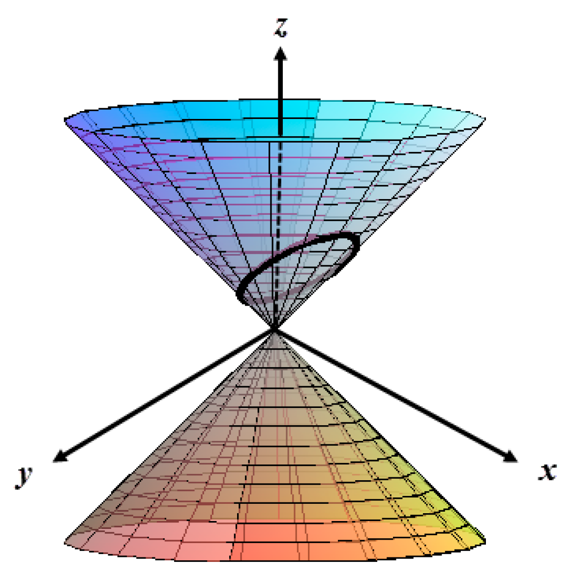
If the dual structure function of $\tilde{\mathit{x}}(s)$ is $\overline{f}\left(s\right)={\displaystyle \frac{2}{\overline{a}}}\tan \left({\displaystyle \frac{\overline{a}s}{2}}\right)$, then the dual curve $\tilde{\mathit{x}}(s)$ can be written as

$$\tilde{\mathit{x}}(s)=\overline{v}\left({\displaystyle \frac{2}{{\overline{a}}^2}}{\sin }^2\left({\displaystyle \frac{\overline{a}s}{2}}\right)-{\displaystyle \frac{1}{2}}{\cos }^2\left({\displaystyle \frac{\overline{a}s}{2}}\right),{\displaystyle \frac{1}{\overline{a}}}\sin \left({\displaystyle \frac{\overline{a}s}{2}}\right),{\displaystyle \frac{2}{{\overline{a}}^2}}{\sin }^2\left({\displaystyle \frac{\overline{a}s}{2}}\right)+{\displaystyle \frac{1}{2}}{\cos }^2\left({\displaystyle \frac{\overline{a}s}{2}}\right)\right).$$

(51)

In this case, the real indicatrix of $\tilde{\mathit{x}}(s)$ is an ellipse (Figure 1).

ii. 

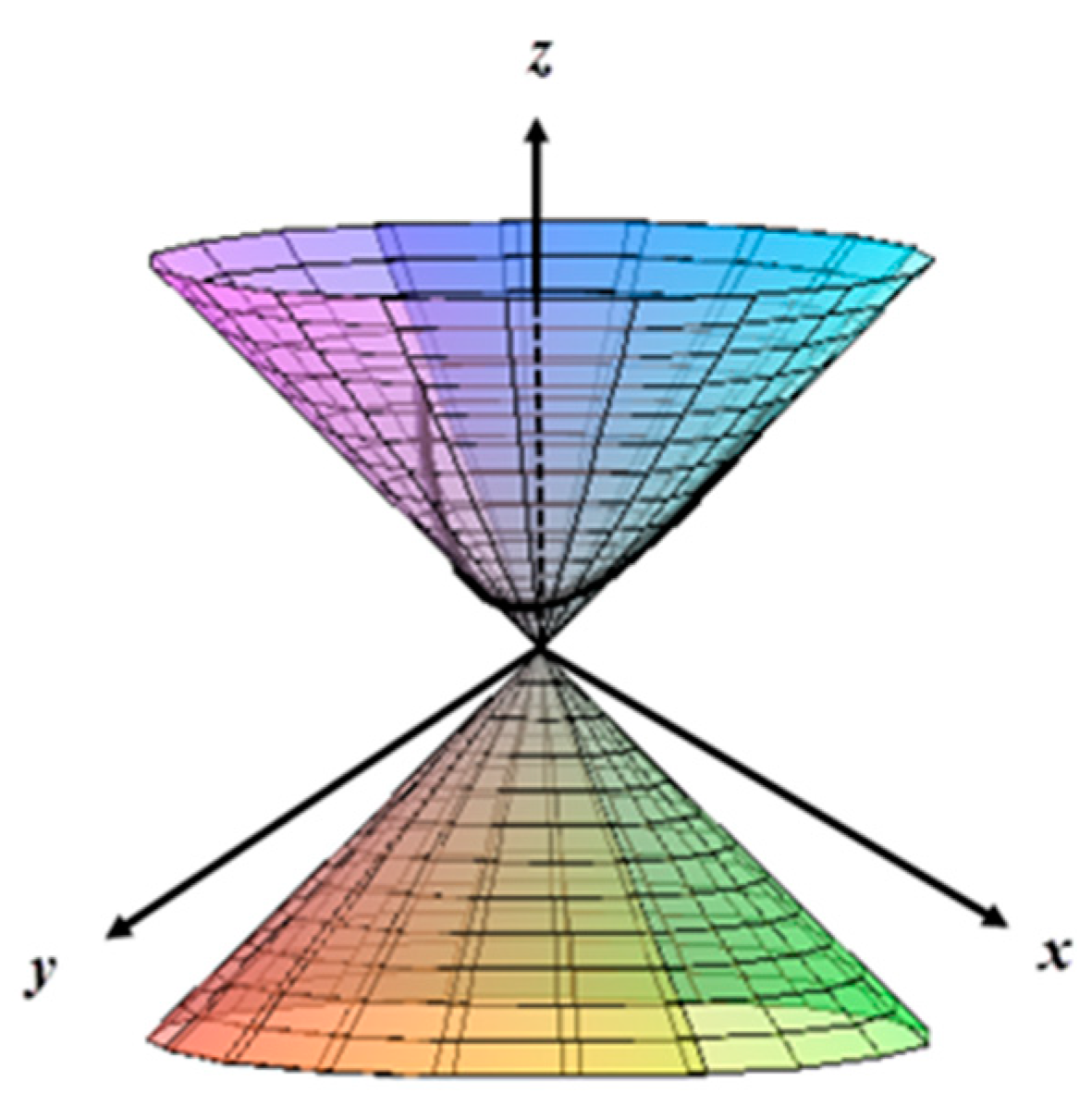
If the dual structure function of $\tilde{\mathit{x}}(s)$ is $\overline{f}\left(s\right)={\displaystyle \frac{\overline{a}}{s}}$, then the dual curve $\tilde{\mathit{x}}(s)$ can be written as

$$\tilde{\mathit{x}}(s)=\overline{v}\left({\displaystyle \frac{\overline{a}}{2}}-{\displaystyle \frac{s^2}{2\overline{a}}},-s,{\displaystyle \frac{\overline{a}}{2}} +{\displaystyle \frac{s^2}{2\overline{a}}}\right).$$

(52)

In this case, the real indicatrix of $\tilde{\mathit{x}}(s)$ is a parabola (Figure 2).

iii. 

If the dual structure function of $\tilde{\mathit{x}}(s)$ is $\overline{f}(s)={\displaystyle \frac{2}{\overline{a}}}\tanh {\displaystyle \frac{\overline{a}}{2}}s$, then the dual curve $\tilde{\mathit{x}}(s)$ can be written as

$$\tilde{\mathit{x}}(s)=\overline{v}\left({\displaystyle \frac{2}{{\overline{a}}^2}}{\sinh }^2\left({\displaystyle \frac{\overline{a}s}{2}}\right)-{\displaystyle \frac{1}{2}}{\cosh }^2\left({\displaystyle \frac{\overline{a}s}{2}}\right),{\displaystyle \frac{1}{\overline{a}}}\sinh \left({\displaystyle \frac{\overline{a}s}{2}}\right),{\displaystyle \frac{2}{{\overline{a}}^2}}{\sinh }^2\left({\displaystyle \frac{\overline{a}s}{2}}\right)+{\displaystyle \frac{1}{2}}{\cosh }^2\left({\displaystyle \frac{\overline{a}s}{2}}\right)\right).$$

(53)

In this case, the real indicatrix of $\tilde{\mathit{x}}(s)$ is a hyperbola (Figure 3).

Definition 4.

Let $\tilde{\mathit{x}}(s)$ be the dual spacelike curve in ${\tilde{\mathit{Q}}}^2$ with parameter $s$ and the dual structure function $\overline{f}\left(s\right)$. If the dual cone curvature $\overline{\kappa }(s)=const.$, then one of the following applies:

i. 

When $-{\overline{a}}^2=\overline{c}$, $a>0$; then, the real indicatrix curve $\mathit{x}(s)$ is an ellipse. In this case, the curve $\tilde{\mathit{x}}(s)$ is called the dual ellipse.

ii. 

When $\overline{c}=0$, the real indicatrix curve $\mathit{x}(s)$ is a parabola. In this case, the curve $\tilde{\mathit{x}}(s)$ is called the dual the parabola.

iii. 

When ${\overline{a}}^2=\overline{c}$, $a>0$; then, the real indicatrix curve $\mathit{x}(s)$ is a hyperbola. In this case, the curve $\tilde{\mathit{x}}(s)$ is called the dual hyperbola.

Example 1.

Let us consider the dual spacelike curve $\tilde{\mathit{x}}(s)=(\cos s,\sin s,1)+\epsilon (-1,0,-\cos s)$, which lies on the dual lightlike cone.

The dual asymptotic frame elements of $\tilde{\mathit{x}}(s)$ are

$$\tilde{\mathit{x}}(s)=(\cos s,\sin s,1)+\epsilon (-1,0,-\cos s),$$

$$\tilde{\alpha }\left(s\right)=(-\sin s,\cos s,0)+\epsilon (0,0,\sin s),$$

$$\tilde{\mathit{y}}(s)={\displaystyle \frac{1}{2}}\left(\cos s,\sin s,-1\right)+{\displaystyle \frac{\epsilon }{2}}\left(1,0,3\cos s\right).$$

The dual cone Frenet formulae for $\tilde{\mathit{x}}(s)$ are given by

$${\tilde{\mathit{x}}}^{\prime }(s)=\left(-\sin s,\cos s,0\right)+\epsilon \left(0,0,\sin s\right),$$

$${\tilde{\alpha }}^{\prime }(s)=\left(-\cos s,-\sin s,0\right)+\epsilon \left(0,0,\cos s\right),$$

$${\tilde{\mathit{y}}}^{\prime }(s)={\displaystyle \frac{1}{2}}\left(-\sin s,\cos s,0\right)+{\displaystyle \frac{\epsilon }{2}}\left(0,0\sin s\right)$$

The structure function is given by

$$\overline{f}={\displaystyle \frac{\cos s+1}{\sin s}}-\epsilon {\displaystyle \frac{\cos s+1}{\sin s}}$$

Dual associated curve of $\tilde{\mathit{x}}(s)$ is denoted by

$$\tilde{\mathit{y}}(s)={\displaystyle \frac{1}{2}}\left(\cos ,\sin s,-1\right)+{\displaystyle \frac{\epsilon }{2}}\left(1,0,3\cos s\right)$$

The dual quasi-Darboux vector for the spacelike curve $\tilde{\mathit{x}}(s)$ is

$$\tilde{\mathit{w}}(s)=\left(0,0,-1\right)+\epsilon \left(1,0,2\cos s\right)$$

Example 2.

Let us consider the dual spacelike curve $\tilde{\mathit{x}}(s)=(-\sin s,\cos s,1)+\epsilon (-\sin s,\cos s,1)$, which lies on the dual lightlike cone.

The vectors of the dual asymptotic frame of $\tilde{\mathit{x}}(s)$ are

$$\tilde{\mathit{x}}(s)=(-\sin s,\cos s,1)+\epsilon (-\sin s,\cos s,1)$$

$$\tilde{\alpha }(s)=(-\cos s,-\sin s,0)$$

$$\tilde{\mathit{y}}(s)={\displaystyle \frac{1}{2}}\left(-\sin s,\cos s,-1\right)+{\displaystyle \frac{\epsilon }{2}}\left(\sin s,-\cos s,1\right)$$

The dual cone Frennet formulae of $\tilde{\mathit{x}}(s)$ are

$${\tilde{\mathit{x}}}^{\prime }(s)=\left(-\cos s,-\sin s,0\right)+\epsilon \left(-\cos s,-\sin s,0\right)$$

$${\tilde{\alpha }}^{\prime }(s)=\left(\sin s,-\cos s,0\right)$$

$${\tilde{\mathit{y}}}^{\prime }(s)={\displaystyle \frac{1}{2}}\left(-\cos s,-\sin s,0\right)+{\displaystyle \frac{\epsilon }{2}}\left(\cos s,\sin s,0\right)$$

The structure function is

$$\overline{f}={\displaystyle \frac{-\sin s+1}{\cos s}}.$$

Dual associated curve of $\tilde{\mathit{x}}(s)$ is

$$\tilde{\mathit{y}}(s)={\displaystyle \frac{1}{2}}\left(-\sin s,\cos s,-1\right)+{\displaystyle \frac{\epsilon }{2}}\left(\sin s,-\cos s,1\right).$$

The quasi-Darboux vector of the spacelike curve $\tilde{\mathit{x}}(s)$ is

$$\tilde{\mathit{w}}(s)=\left(0,0,-1\right)+\epsilon \left({\displaystyle \frac{1}{2}}\sin s,-{\displaystyle \frac{1}{2}}\cos s,{\displaystyle \frac{1}{2}}\right).$$

4. Conclusions

In this study, the mathematical structure of the dual spacelike curves on the dual light cone was examined, and various properties were revealed. Using the dual cone Frenet formulae and the dual cone curvature function, the characteristic properties of the dual spacelike curves were determined, and their structures were related to the dual structure functions. Furthermore, the solutions to the obtained differential equations showed that the real parts of the curves correspond to ellipses, parabolas, and hyperbolas on the light cone, respectively. This finding provides a deeper understanding of the dual structures. Additionally, the curves corresponding to the obtained dual structure functions were defined as the dual ellipse, dual parabola, and dual hyperbola. The results of this study provide a foundation for future research on curves in the dual and dual Lorentzian spaces. In particular, a more detailed investigation of the curves on the dual Lorentzian hyperbolic and Lorentzian spheres could further expand our theoretical understanding in this area. Future studies could deepen the analysis of these results, offering new perspectives on the dual spaces and Lorentzian geometry.