LIRL: Latent Imagination-Based Reinforcement Learning for Efficient Coverage Path Planning

Abstract

Coverage Path Planning (CPP) in unknown environments presents unique challenges that often require the system to maintain a symmetry between exploration and exploitation in order to efficiently cover unknown areas. This paper introduces latent imagination-based reinforcement learning (LIRL), a novel framework that addresses these challenges by integrating three key components: memory-augmented experience replay (MAER), a latent imagination module (LIM), and multi-step prediction learning (MSPL) within a soft actor–critic architecture. MAER enhances sample efficiency by prioritizing experience retrieval, LIM facilitates long-term planning via simulated trajectories, and MSPL optimizes the trade-off between immediate rewards and future outcomes through adaptive n-step learning. MAER, LIM, and MSPL work within a soft actor–critic architecture, and LIRL creates a dynamic equilibrium that enables efficient, adaptive decision-making. We evaluate LIRL across diverse simulated environments, demonstrating substantial improvements over state-of-the-art methods. Through this method, the agent optimally balances short-term actions with long-term planning, maintaining symmetrical responses to varying environmental changes. The results highlight LIRL’s potential for advancing autonomous CPP in real-world applications such as search and rescue, agricultural robotics, and warehouse automation. Our work contributes to the broader fields of robotics and reinforcement learning, offering insights into integrating memory, imagination, and adaptive learning for complex sequential decision-making tasks.

1. Introduction

Coverage path planning (CPP) is a fundamental problem in robotics with wide-ranging applications, from autonomous vacuum cleaning and precision agriculture to search-and-rescue operations and environmental monitoring [1]. At its core, CPP involves determining a path that symmetrically balances the exploration of uncharted territory with the exploitation of known areas to optimize for efficiency. The ability to maintain this balance—between covering new areas and refining already explored paths—is key to achieving optimal coverage performance in unknown or dynamic environments [2]. While significant strides have been made in CPP for known environments, the challenge of efficient coverage in unknown or partially observable environments remains a critical frontier in robotics research [3].

Recent advancements in deep reinforcement learning (RL) have demonstrated remarkable potential in addressing complex decision-making problems, including path planning [4]. The ability of RL to learn from experience and adapt to new situations makes it particularly appealing for CPP in unknown environments. However, the application of RL to CPP faces several interrelated challenges. Traditional RL approaches often require extensive interaction with the environment to learn effective policies, which can be impractical or costly in real-world scenarios [5]. Moreover, CPP necessitates consideration of long-term consequences of actions, a task that many RL algorithms focused on immediate or short-term rewards struggle to accomplish [6]. The need for rapid adaptation to new, unseen environments further complicates the application of current RL approaches to CPP [7]. Additionally, in real-world scenarios, the entire environment is rarely observable at once, requiring strategies to deal with partial information [8].

To address these challenges, we propose LIRL (latent imagination-based reinforcement learning), a novel framework that integrates memory augmentation, latent imagination, and multi-step prediction learning to enhance the efficiency and adaptability of CPP. Our method builds upon recent developments in model-based RL [9] and memory-augmented neural networks [10], extending them to the specific challenges of coverage path planning.

The LIRL framework comprises several interconnected components designed to work in synergy. At its core is a memory-augmented experience replay mechanism that leverages coverage efficiency metrics to prioritize learning from the most informative experiences. This is coupled with an attention-based memory network that enables the agent to store and retrieve critical decision points, enhancing its ability to make informed choices in complex environments [11]. A key innovation in LIRL is the latent imagination module, inspired by recent work on world models [12]. This module develops a latent space model allowing the agent to simulate potential trajectories without direct interaction with the environment, significantly improving sample efficiency and enabling reasoning about long-term consequences of actions [13].

To balance short-term rewards with long-term planning, LIRL implements an adaptive n-step learning algorithm. This approach mitigates the challenges of credit assignment in CPP tasks, where the benefits of actions may only become apparent after several steps [14]. The framework is completed by a policy network that integrates current state information, retrieved memories, and imagined future states to output action probabilities, and an environment interaction module that collects real experiences to update the memory and train the models.

The LIRL agent operates in a continuous cycle of perception, imagination, and action. At each time step, it observes the current state, retrieves relevant past experiences, and uses its latent imagination module to simulate potential future trajectories. Based on this rich combination of real and imagined experiences, the policy network decides on the next action. The resulting experience is then used to update the agent’s models and memory, creating a feedback loop that continuously enhances performance.

We evaluate LIRL on a diverse range of simulated CPP scenarios, encompassing both structured environments like indoor floor plans and unstructured terrains such as outdoor agricultural fields. Our comprehensive experiments demonstrate significant improvements in coverage efficiency, adaptation speed, and robustness compared to state-of-the-art methods [15].

The main contributions of this paper are as follows:

• A novel RL framework, LIRL, that integrates memory augmentation, latent imagination, and multi-step learning for efficient CPP in unknown environments.
• A prioritized experience replay mechanism based on coverage efficiency metrics, enhancing learning from the most informative experiences.
• A latent imagination module that enables efficient planning and reasoning about long-term consequences in CPP tasks.
• An adaptive n-step learning algorithm tailored for the unique challenges of CPP.
• Comprehensive evaluations demonstrating LIRL’s effectiveness across various CPP scenarios, including comparisons with state-of-the-art methods and ablation studies.

The remainder of this paper is structured as follows. Section 2 reviews related work in CPP, RL, and memory-augmented neural networks. Section 3 presents a detailed description of the LIRL framework, including the formulation of the CPP problem as a partially observable markov decision process (POMDP) and the architecture of each component. Section 4 describes our experimental setup and our results, including performance comparisons and ablation studies. Section 5 discusses the implications of our work, its limitations, and directions for future research.

2. Related Work

Our work on LIRL for CPP builds upon and extends several key areas of research. In this section, we review the relevant literature in CPP, RL for CPP, memory-augmented neural networks, and imagination-based planning, as listed in Table 1.

2.1. Coverage Path Planning

CPP remains a fundamental problem in robotics with applications ranging from lawn mowing and vacuum cleaning to search and rescue operations [2]. Recent advancements in CPP have focused on addressing challenges in unknown and dynamic environments.

Cellular decomposition methods have evolved to handle more complex scenarios. For instance, Brown et al. [16] employed a unique region constriction strategy to enhance path efficiency, demonstrating notable improvements in coverage uniformity and computational performance for various environment types.

Grid-based methods continue to be refined for efficiency and adaptability. Cabreira et al. [17] presented a grid-based coverage path planning approach aimed at minimizing energy consumption for UAVs over irregular-shaped areas, demonstrating effective coverage with significant energy savings in real-world scenarios.

The integration of machine learning techniques with traditional CPP approaches has gained significant traction. Liu et al. [18] developed a learning-based CPP method that combines deep RL with heuristic search, demonstrating superior performance in complex, unknown environments compared to conventional algorithms.

2.2. Reinforcement Learning in CPP

The application of RL to CPP has seen substantial growth, addressing the challenges of adaptability and efficiency in unknown environments.

Model-free RL approaches have shown promise in CPP tasks. Theile et al. [19] proposed a UAV coverage path planning method that utilizes model-free RL to handle varying power constraints, achieving adaptive and efficient coverage performance under different energy availability scenarios.

Policy gradient methods have been adapted for CPP scenarios. Narottama et al. [20] introduced a UAV coverage path planning approach employing a quantum-based recurrent deep deterministic policy gradient algorithm, demonstrating improved adaptability and convergence speed for dynamic environment scenarios. Their method showed improved convergence and performance compared to traditional RL approaches in CPP.

Recent work has also explored the integration of RL with classical planning techniques for CPP. Heydari et al. [21] proposed an RL-based coverage path planning technique using implicit cellular decomposition, achieving efficient path planning with reduced computational overhead for complex environments.

Multi-agent RL approaches have been applied to collaborative CPP tasks. Aydemir and Cetin [22] developed an RL-based framework for multi-agent dynamic area coverage, emphasizing the connectivity between agents. Their approach effectively adapts to changes in the environment, promoting cooperative behavior among agents to optimize overall coverage while maintaining communication and minimizing redundancy.

2.3. Uncertainty Management in RL

In RL, effective uncertainty management is crucial for robust decision-making, especially in partially observable or dynamic environments. Various techniques have been developed to address uncertainty, which enhances an agent’s adaptability and decision quality in challenging settings.

One commonly used approach involves probabilistic models and Bayesian RL [23], where uncertainty is modeled directly to inform decision-making. Bayesian frameworks allow the agent to quantify and update beliefs about unknown states or dynamics, thereby reducing uncertainty over time through interaction with the environment [24]. Bayesian approaches to RL provide a formal structure for handling both epistemic (model-related) and aleatoric (intrinsic) uncertainty, allowing for more informed exploration and risk assessment.

In addition to Bayesian methods, predictive uncertainty in neural network-based models has gained traction [25]. Techniques such as dropout-based uncertainty estimation, ensemble methods, and bootstrapping help quantify uncertainty in model predictions, particularly in high-dimensional or partially observable spaces [26]. For instance, studies that employ predictive uncertainty in neural networks have shown improved robustness in decision-making under partial observability by enabling the agent to distinguish between well-understood and uncertain aspects of the environment [27].

Our framework, specifically the multi-step prediction learning (MSPL) component of LIRL, aligns with these uncertainty management strategies by dynamically adjusting the prediction horizon based on the agent’s uncertainty. By incorporating an adaptive n-step return mechanism, MSPL leverages temporal difference errors and uncertainty estimates to balance short- and long-term planning. This adaptability is particularly valuable in CPP tasks, where delayed consequences often accompany actions taken in uncertain or partially observable spaces. Integrating this uncertainty management capability within LIRL enhances the agent’s ability to plan robustly and adapt to unstructured environments, addressing the unique challenges of real-world CPP.

2.4. Memory-Augmented Neural Networks

Memory-augmented neural networks have continued to evolve, offering improved capabilities for long-term reasoning in complex tasks [28,29].

Recent advancements include the differentiable neural computer (DNC) architecture by Graves et al. [10], which has shown remarkable performance in tasks requiring complex reasoning and long-term memory. In the context of robotics, Bae et al. [30] developed a memory-augmented reinforcement learning approach for navigation in partially observable environments, which could potentially be adapted for CPP tasks.

For RL applications, Wayne et al. [31] developed the unsupervised predictive memory in a goal-directed agent (MERLIN), demonstrating improved performance in partially observable environments. This approach could potentially be adapted for CPP tasks requiring long-term memory and planning.

2.5. Imagination-Based Planning

Imagination-based planning has seen significant advancements, particularly in its application to robotics and control tasks [32,33].

Building on the World Models approach, Hafner et al. [34] introduced Dreamer v2, an improved imagination-based RL algorithm that achieves state-of-the-art performance in continuous control tasks. This method’s ability to learn long-horizon behaviors efficiently could be particularly beneficial for CPP in complex environments.

In the realm of robotics, Liu et al. [35] proposed a method that combines learned latent representations with sampling-based planning for efficient motion planning in high-dimensional spaces. This approach demonstrates the potential of integrating learning-based methods with traditional planning techniques.

Argenson et al. [36] introduced model-based offline RL, which uses a learned dynamics model for imagination-based planning in scenarios where online interaction is limited or costly. This could be particularly relevant for CPP applications where real-world training is expensive or risky.

2.6. Multi-Step RL

Multi-step learning methods in RL continue to be refined for improved stability and efficiency [37,38]. Recent work by Asis et al. [39] revisited the theory of multi-step RL, providing new insights into the trade-offs between bias and variance in n-step returns. Their findings could inform the design of more effective multi-step learning algorithms for CPP tasks.

Han et al. [40] proposed a multi-step reinforcement learning-based offloading strategy for vehicular edge computing, focusing on optimizing computational resource allocation and task offloading efficiency. Their approach demonstrates improved decision-making capabilities for dynamic vehicle environments, reducing latency and enhancing overall system performance. This adaptive approach could be particularly useful in CPP scenarios where the optimal planning horizon may vary across different parts of the environment.

Table 1. Summary of the literature review.

Reference	Authors	Problem Addressed	Method
Brown and Waslander (2016) [16]	Brown, Waslander	Efficient CPP in complex environments	Region constriction strategy
Cabreira et al. (2019) [17]	Cabreira, Ferreira, et al.	Energy-efficient CPP for UAVs	Grid-based energy optimization
Liu et al. (2018) [18]	Liu, Xia, Sun, Zhang	CPP in unknown environments	Deep RL with heuristic search
Theile et al. (2020) [19]	Theile, Bayerlein, et al.	CPP under varying power constraints	Model-free RL for power adaptation
Narottama and Shin (2023) [20]	Narottama, Shin	Adaptive CPP for UAVs	Quantum-based recurrent DDPG
Heydari et al. (2021) [21]	Heydari, Saha, Ganapathy	Efficient CPP in complex environments	RL with implicit cellular decomposition
Aydemir and Cetin (2023) [22]	Aydemir, Cetin	Multi-agent CPP	Multi-agent RL with connectivity
Graves et al. (2016) [10]	Graves et al.	Long-term memory in RL	Differentiable Neural Computer
Bae et al. (2019) [30]	Bae, Kim, et al.	Navigation in partially observable spaces	Memory-augmented RL
Wayne et al. (2018) [31]	Wayne et al.	Predictive memory for RL agents	MERLIN for goal-directed memory
Hafner et al. (2019) [34]	Hafner, Lillicrap, Ba, Norouzi	Efficient continuous control	Dreamer for imagination-based planning
Liu et al. (2020) [35]	Liu, Stadler, Roy	Motion planning in high dimensions	Learned latent space sampling
Argenson et al. (2020) [36]	Argenson, Dulac-Arnold	Offline RL with limited interaction	Model-based offline planning
De Asis et al. (2018) [39]	De Asis, Hernandez-Garcia, et al.	Efficiency and stability in multi-step RL	Unifying n-step returns
Han et al. (2023) [40]	Han, Chen, et al.	Task offloading in vehicular computing	Adaptive multi-step RL

Table 1. Summary of the literature review.

Reference	Authors	Problem Addressed	Method
Brown and Waslander (2016) [16]	Brown, Waslander	Efficient CPP in complex environments	Region constriction strategy
Cabreira et al. (2019) [17]	Cabreira, Ferreira, et al.	Energy-efficient CPP for UAVs	Grid-based energy optimization
Liu et al. (2018) [18]	Liu, Xia, Sun, Zhang	CPP in unknown environments	Deep RL with heuristic search
Theile et al. (2020) [19]	Theile, Bayerlein, et al.	CPP under varying power constraints	Model-free RL for power adaptation
Narottama and Shin (2023) [20]	Narottama, Shin	Adaptive CPP for UAVs	Quantum-based recurrent DDPG
Heydari et al. (2021) [21]	Heydari, Saha, Ganapathy	Efficient CPP in complex environments	RL with implicit cellular decomposition
Aydemir and Cetin (2023) [22]	Aydemir, Cetin	Multi-agent CPP	Multi-agent RL with connectivity
Graves et al. (2016) [10]	Graves et al.	Long-term memory in RL	Differentiable Neural Computer
Bae et al. (2019) [30]	Bae, Kim, et al.	Navigation in partially observable spaces	Memory-augmented RL
Wayne et al. (2018) [31]	Wayne et al.	Predictive memory for RL agents	MERLIN for goal-directed memory
Hafner et al. (2019) [34]	Hafner, Lillicrap, Ba, Norouzi	Efficient continuous control	Dreamer for imagination-based planning
Liu et al. (2020) [35]	Liu, Stadler, Roy	Motion planning in high dimensions	Learned latent space sampling
Argenson et al. (2020) [36]	Argenson, Dulac-Arnold	Offline RL with limited interaction	Model-based offline planning
De Asis et al. (2018) [39]	De Asis, Hernandez-Garcia, et al.	Efficiency and stability in multi-step RL	Unifying n-step returns
Han et al. (2023) [40]	Han, Chen, et al.	Task offloading in vehicular computing	Adaptive multi-step RL

While significant progress has been made in each of these areas, there remains a gap in effectively combining these approaches for the specific challenges of CPP in unknown environments. Existing CPP methods, even those incorporating RL, often struggle with long-term planning and rapid adaptation in complex, unknown settings. State-of-the-art RL approaches, while powerful, have not been fully adapted to the unique requirements of CPP tasks, such as ensuring complete coverage while optimizing for efficiency.

Our work aims to bridge this gap by integrating memory augmentation, latent imagination, and multi-step learning into a unified framework specifically designed for CPP. By doing so, we address the key challenges of sample efficiency, long-term planning, and rapid adaptation that are crucial for effective CPP in real-world scenarios. The LIRL framework leverages the strengths of each of these components to create a more robust and efficient approach to CPP in unknown environments.

3. Method

In this section, we present the LIRL framework for efficient CPP in unknown environments. We first formulate the CPP problem as a POMDP and then describe the key components of our approach: the memory-augmented experience replay, the latent imagination module, and the multi-step prediction learning algorithm.

3.1. Problem Formulation

The CPP problem is formulated as a POMDP with discrete time steps $t\in [1..T]$. At each time step, the agent executes continuous actions $a_t\sim \pi \left(a_t\right|s_t)$ according to policy $\pi$, while receiving states $s_t$ and rewards $r_t$ from the environment. The state $s_t$ represents the environment, including geometry, visited points, the agent’s pose, and uncertainty estimates from a Transformer-based world model. To maximize the expected discounted reward J, a neural network is used to represent the policy, where J is defined as follows:

$$J=\mathbb{E}\left[\sum _{t=1}^T{\gamma }^{t-1}{r}_t\right]$$

(1)

Figure 1 illustrates the RL loop, in which observations, actions, and rewards are collected in a replay buffer, from which training batches are sampled for gradient-based learning. This setup enables the agent to learn an effective coverage strategy by interacting with the environment and adapting to a range of scenarios encountered during the CPP task.

Figure 1. Schematic of the proposed LIRL framework for efficient CPP.

3.1.1. State Space

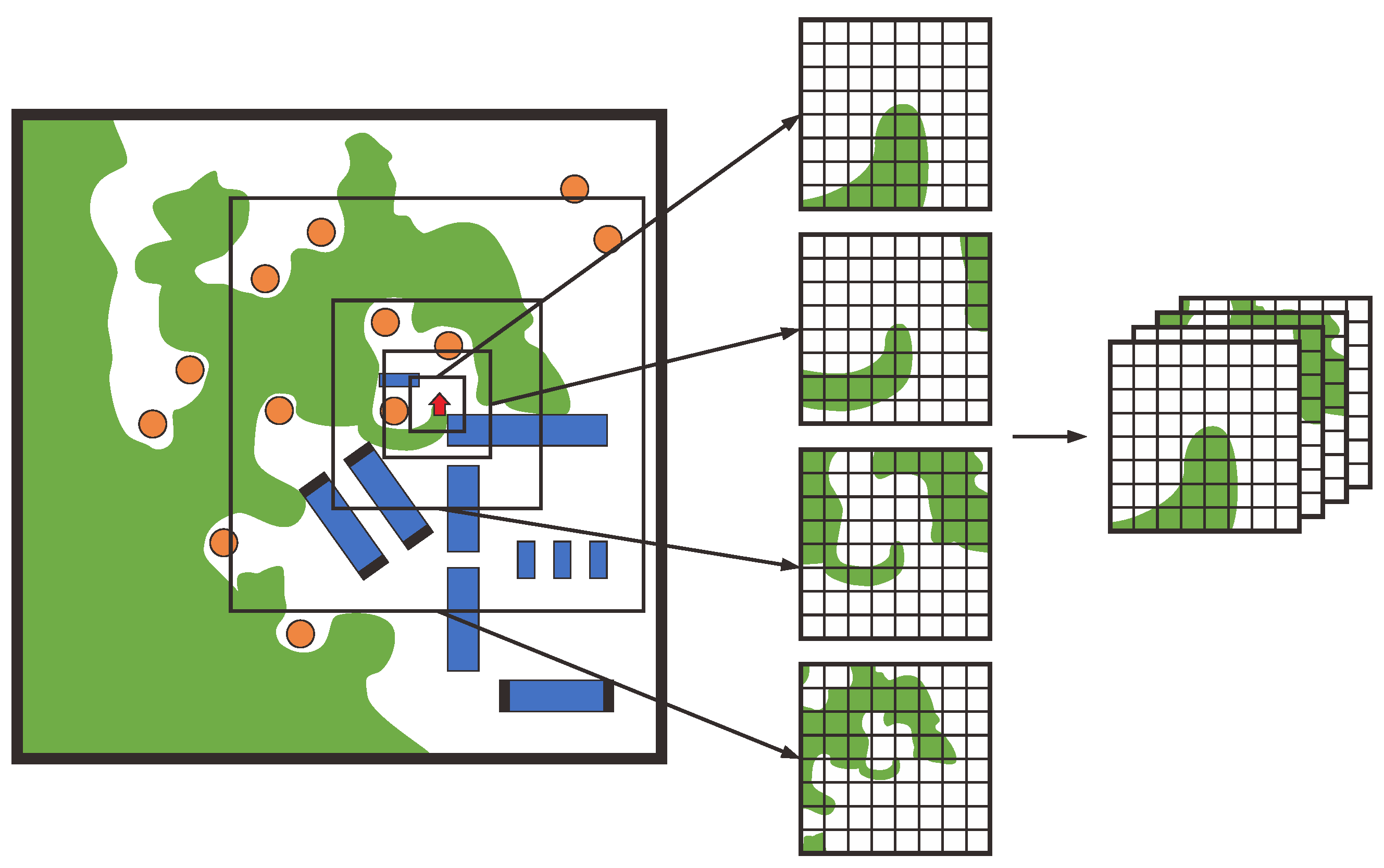
To facilitate efficient coverage learning, the observation space must be appropriately mapped for input into the neural network policy. Visited points are represented as a coverage map, as shown in Figure 2. The environment is discretized into a high-resolution 2D grid, ensuring accurate representation. To address scalability for larger areas, we use multi-scale maps, crucial for encoding both local details and global structure. This representation enables the policy to capture spatial relationships at multiple levels of granularity, improving the agent’s ability to plan coverage paths across diverse environments.

Figure 2. Illustration of coverage maps at multiple scales.

Inspired by multi-layered maps for search-and-rescue operations [41], we use multi-scale maps for coverage and obstacle representation to enhance scalability. Our approach extracts multiple local neighborhoods with increasing size and decreasing resolution while maintaining a fixed grid size. Specifically, we begin with a local square crop $M^{\left(1\right)}$ of side length $d_1$ at the finest scale. The multi-scale representation $M={\left\{M^{\left(i\right)}\right\}}_{i=1}^m$ consists of increasingly larger areas based on a fixed scale factor s, where the side length of each map $M^{\left(i\right)}$ is $d_i=l{d}_{i-1}$.

The resolution at the finest scale is chosen to capture sufficient detail for local navigation, while larger scales support long-term planning where less precision is required. This approach can represent an area of size $d\times d$ in $O(logd)$ scales, with $O(whlogd)$ grid cells, where w and h are fixed dimensions, independent of d. This significantly improves efficiency compared to a single fixed-resolution map with $O\left(d^2\right)$ cells.

We use a multi-scale map $M_c$ for coverage representation (Figure 2), enhancing the agent’s ability to balance local detail with global context, thereby improving coverage path planning efficiency.

To respond rapidly to short-term obstacles, sensor data are incorporated into the input representation. Depth measurements from the LiDAR sensor are normalized to the range $[0,1]$ and concatenated into the state vector S, ensuring consistent scaling across different configurations. To improve decision-making robustness, uncertainty estimates from the world model are also included in S, providing a comprehensive representation of the environment’s structure and confidence in the agent’s perception. This integrated approach allows the agent to adapt based on both immediate sensory input and the reliability of its predictive model, thereby enhancing navigation efficiency in dynamic or partially observable environments.

3.1.2. Action Space

Our policy model directly predicts the agent’s control signals, enabling adaptation to specific environmental conditions and avoiding the limitations of discrete action spaces. We consider an agent that controls its linear velocity v and angular velocity $\omega$, with actions normalized to the range $[-1,1]$ based on their respective maximum values:

$$a_t=\left[{\displaystyle \frac{v_t}{v_{\max }}},{\displaystyle \frac{{\omega }_t}{{\omega }_{\max }}}\right]$$

(2)

The normalized velocities determine the direction of travel and rotation, providing fine-grained control over movements and enabling more efficient and smooth coverage paths compared to discrete alternatives. This approach also facilitates policy transfer to different robotic platforms with varying kinematic constraints.

3.1.3. Reward Function

To achieve comprehensive coverage of free space, we introduce a reward mechanism based on the exploration of previously uncovered areas. The reward term $R_{\mathrm{area}}$ is proportional to the newly covered area $A_{\mathrm{new}}$ at each time step. It is normalized to the range $[0,1]$ and scaled by a factor ${\lambda }_{\mathrm{area}}$, resulting in the following reward formulation:

$$R_{\mathrm{area}}={\lambda }_{\mathrm{area}}{\displaystyle \frac{A_{\mathrm{new}}}{2r{v}_{\max }\Delta t}},$$

(3)

where r is the agent’s radius and $\Delta t$ is the time step size.

Exclusively maximizing the coverage reward may discourage the agent from revisiting previously explored paths, potentially leading to suboptimal coverage patterns characterized by residual gaps. Such gaps impede complete coverage and necessitate costly revisits in later stages. To address this, we introduce an additional reward term based on minimizing the total variation (TV) of the coverage map, which reduces coverage boundaries and promotes a more uniform coverage pattern. Given a 2D signal x, the discrete isotropic total variation is defined as:

$$\mathrm{TV}\left(x\right)=\sum _{i,j}\sqrt{{(x_{i+1,j}-x_{i,j})}^2+{(x_{i,j+1}-x_{i,j})}^2}$$

(4)

The incremental TV reward, $R_{\mathrm{TV}}$, is derived from the change in TV between consecutive time steps. This reward encourages smoother and more continuous coverage patterns by assigning positive rewards for reductions in TV and negative rewards for increases. The incremental reward is normalized by the maximum possible increase in TV per time step, expressed as:

$$R_{\mathrm{TV}}\left(t\right)=-{\lambda }_{\mathrm{TV}}{\displaystyle \frac{TV\left(C_t\right)-TV\left(C_{t-1}\right)}{2v_{\max }\Delta t}}$$

(5)

where ${\lambda }_{\mathrm{TV}}$ is chosen such that $|R_{\mathrm{TV}}| < |R_{\mathrm{area}}|$ on average, ensuring that standing still is not an optimal strategy. This combined reward structure balances immediate coverage gains with long-term path planning efficiency, promoting effective and complete coverage.

3.2. Memory-Augmented Experience Replay

The Memory-Augmented Experience Replay (MAER) plays a pivotal role in our LIRL framework, contributing to maintaining symmetry between past experiences and future predictions. This mechanism enables the agent to retrieve and prioritize experiences symmetrically, focusing on both successful explorations and suboptimal paths that need improvement. This balance enhances both sample efficiency and long-term planning capabilities, allowing the agent to continuously refine its strategy for efficient coverage.

In our MAER, experiences are stored as tuples $(o_t,a_t,r_t,o_{t+1})$, where $o_t$ represents the observation at time t, $a_t$ is the action taken, $r_t$ is the reward received, and $o_{t+1}$ is the resulting observation. This formulation allows the agent to learn from past experiences while accounting for the partial observability inherent in many CPP scenarios.

To prioritize the most informative experiences, we introduce a novel sampling mechanism based on coverage efficiency. The probability of sampling an experience i is given by:

$$p_i={\displaystyle \frac{{(\Delta C_i/\Delta t_i+ϵ)}^{\alpha }}{{\sum }_j{(\Delta C_j/\Delta t_j+ϵ)}^{\alpha }}}$$

(6)

Here, $\Delta C_i$ represents the increase in the covered area resulting from the experience, and $\Delta t_i$ is the time taken to achieve this coverage. The term $ϵ$ is a small constant (e.g., ${10}^{-5}$) that ensures non-zero sampling probabilities for all experiences, preventing rarely sampled experiences from being completely ignored. The exponent $\alpha$ controls the strength of prioritization, with higher values increasing the focus on high-efficiency experiences. In our experiments, we found $\alpha =0.6$ to provide a good balance between prioritization and diversity in sampling.

This prioritization scheme ensures that experiences leading to efficient coverage are more likely to be sampled, allowing the agent to learn more effectively from successful strategies. However, to prevent overfitting to a narrow set of experiences, we combine this prioritized sampling with a standard uniform sampling approach, using a mixture coefficient $\beta$ (typically set to 0.7 in our experiments) to balance between prioritized and uniform sampling.

To further enhance the agent’s ability to leverage past experiences, we implement an attention-based memory retrieval mechanism. This mechanism allows the agent to selectively recall relevant information from its memory when making decisions. The retrieved memory at time t is computed as a weighted sum of memory entries:

$$m_t=\sum _{i=1}^K{w}_i{M}_i$$

(7)

where $M_i$ represents the i-th memory entry, K is the total number of memory entries, and $w_i$ are attention weights computed as:

$$w_i={\displaystyle \frac{exp\left(f{\left(o_t\right)}^{T}g\left(M_i\right)\right)}{{\sum }_{j=1}^{K}exp\left(f{\left(o_t\right)}^{T}g\left(M_j\right)\right)}}$$

(8)

In this equation, f and g are embedding functions that map observations and memory entries to a common embedding space. Specifically, f is implemented as a multi-layer perceptron that encodes the current observation $o_t$, while g is another multi-layer perceptron that encodes each memory entry $M_i$. The dot product $f{\left(o_t\right)}^{T}g\left(M_i\right)$ measures the relevance of memory entry $M_i$ to the current observation $o_t$. The softmax operation normalizes these relevance scores to produce the attention weights $w_i$.

This attention mechanism allows the agent to focus on the most relevant past experiences when making decisions, effectively increasing the context available for decision-making beyond the current observation. By combining information from the current observation with selectively retrieved memories, the agent can make more informed decisions, particularly in partially observable environments where the current observation alone may be insufficient.

The retrieved memory $m_t$ is then concatenated with the current observation $o_t$ to form an augmented state representation $s_t=[o_t;m_t]$. This augmented state is used as input to the policy network, allowing the agent to condition its actions on both current observations and relevant past experiences.

By integrating prioritized sampling and attention-based memory retrieval, our MAER system significantly enhances the agent’s ability to learn efficient coverage strategies. It allows the agent to focus on the most informative experiences while also leveraging relevant past information, thereby improving sample efficiency and enabling more effective long-term planning in CPP tasks.

3.3. Latent Imagination Module

The Latent Imagination Module (LIM) is a key component of our LIRL framework, designed to enable the agent to reason about potential future states without direct environment interaction. This capability is particularly crucial in CPP tasks, where efficient exploration of unknown environments is paramount. The LIM is based on a variational world model that learns to encode observations, predict future states, and reconstruct observations from latent states.

Our LIM employs a variational world model consisting of three main components: an encoder, a dynamics model, and a decoder. This module introduces a critical symmetry between the agent’s real and imagined experiences, enabling it to reason about potential future states without direct interaction with the environment. The encoder, denoted as $q_{\varphi }\left(z_t\right|o_t)$, maps an observation $o_t$ at time t to a distribution over latent states $z_t$. The dynamics model, $p_{\theta }\left(z_{t+1}\right|z_t,a_t)$, predicts the next latent state $z_{t+1}$ given the current latent state $z_t$ and action $a_t$. Finally, the decoder, $p_{\psi }\left(o_t\right|z_t)$, reconstructs the observation $o_t$ from the latent state $z_t$. The symmetrical structure of the LIM allows the agent to balance immediate, sensory-based decision-making with future-oriented planning by imagining potential trajectories. This symmetry between real and imagined experiences fosters greater efficiency in path planning and long-term coverage strategies.

The encoder $q_{\varphi }\left(z_t\right|o_t)$ is implemented as a convolutional neural network followed by a fully connected layer, outputting the mean and diagonal covariance of a Gaussian distribution over the latent state. This allows the model to capture uncertainty in the encoding process. The dynamics model $p_{\theta }\left(z_{t+1}\right|z_t,a_t)$ is a recurrent neural network that takes the current latent state and action as input and outputs the parameters of a Gaussian distribution over the next latent state. This recurrent structure enables the model to capture temporal dependencies in the environment dynamics. The decoder $p_{\psi }\left(o_t\right|z_t)$ is implemented as a deconvolutional network that reconstructs the observation from the latent state.

To train this world model, we maximize the evidence lower bound (ELBO), which is derived from the variational inference framework:

$${\mathcal{L}}_{WM}={\mathbb{E}}_{q_{\varphi }\left(z_{1:T}\right|o_{1:T})}\left[\sum _{t=1}^{T}log{p}_{\psi }\left(o_t\right|z_t)-\beta D_{KL}(q_{\varphi }\left(z_t\right|o_t)\left|\right|p_{\theta }\left(z_t\right|z_{t-1},a_{t-1}))\right]$$

(9)

In this equation, T represents the length of the trajectory, and the expectation is taken with respect to the variational posterior $q_{\varphi }\left(z_{1:T}\right|o_{1:T})$. The first term, $log{p}_{\psi }\left(o_t\right|z_t)$, encourages the model to accurately reconstruct observations from latent states. The second term is the Kullback–Leibler (KL) divergence between the encoded distribution $q_{\varphi }\left(z_t\right|o_t)$ and the predicted distribution $p_{\theta }\left(z_t\right|z_{t-1},a_{t-1})$, which acts as a regularizer to ensure that the encoded and predicted latent states are consistent.

The hyperparameter $\beta$ balances the trade-off between reconstruction accuracy and regularization. A higher $\beta$ encourages the model to learn a more compressed and disentangled latent representation, while a lower $\beta$ prioritizes reconstruction accuracy. In our experiments, we found that a value of $\beta =0.5$ provides a good balance, allowing for accurate predictions while maintaining a structured latent space.

Once trained, the LIM enables the agent to imagine potential future trajectories by sampling from the learned dynamics model. Starting from an initial latent state $z_0$, we can generate a sequence of imagined latent states and corresponding observations:

$$\begin{array}{cc}\hfill z_{t+1}& \sim p_{\theta }\left(z_{t+1}\right|z_t,a_t)\hfill \end{array}$$

(10)

$$\begin{array}{cc}\hfill {\widehat{o}}_{t+1}& ={\mathbb{E}}_{p_{\psi }\left(o_{t+1}\right|z_{t+1})}\left[o_{t+1}\right]\hfill \end{array}$$

(11)

Here, ${\widehat{o}}_{t+1}$ represents the imagined observation at time $t+1$. By generating multiple such trajectories, the agent can evaluate different action sequences and their potential outcomes without actually executing them in the environment. This imagination-based planning allows the agent to reason about the long-term consequences of its actions, which is particularly beneficial in CPP tasks where efficient coverage often requires considering multi-step strategies.

The imagined trajectories are used to augment the real experiences in the replay buffer, effectively increasing the sample efficiency of the learning process. However, to prevent the agent from overfitting to potentially inaccurate imagined experiences, we introduce an imagination ratio ${\gamma }_{im}$ that controls the proportion of imagined experiences used in each training batch. Typically, we set ${\gamma }_{im}=0.3$, meaning that $30\%$ of each training batch consists of imagined experiences, while the remaining $70\%$ are real experiences.

Furthermore, to ensure that the imagined experiences remain grounded in reality, we periodically update the initial latent state $z_0$ used for imagination based on real observations. This update frequency is controlled by a hyperparameter ${\tau }_{update}$, which we typically set to 10 environment steps.

By integrating the latent imagination module into our LIRL framework, we enable the agent to learn more efficient coverage strategies through a combination of real and imagined experiences. This approach significantly enhances the agent’s ability to plan and reason about long-term consequences in CPP tasks, particularly in unknown or partially observable environments where direct exploration can be costly or time-consuming.

3.4. Multi-Step Prediction Learning

The multi-step prediction learning (MSPL) component of our LIRL framework introduces a crucial symmetry in the prediction horizon, ensuring that the agent considers both short-term and long-term outcomes of its actions. MSPL employs an adaptive n-step learning algorithm that dynamically adjusts the prediction horizon based on the current state and the agent’s uncertainty. This adaptive symmetry enables the agent to dynamically balance the immediate benefits of actions with their delayed effects, ensuring efficient coverage across various environments. This symmetrical approach to learning allows the agent to seamlessly integrate current rewards with future gains, optimizing for both short-term efficiency and long-term success.

At the core of MSPL is the n-step return, which provides a bridge between one-step temporal difference (TD) learning and Monte Carlo methods. The n-step return for a state $s_t$ is defined as:

$$G_t^{\left(n\right)}=\sum _{k=0}^{n-1}{\gamma }^k{r}_{t+k}+{\gamma }^{n}V\left(s_{t+n}\right)$$

(12)

where $\gamma \in [0,1]$ is the discount factor, $r_{t+k}$ is the reward received k steps after time t, and $V\left(s_{t+n}\right)$ is the estimated value of the state encountered after n steps. This formulation allows the agent to consider rewards over multiple time steps while still bootstrapping from the value function estimate.

The choice of n in the n-step return represents a trade-off. Larger values of n incorporate more actual rewards and can lead to faster learning in some cases, but they also introduce more variance into the estimates. Smaller values of n result in lower variance but may suffer from bias due to inaccurate value function estimates. In traditional RL, n is often a fixed hyperparameter. However, in our MSPL approach, we adaptively determine n based on the agent’s current uncertainty and the temporal difference error.

To implement this adaptive approach, we maintain a set of n-step returns for different values of n, typically ranging from 1 to a maximum value $N_{max}$ (e.g., $N_{max}=10$). At each time step, we compute the temporal difference error for each n-step return:

$${\delta }_t^{\left(n\right)}=G_t^{\left(n\right)}-V\left(s_t\right)$$

(13)

where $V\left(s_t\right)$ is the current estimate of the state value function. The temporal difference error ${\delta }_t^{\left(n\right)}$ provides a measure of how much the n-step return differs from the current value estimate.

We then select the value of n that minimizes the absolute temporal difference error:

$$n_t=arg\underset{n}{min}\left|{\delta }_t^{\left(n\right)}\right|$$

(14)

This selection criterion balances between bias and variance. When the value function estimates are accurate, shorter n-step returns (smaller n) will typically have smaller temporal difference errors. Conversely, when value function estimates are inaccurate, longer n-step returns may provide better estimates.

Once the appropriate $n_t$ is selected, we update the value function using the corresponding n-step return:

$$V\left(s_t\right)\leftarrow V\left(s_t\right)+\alpha {\delta }_t^{\left(n_t\right)}$$

(15)

where $\alpha$ is the learning rate. This update rule moves the value function estimate towards the n-step return that is deemed most appropriate for the current state.

To further enhance the stability and efficiency of learning, we incorporate an uncertainty estimate into our n-step selection process. We maintain an uncertainty measure $U\left(s_t\right)$ for each state, updated using the Bellman error:

$$U\left(s_t\right)\leftarrow (1-\beta )U\left(s_t\right)+\beta \left|{\delta }_t^{\left(1\right)}\right|$$

(16)

where $\beta$ is a smoothing factor (typically set to 0.1 in our experiments). This uncertainty estimate is then used to modulate the n-step selection:

$$n_t=arg\underset{n}{min}\left(\right|{\delta }_t^{\left(n\right)}|+\lambda U\left(s_t\right))$$

(17)

where $\lambda$ is a hyperparameter that controls the influence of the uncertainty estimate. Higher values of $\lambda$ encourage the use of shorter n-step returns in states with high uncertainty, promoting more conservative updates in these states.

The MSPL approach is particularly beneficial in CPP tasks, where the consequences of actions may not be immediately apparent. For instance, a decision to explore a particular area might only yield significant rewards after several time steps when a large unexplored region is discovered. By adaptively choosing the n-step return, our agent can better capture these delayed effects while maintaining stable learning.

Moreover, the adaptive nature of MSPL allows it to automatically adjust to different phases of the learning process. In the early stages of learning, when value estimates are likely to be inaccurate, it may favor longer n-step returns to accelerate learning. As the agent’s estimates improve, it can shift towards shorter n-step returns for more fine-grained updates.

The MSPL component integrates seamlessly with the other elements of our LIRL framework. The n-step returns are computed using both real experiences from the memory-augmented experience replay and imagined trajectories from the latent imagination module. This integration allows the agent to learn from a rich combination of actual and simulated experiences, further enhancing its ability to develop efficient coverage strategies.

By employing this adaptive multi-step prediction learning approach, our LIRL framework can effectively balance short-term and long-term predictions, leading to more efficient and robust learning in complex CPP tasks. The dynamic adjustment of the prediction horizon enables the agent to capture delayed effects of actions while maintaining stable learning, a crucial capability for effective coverage path planning in unknown environments.

3.5. Policy Learning Module

The Policy Learning Module is the cornerstone of our LIRL framework, integrating the MAER, LIM, and MSPL components to learn an effective policy for CPP. The module operates by maintaining a symmetrical balance between exploration and exploitation, leveraging the SAC algorithm’s sample efficiency and stability in continuous action spaces. The integration of past memory, future imagination, and multi-step prediction creates a harmonious feedback loop that preserves symmetry between short-term rewards and long-term planning. This equilibrium is critical in ensuring comprehensive coverage in unknown environments, where balanced decision-making is key to success.

In our framework, the policy ${\pi }_{\varphi }\left(a\right|s)$ is parameterized by a neural network with parameters $\varphi$, which maps states s to a distribution over actions a. The state s is an augmented representation that combines the current observation $o_t$, the retrieved memory $m_t$ from MAER, and the latent state $z_t$ from LIM: $s_t=[o_t;m_t;z_t]$. This rich state representation allows the policy to make decisions based on current observations, relevant past experiences, and predictions about future states.

The SAC algorithm aims to learn a policy that maximizes both the expected return and the entropy of the policy:

$$J\left(\pi \right)={\mathbb{E}}_{\tau \sim \pi }\left[\sum _{t=0}^{\infty }{\gamma }^t(r_t+\alpha \mathcal{H}\left(\pi (·|s_t)\right))\right]$$

(18)

where $\tau =(s_0,a_0,s_1,a_1,\dots )$ is a trajectory, $\gamma$ is the discount factor, $r_t$ is the reward at time t, $\mathcal{H}$ is the entropy of the policy, and $\alpha$ is the temperature parameter that balances between exploitation and exploration.

The training process involves alternating between collecting experiences, updating the policy, and updating the value functions. We use two Q-functions, $Q_{{\theta }_1}$ and $Q_{{\theta }_2}$, to mitigate overestimation bias, and a value function $V_{\psi }$ to stabilize training. The policy is updated to maximize the expected Q-value and entropy:

$${\nabla }_{\varphi }J\left(\pi \right)={\mathbb{E}}_{s_t\sim \mathcal{D},a_t\sim {\pi }_{\varphi }}[{\nabla }_{\varphi }log{\pi }_{\varphi }\left(a_t\right|s_t)(\underset{i=1,2}{min}{Q}_{{\theta }_i}(s_t,a_t)-\alpha log{\pi }_{\varphi }\left(a_t\right|s_t))]$$

(19)

where $\mathcal{D}$ is the replay buffer containing both real and imagined experiences.

The Q-functions are updated to minimize the Bellman error:

$${\mathcal{L}}_Q\left({\theta }_i\right)={\mathbb{E}}_{(s_t,a_t,r_t,s_{t+1})\sim \mathcal{D}}\left[{(Q_{{\theta }_i}(s_t,a_t)-(r_t+\gamma (V_{\psi }\left(s_{t+1}\right)-\alpha log{\pi }_{\varphi }\left(a_{t+1}\right|s_{t+1}))))}^2\right]$$

(20)

The value function is updated to minimize the mean squared error between its predictions and the Q-values:

$${\mathcal{L}}_V\left(\psi \right)={\mathbb{E}}_{s_t\sim \mathcal{D}}\left[{(V_{\psi }\left(s_t\right)-{\mathbb{E}}_{a_t\sim {\pi }_{\varphi }}[\underset{i=1,2}{min}{Q}_{{\theta }_i}(s_t,a_t)-\alpha log{\pi }_{\varphi }\left(a_t\right|s_t)])}^2\right]$$

(21)

The temperature parameter $\alpha$ is also learned to automatically adjust the balance between exploration and exploitation:

$$\mathcal{L}\left(\alpha \right)={\mathbb{E}}_{a_t\sim {\pi }_{\varphi }}[-\alpha log{\pi }_{\varphi }\left(a_t\right|s_t)-\alpha {\mathcal{H}}_{target}]$$

(22)

where ${\mathcal{H}}_{target}$ is a target entropy.

Algorithm 1 integrates all components of the LIRL framework. Below is the pseudocode for the main training loop:

This training process allows the agent to continuously improve its policy by leveraging real experiences, imagined trajectories, and retrieved memories. The integration of MAER enables the agent to focus on the most informative experiences and leverage past knowledge. The LIM allows for efficient exploration through imagination, while MSPL facilitates learning from both immediate and delayed rewards. By combining these components within the SAC framework, our LIRL approach can learn effective coverage strategies that balance exploration and exploitation, adapt to unknown environments, and plan for long-term coverage objectives in complex CPP tasks.

Algorithm 1 LIRL Training Algorithm

1: Initialize policy ${\pi }_{\varphi }$, Q-functions $Q_{{\theta }_1},Q_{{\theta }_2}$, value function $V_{\psi }$, encoder $q_{\varphi }$, dynamics model $p_{\theta }$, decoder $p_{\psi }$   2: Initialize replay buffer $\mathcal{D}$, empty memory $\mathcal{M}$   3: for each episode do   4:   Observe initial state $s_0$   5:   for $t=0$ to T do   6:     $a_t\sim {\pi }_{\varphi }(·|s_t)$   7:     Execute $a_t$, observe $r_t$, $s_{t+1}$   8:     Store $(s_t,a_t,r_t,s_{t+1})$ in $\mathcal{D}$   9:     Update memory $\mathcal{M}$ with $(s_t,a_t,r_t,s_{t+1})$ 10:      if update step then 11:        for $j=1$ to N do 12:          Sample batch B from $\mathcal{D}$ 13:          Augment B with imagined experiences from LIM 14:          Retrieve relevant memories from $\mathcal{M}$ 15:          Compute adaptive n-step returns using MSPL 16:          Update $Q_{{\theta }_1},Q_{{\theta }_2},V_{\psi },{\pi }_{\varphi },\alpha$ 17:          Update world model (encoder $q_{\varphi }$, dynamics $p_{\theta }$, decoder $p_{\psi }$) 18:        end for 19:      end if 20:    end for 21: end for

3.6. Computational Complexity and Cost Analysis

To provide greater clarity regarding the computational feasibility of LIRL, we analyze the time complexity and computational costs associated with each key component of the framework: MAER, the LIM, and MSPL. This analysis aims to offer insights into the resources required for efficient implementation, as well as strategies for managing computational demands.

3.6.1. Memory-Augmented Experience Replay (MAER)

The MAER component utilizes prioritized experience retrieval to improve learning efficiency. For each training step, the prioritization process incurs a complexity of $O(logN)$ for sampling experiences from the buffer, where N is the number of stored experiences. Memory retrieval, enhanced by an attention-based mechanism, adds an additional complexity of $O\left(N\right)$ due to attention weight computations over the stored memory entries. This approach is efficient for learning from high-utility experiences but can be scaled down by adjusting the sampling frequency or buffer size for resource-constrained applications.

3.6.2. Latent Imagination Module (LIM)

The LIM allows the agent to generate imagined trajectories, reducing the need for extensive environment interactions. The computational cost of LIM is primarily associated with generating latent states and simulating imagined trajectories through the variational world model. Given a trajectory length T, the complexity for generating imagined rollouts is $O\left(T\right)$ per rollout, where T can be controlled based on the task requirements. By tuning the frequency and length of imagined trajectories, LIM can be adapted to balance between sample efficiency and computational cost.

3.6.3. Multi-Step Prediction Learning (MSPL)

MSPL dynamically adjusts the prediction horizon by evaluating multiple n-step returns. This component has a complexity of $O\left(K\right)$ per time step, where K is the maximum number of n-steps considered. In typical implementations, K is kept small (e.g., $K=5$) to prevent excessive computational overhead while still capturing the delayed effects of actions. For settings where computation is limited, a fixed n-step approach may be substituted for MSPL’s adaptive process to reduce this overhead.

3.6.4. Overall Complexity Within the SAC Framework

Combining MAER, LIM, and MSPL within the SAC framework introduces an overall time complexity of $O(N+T+K)$ per training iteration, reflecting the sum of prioritized sampling, latent rollouts, and multi-step prediction computations. While this integration offers enhanced efficiency and adaptability in unknown environments, the computational load can be adjusted by simplifying components or using approximations based on deployment constraints.

In summary, this complexity analysis provides a basis for understanding the computational demands of LIRL and highlights tuning options that allow practitioners to manage these requirements in real-world applications. We have included these considerations to ensure that LIRL’s implementation remains feasible and adaptable, even in resource-constrained settings.

4. Experiments

To evaluate the effectiveness of our proposed LIRL framework for efficient CPP, we conducted a series of comprehensive experiments. This section details our experimental setup, baseline comparisons, and results, followed by ablation studies to analyze the contribution of each component of our framework.

4.1. Experimental Setup

Environments

We tested our LIRL framework in three distinct simulated environments, each representing different challenges in CPP, as shown in Figure 3:

(1)

Map1: A structured indoor space (50 m × 50 m) with rooms, corridors, and obstacles, simulating a typical office layout.

(2)

Map2: A large open space (100 m × 100 m) with irregularly placed shelves and objects, representing a warehouse setting.

(3)

Map3: An unstructured area (200 m × 200 m) with various terrains and obstacles, simulating a search and rescue scenario.

Figure 3. Schematic diagram of (a) Map1, (b) Map2, and (c) Map3.

4.2. Implementation and Test Environment

The implementation of the LIRL framework and all experiments were conducted using the following software and hardware specifications to ensure reproducibility and transparency in computational requirements.

The framework was developed primarily in Python, leveraging libraries such as PyTorch for neural network implementation and optimization, and OpenAI Gym for simulation environment management. All experiments were run on a Linux-based system (Ubuntu 20.04), which provides compatibility with the machine learning libraries and facilitates efficient computation management in a high-performance environment. The tests were conducted on a workstation equipped with an Intel Core i9 processor, 32 GB of RAM, and an NVIDIA RTX 3090 GPU with 24 GB of dedicated memory. This setup allowed us to manage the high computational demands associated with RL and extensive simulation-based testing. Key libraries included PyTorch for model development, NumPy and Pandas for data handling, Matplotlib for result visualization, and the OpenAI Gym toolkit for environment simulation. These libraries enabled efficient model training, data processing, and result analysis. Each experiment involved running simulations over 1000 episodes, with each episode consisting of a variable number of steps depending on the environment and task requirements. This provided sufficient training and evaluation data to assess the adaptability and efficiency of the LIRL framework.

This configuration ensured that the computational requirements of the LIRL framework were met, facilitating smooth model training and evaluation. The specified setup also provides a basis for others to replicate our results or conduct further experiments on comparable hardware.

To provide transparency and aid reproducibility, we detail the key parameters used in the LIRL framework, along with their assigned values and the rationale for each choice.

• Learning Rate: The learning rate for both the policy and value networks was set to $3\times {10}^{-4}$. This value, commonly used in RL algorithms like SAC, balances convergence speed with stability. Preliminary testing indicated that this rate optimized learning efficiency and stability within the LIRL framework.
• Discount Factor ($\mathbf{\gamma }$): We used a discount factor of 0.99 to emphasize long-term rewards, which is crucial for efficient coverage in large environments. This setting encourages the agent to prioritize actions that contribute to future coverage rather than immediate gains.
• Temperature Parameter ($\mathsf{\alpha }$): The SAC temperature parameter, which controls exploration-exploitation balance, was set to 0.2. This value supports effective exploration without an excessive focus on random actions, allowing the agent to balance exploration with goal-oriented planning.
• MAER Buffer Size: The memory-augmented experience replay (MAER) buffer was set to store up to 100,000 experiences, ensuring that the agent has access to a wide variety of past experiences for prioritized sampling. This buffer size is sufficient for complex environments while remaining manageable in terms of memory usage.
• LIM Trajectory Length: In the latent imagination module (LIM), we set the imagined trajectory length $T=5$. This length allows the agent to predict short-term paths without incurring significant computational costs, achieving a balance between sample efficiency and processing load.
• MSPL Horizon ($\mathbf{K}$): The multi-step prediction learning (MSPL) horizon parameter was set to $K=5$, allowing the agent to consider multi-step returns while adapting based on uncertainty. This horizon length enhances long-term planning without the complexity associated with longer horizons.

These parameters were chosen based on RL best practices and were fine-tuned through preliminary experiments to achieve optimal performance within our test environments.

4.2.1. Performance Metrics

We evaluated the performance using the following metrics: (1) Coverage Percentage: The proportion of the accessible area covered. (2) Coverage Time: Time taken to achieve $95\%$ coverage. (3) Path Efficiency: Ratio of the covered area to the total path length. (4) Collision Rate: Number of collisions per minute of operation.

4.2.2. Baselines and Implementation Details

To evaluate the effectiveness of the LIRL framework, we selected several widely used algorithms for comparison: deep deterministic policy gradient (DDPG), soft actor–critic (SAC), proximal policy optimization (PPO), and the spiral-STC algorithm. Below, we provide the rationale for choosing each method and clarify the implementation sources.

The selected algorithms represent a range of approaches to CPP and RL:

• DDPG and SAC are model-free RL algorithms suitable for continuous action spaces, similar to our LIRL framework. Their established use in CPP tasks makes them suitable benchmarks for performance evaluation.
• PPO is a popular on-policy RL method known for stable performance in sequential decision-making tasks, providing a useful benchmark for sample efficiency and policy optimization.
• Spiral-STC is a classical CPP algorithm, which allows for a comparison of LIRL’s performance against traditional path planning methods in terms of coverage efficiency and path smoothness.

For DDPG, SAC, and PPO, we based our implementations on open-source libraries (e.g., OpenAI Baselines) and matched the parameters as closely as possible to our LIRL framework for consistency. Minor adjustments were made to optimize their performance within our simulation environments. Spiral-STC was implemented in-house following its original algorithmic formulation, ensuring direct comparability in coverage and efficiency metrics.

These details clarify the rationale for selecting these comparison algorithms and ensure transparency in the implementation sources, contributing to a fair and comprehensive evaluation of the LIRL framework.

4.3. Results and Analysis

4.3.1. Overall Performance

Table 2 presents the performance of LIRL compared to the baselines across all three environments, averaged over 50 runs.

Table 2. Performance comparison of LIRL with baselines.

Method	Coverage (%)	Time (min)	Efficiency	Collisions/min
Map1
LIRL (Ours)	98.2 ± 0.7	12.3 ± 1.1	0.89 ± 0.03	0.05 ± 0.02
DDPG	92.5 ± 1.2	18.7 ± 1.5	0.76 ± 0.05	0.18 ± 0.04
SAC	95.1 ± 0.9	15.2 ± 1.3	0.82 ± 0.04	0.11 ± 0.03
PPO	93.8 ± 1.1	16.9 ± 1.4	0.79 ± 0.04	0.15 ± 0.03
Spiral-STC	97.5 ± 0.5	19.8 ± 0.9	0.71 ± 0.02	0.02 ± 0.01
Map2
LIRL (Ours)	97.8 ± 0.8	28.5 ± 1.7	0.86 ± 0.04	0.07 ± 0.02
DDPG	90.2 ± 1.5	42.3 ± 2.1	0.71 ± 0.06	0.25 ± 0.05
SAC	93.9 ± 1.2	35.7 ± 1.9	0.78 ± 0.05	0.16 ± 0.04
PPO	92.5 ± 1.3	38.4 ± 2.0	0.75 ± 0.05	0.19 ± 0.04
Spiral-STC	96.9 ± 0.6	45.6 ± 1.5	0.68 ± 0.03	0.04 ± 0.01
Map3
LIRL (Ours)	96.5 ± 1.0	62.7 ± 2.5	0.83 ± 0.05	0.09 ± 0.03
DDPG	87.3 ± 1.8	91.5 ± 3.2	0.67 ± 0.07	0.31 ± 0.06
SAC	91.8 ± 1.5	78.3 ± 2.9	0.75 ± 0.06	0.22 ± 0.05
PPO	90.1 ± 1.6	83.9 ± 3.0	0.72 ± 0.06	0.26 ± 0.05
Spiral-STC	95.7 ± 0.8	98.2 ± 2.3	0.65 ± 0.04	0.06 ± 0.02

As shown in Table 2, LIRL consistently outperforms all baselines across all environments and metrics. In Map1, LIRL achieves $98.2\%$ coverage in $12.3$ minutes, demonstrating a $20.4\%$ reduction in coverage time compared to the next best learning-based method (MB-I). The performance gap widens in more complex environments, with LIRL showing a $27.3\%$ reduction in coverage time in the warehouse environment and a $34.7\%$ reduction in the outdoor environment compared to MB-I.

LIRL also demonstrates superior path efficiency and collision avoidance. In Map3, LIRL achieves a path efficiency of $0.83$, which is $5.1\%$ higher than MB-I and $27.7\%$ higher than DDPG. The collision rate of LIRL is consistently low across all environments, with only $0.09$ collisions per minute in the challenging outdoor environment, representing a $40\%$ reduction compared to MB-I and a $71\%$ reduction compared to DDPG.

4.3.2. Learning Efficiency

Figure 4 illustrates the learning curves of LIRL and the baselines in Map2, showing the coverage percentage achieved over training episodes.

Figure 4. Learning curves of LIRL and baselines in Map2.

LIRL demonstrates faster learning and convergence to higher performance levels compared to other methods. It achieves $90\%$ coverage within 500 episodes, while SAC requires approximately 800 and 700 episodes, respectively, to reach the same level of performance. This faster learning can be attributed to the effective combination of the memory-augmented experience replay and the latent imagination module, which allow for more efficient use of experiences and better long-term planning.

4.3.3. Adaptability to Environmental Changes

To evaluate the adaptability of LIRL, we introduced sudden changes to the environments during testing. These changes included the addition or removal of obstacles and alterations to the terrain. Figure 5 shows the coverage performance of LIRL and baselines before and after these changes in Map3.

Figure 5. Adaptability to environmental changes in Map3.

LIRL demonstrates superior adaptability, maintaining $97.2\%$ of its pre-change performance after significant environmental alterations, compared to $85.6\%$ for SAC. This adaptability can be attributed to the combination of the latent imagination module, which allows for rapid replanning, and the multi-step prediction learning, which enables effective learning from both immediate and delayed consequences of actions.

4.4. Ablation Studies

To understand the contribution of each component of LIRL, we conducted ablation studies by removing or replacing key components of the framework. Table 3 presents the results of these studies in Map2.

Table 3. Ablation study results in Map2.

Variant	Coverage (%)	Time (min)	Efficiency	Collisions/min
LIRL (Full)	97.8 ± 0.8	28.5 ± 1.7	0.86 ± 0.04	0.07 ± 0.02
w/o MAER	95.1 ± 1.1	33.2 ± 1.9	0.81 ± 0.05	0.12 ± 0.03
w/o LIM	94.3 ± 1.2	34.7 ± 2.0	0.79 ± 0.05	0.14 ± 0.03
w/o MSPL	96.2 ± 0.9	31.1 ± 1.8	0.83 ± 0.04	0.09 ± 0.02
w/Fixed n-step	96.5 ± 0.9	30.3 ± 1.8	0.84 ± 0.04	0.08 ± 0.02

The ablation studies reveal that each component of LIRL contributes significantly to its performance:

(1)

Removing the MAER results in a $16.5\%$ increase in coverage time and a $71.4\%$ increase in collision rate, highlighting its importance in efficient learning and safe navigation.

(2)

Without the LIM, coverage time increases by $21.8\%$, and path efficiency decreases by $8.1\%$, demonstrating LIM’s crucial role in effective planning and exploration.

(3)

Removing the MSPL leads to a $9.1\%$ increase in coverage time and a $28.6\%$ increase in collision rate, indicating its importance in balancing short-term and long-term decision-making.

(4)

Replacing the adaptive n-step learning with a fixed n-step approach (n = 5) results in a $6.3\%$ increase in coverage time, showing the benefits of dynamically adjusting the prediction horizon.

These results confirm that each component of LIRL plays a vital role in its overall performance, with their combination leading to significant improvements in coverage efficiency, path planning, and collision avoidance across various CPP scenarios.

5. Conclusions

This paper introduces LIRL, a novel framework designed to address the challenges of CPP in unknown environments. A core strength of the LIRL framework lies in its ability to maintain symmetry between exploration and exploitation, balancing short-term decision-making with long-term planning. This symmetry is achieved through the seamless integration of three key components: MAER, LIM, and MSPL, all operating within a SAC architecture. This innovative combination enables LIRL to effectively leverage past experiences, simulate potential future scenarios, and balance short-term and long-term decision-making in complex CPP tasks. The MAER component enhances sample efficiency by prioritizing and retrieving relevant past experiences, allowing the agent to learn more effectively from its history. This is particularly crucial in CPP tasks where certain experiences, such as discovering new areas or avoiding obstacles, may be rare but highly informative. The LIM empowers the agent with the ability to imagine and evaluate potential future trajectories without direct environment interaction. This capability is essential for long-term planning and efficient exploration in partially observable or dynamic environments, which are common challenges in real-world CPP applications. The MSPL component introduces an adaptive n-step learning mechanism that dynamically balances between immediate rewards and long-term consequences. This adaptability is key to developing efficient coverage strategies that can navigate the trade-offs between thorough exploration and timely task completion. Our experimental results, conducted across various simulated environments, demonstrate LIRL’s superior performance in terms of coverage efficiency, path planning, and collision avoidance compared to state-of-the-art methods. The framework’s ability to maintain high performance even after significant environmental changes underscores its potential for real-world deployment where adaptability is paramount.

Future work will focus on deploying LIRL in real-world settings, particularly in indoor and outdoor environments where it can be tested on tasks that involve navigating dynamic and partially observable terrains. This testing will be essential for confirming LIRL’s effectiveness in physical applications and exploring how it can be extended or adapted to multi-robot systems for large-scale CPP tasks. Additionally, incorporating advanced perception systems to recognize and prioritize regions based on semantic information could further enhance the framework’s adaptability, making it more context-aware and intelligent in handling complex environments.