Article

The Application of Generalized Viscosity Implicit Midpoint Rule for Nonexpansive Mappings

Qinggong College, North China University of Science and Technology, Tangshan 063000, China
Symmetry 2024, 16(11), 1528; https://doi.org/10.3390/sym16111528
Submission received: 12 October 2024 / Revised: 30 October 2024 / Accepted: 11 November 2024 / Published: 14 November 2024
(This article belongs to the Section Mathematics)

Abstract

:
This paper proposes new iterative algorithms by using the generalized viscosity implicit midpoint rule in Banach space, which is also a symmetric space. Then, this paper obtains strong convergence conclusions. Moreover, the results generalize the related conclusions of some researchers. Finally, this paper provides some examples to verify these conclusions. These conclusions further extend and enrich the relevant theory of symmetric space.

1. Introduction

Definition 1
([1]). Let E be real Banach space and E * be the dual space. J : E 2 E * is called the normalized duality mapping and defined by
J ( x ) = { f E * : < x , f > = x 2 = f 2 } ,   x E .
Definition 2
([2]). Let C be the nonempty set of E and for any x , y C .
(1) 
If S x S y x y , then S : C C is called nonexpansive mapping. Let F ( S ) denote the fixed point set of S .
(2) 
If f x f y k x y , k [ 0 , 1 ) , then f : C C is called contractive mapping.
Definition 3
([3]). Let C be the nonempty set of E and for any x , y C .
(1) 
If there exists j ( x y ) J ( x y ) such that A x A y , j ( x y ) 0 , then A : C E is called accretive operator.
(2) 
For any r > 0 , if R ( I + r A ) = E , then A is called m-accretive operator.
(3) 
For any  r > 0 , if  J r = ( I + r A ) 1 , then  J r : R ( I + r A ) D ( A )  is called the resolvent of m-accretive operator  A .
It is well known that J r is nonexpansive mapping, and the fixed point set of J r is the zero set of accretive operator A . Then the fixed point theory of nonexpansive mapping was used to solve the zero point problem of the accretive operator; see [1,2,3,4,5,6] and the references therein. It is well known that the implicit midpoint rule is a useful method for solving ordinary differential equations. Meanwhile, the viscosity iterative algorithm is very useful for finding solutions for variational inequality problems and the common fixed point of nonlinear operators; see [7,8,9,10,11,12,13,14] and the references therein.
Chang et al. [1] introduced the viscosity iterative algorithm for nonexpansive mapping and accretive operators, in 2009, as shown below.
y n = β n x n + ( 1 β n ) S J r x n , x n + 1 = α n f x n + ( 1 α n ) y n .
Jung [15] proposed the following algorithm, in 2016:
x n + 1 = J r n ( α n f ( x n ) + ( 1 α n ) S x n ) , x n + 1 = J r n ( α n f ( x n ) + ( 1 α n ) S x n + e n ) .
He proved that { x n } { x n } converged strongly to p F ( S ) N ( A ) . The results generalized related conclusions.
E is a real reflexive Banach space with a uniformly Gâteaux differentiable norm and C is a nonempty closed convex subset of E . Li [16] proposed a new iterative algorithm in 2017 and obtained strong convergence results:
x 0 = x C , y n = β n S J r n ( e n + x n ) + ( 1 β n ) x n , x n + 1 = α n T ( x n ) + ( 1 α n ) y n .
In the Hilbert space, Xu et al. [17] proposed the viscosity implicit midpoint rule:
x n + 1 = α n f ( x n ) + ( 1 α n ) T x n + x n + 1 2 ,   n 0 .
Under certain conditions of { α n } , they found that { x n } converged strongly to q F ( T ) , and q was the solution of variational inequality ( I f ) q , x q 0 .
Luo et al. [18] extended the conclusions of Xu [17] from the Hilbert space to a uniformly smooth Banach space, in 2017:
x n + 1 = α n f ( x n ) + ( 1 α n ) T x n + x n + 1 2 ,   n 0 .
Under certain conditions of { α n } , they found that { x n } converged strongly to p F ( T ) , and p was the solution of variational inequality ( I f ) p , x p 0 .
In the Hilbert space, Ke et al. [19] introduced the generalized viscosity implicit rule for nonexpansive mapping:
x n + 1 = α n f ( x n ) + ( 1 α n ) T s n x n + ( 1 s n ) x n + 1 ,   n 0 .
Under some conditions of { α n } and { s n } , they found that { x n } converged strongly to p F ( T ) , and p was the solution of variational inequality ( I f ) p , x p 0 .
In 2018, Zhang et al. [20] proposed two iterative algorithms by using the viscosity implicit midpoint rule in Banach space:
y n = β n x n + x n + 1 2 + ( 1 β n ) J r n x n + x n + 1 2 , x n + 1 = α n f x n + ( 1 α n ) S y n . y n = β n x n + x n + 1 2 + ( 1 β n ) J r n x n + x n + 1 2 + e n , x n + 1 = α n f x n + ( 1 α n ) S y n .
Under some conditions of { α n } , { β n } and { r n } , they found that { x n } converged strongly to q F ( S ) N ( A ) , and q was the solution of variational inequality ( I f ) q , J ϕ ( q p ) 0 .
In Banach space, Zhang et al. [21] proposed an iterative algorithm by using the generalized viscosity implicit midpoint rule, in 2019:
x n + 1 = α n f ( x n ) + ( 1 α n ) T s n x n + ( 1 s n ) x n + 1 , x n + 1 = α n x n + β n f ( x n ) + γ n T s n x n + ( 1 s n ) x n + 1 + e n .
Under some conditions of { α n } , { β n } , { γ n } and { s n } , they found that { x n } converged strongly to q F ( T ) , and q was the solution of variational inequality ( I f ) q , j ( x q ) 0 .
On the basis of the above research, this paper proposes new iterative algorithms by using the generalized viscosity implicit midpoint rule in Banach space to obtain a strong convergence conclusion. The results extend the previous results. In the end, this paper provides some examples to verify these conclusions.

2. Preliminaries

Definition 4
([20]).  E is called uniformly convex, if there exists δ ε > 0 such that x + y 2 < 1 δ ε , where x = y = 1 , x y ε , ε [ 0 , 2 ] . g : [ 0 , + ) [ 0 , + ) is a strictly increasing convex and continuous function with g ( 0 ) = 0 . If g satisfies
λ x + ( 1 λ ) y 2 λ x 2 + ( 1 λ ) y 2 λ ( 1 λ ) g ( x y ) ,
then the Banach space is uniformly convex.
Definition 5
([22]).  C  is a nonempty set. If the distance function d satisfies d ( p , q ) = d ( q , p ) , ( p , q ) C , then d is symmetric. C endowed with metric d forms a symmetric space.
It is well known that the Banach space has symmetry.
Definition 6
([23]). For any x , y U and U = { x E : x = 1 } , if lim t 0 x + t y x t exists, then E has a Gâteaux differentiable norm. For any y U , E has a uniformly Gâteaux differentiable norm, if lim t 0 x + t y x t is attained uniformly for x U .
As we all know, if E has a uniformly Gâteaux differentiable norm, so J is single valued and norm-to-weak* uniformly continuous on any bounded subset of E ; see [23].
Definition 7
([20]). For any bounded closed convex subset D of C , where C is a closed convex subset of E , and D has at least two points and d i a m ( D ) denotes the diameter of D . If there exists no diametral point, x D such that d i a m ( D ) > sup x y y D , so C has normal structure.
In order to prove the conclusions of this paper, we require the following lemmas.
Lemma 1
([24]). Assume that for any λ , μ > 0 and x E ,
J λ x = J μ μ λ x + 1 μ λ J λ x .
Lemma 2
([25]). Let  { a n } , { b n } , { c n }  be three non-negative real sequences and satisfy
a n + 1 ( 1 t n ) a n + b n + c n , n 0 ,
where  { t n } ( 0 , 1 ) . If  n = 0 t n = ,  b n = o ( t n )  and  n = 1 c n < , then  lim n a n = 0 .
Lemma 3
([4,26]). Assume that  E  is the real reflexive Banach space which has a uniformly Gâteaux differentiable norm,  C  is the nonempty closed convex subset of  E  with normal structure,  T : C C  is the fixed contraction with  τ ( 0 , 1 )  and  S : C C  is the nonexpansive mapping which has a fixed point. For  t ( 0 , 1 ) ,  { x S , T , t }  is defined by
x S , T , t = t T x t + ( 1 t ) S x S , T , t .
So  { x t }  strongly converges to  x F ( S ) , which is the only solution of the variational inequality
T x x , j ( x q ) 0 ,   q F ( S ) .
Lemma 4
([2]). Let  E  be the Banach space and for  j ( x + y ) J ( x + y ) , there exists
x + y 2 x 2 + 2 y , j ( x + y ) ,   x , y E .

3. Results

Theorem 1.
Assume that E is a reflexive and uniformly convex Banach space with a uniformly Gâteaux differentiable norm, C is a nonempty closed convex subset of E with normal structure. f : C C is contractive mapping with k [ 0 , 1 ) , A is the m-accretive operator in E and S : C C is the nonexpansive mapping with F ( S ) N ( A ) . For any x 0 C and n 0 , { x n } is generated by
y n = β n x n + ( 1 β n ) J r n x n + 1 , x n + 1 = α n f x n + ( 1 α n ) S y n ,
where  { α n } , { β n } ( 0 , 1 )  and  { r n } ( 0 , 1 )  satisfy the following conditions:
(i) 
n = 1 β n β n 1 < ;
(ii) 
n = 0 α n = ,  lim n a n = 0 ,  α n α n 1 = o ( α n ) ;
(iii) 
lim n r n = r ,  n = 1 r n r n 1 < .
Then  { x n }  and  { y n }  strongly converge to  p F ( S ) N ( A )  which is the only one solution of variational inequality  ( I f ) p , J ϕ ( p q ) 0 ,  q F ( S ) N ( A ) .
Proof. 
The proof process is divided into eleven steps.
  • Step 1: Show the boundedness of { x n } and { y n } .
Taking q F ( S ) N ( A ) , then we obtain
y n q β n x n q + ( 1 β n ) J r n x n + 1 q β n x n q + ( 1 β n ) x n + 1 q ,
and then we obtain
x n + 1 q α n f x n q + ( 1 α n ) S y n q k α n x n q + α n f q q + ( 1 α n ) y n q k α n x n q + α n f q q + ( 1 α n ) β n x n q + ( 1 α n ) ( 1 β n ) x n + 1 q .
It follows that
x n + 1 q k α n + ( 1 α n ) β n α n + β n α n β n x n q + α n α n + β n α n β n f q q = 1 α n ( 1 k ) α n + β n α n β n x n q + α n ( 1 k ) α n + β n α n β n f q q 1 k max x 0 q , f q q 1 k .
Then { x n } is bounded. So { y n } , { f x n } , { S x n } , { J r n x n } , { f y n } , { J r n y n } and { S y n } are also bounded.
  • Step 2: Show that lim n x n + 1 x n = 0 .
From (2), we obtain
x n + 1 x n = ( 1 α n ) S y n + α n f x n ( 1 α n 1 ) S y n 1 α n 1 f x n 1 α n f x n f x n 1 + ( 1 α n ) S y n S y n 1 + α n α n 1 f x n 1 S y n 1 k α n x n x n 1 + ( 1 α n ) y n y n 1 + α n α n 1 f x n 1 S y n 1 .
From (2), we obtain
y n y n 1 = ( 1 β n ) J r n x n + 1 + β n x n ( 1 β n 1 ) J r n 1 x n β n 1 x n 1 β n x n x n 1 + ( 1 β n ) J r n x n + 1 J r n 1 x n + β n β n 1 x n 1 J r n 1 x n .
From Lemma 1, we obtain
J r n x n + 1 J r n 1 x n = J r n 1 r n 1 r n x n + 1 + 1 r n 1 r n J r n x n + 1 J r n 1 x n r n 1 r n x n + 1 + 1 r n 1 r n J r n x n + 1 x n = r n 1 r n x n + 1 x n + 1 r n 1 r n J r n x n + 1 x n r n 1 r n x n + 1 x n + 1 r n 1 r n x n + 1 x n + 1 r n 1 r n J r n x n + 1 x n + 1   x n + 1 x n + 1 r n 1 r n J r n x n + 1 x n + 1 .
Taking (4) and (5) into (3), we have
x n + 1 x n k α n x n x n 1 + α n α n 1 f x n 1 S y n 1 + ( 1 α n ) β n x n x n 1 + ( 1 α n ) ( 1 β n ) x n + 1 x n + ( 1 α n ) β n β n 1 x n 1 J r n 1 x n + ( 1 α n ) ( 1 β n ) 1 r n 1 r n x n + 1 J r n x n + 1 .
It follows that
x n + 1 x n k α n + ( 1 α n ) β n α n + β n α n β n x n x n 1 + α n α n 1 α n + β n α n β n M 1 + ( 1 α n ) β n β n 1 + ( 1 α n β n + α n β n ) 1 r n 1 r n α n + β n α n β n M 2 = 1 α n ( 1 k ) α n + β n α n β x n x n 1 + α n α n 1 α n + β n α n β M 1     + ( 1 α n ) β n β n 1 + ( 1 α n β n + α n β n ) 1 r n 1 r n α n + β n α n β n M 2 ,
where M 1 = max f x n 1 S y n 1 and M 2 = max x n 1 J r n 1 x n , x n + 1 J r n x n + 1 .
Taking t n = α n ( 1 k ) α n + β n α n β n , then t n > α n ( 1 k ) . From n = 0 α n = , so n = 0 t n = .
Taking b n = α n α n 1 α n + β n α n β n M 1 , then b n t n = α n α n 1 M 1 α n ( 1 k ) . From α n α n 1 = o ( α n ) , so b n = o ( t n ) .
Taking c n = ( 1 α n ) β n β n 1 + ( 1 α n β n + α n β n ) 1 r n 1 r n α n + β n α n β n M 2 . From lim n r n = r , so c n < N M 2 r n r n 1 r ε + β n β n 1 ε > 0 , where N = max 1 α n α n + β n α n β n , 1 α n β n + α n β n α n + β n α n β n . From n = 1 β n β n 1 < and n = 1 r n r n 1 < , so n = 1 c n < .
From Lemma 2, we have lim n x n + 1 x n = 0 .
  • Step 3: Show that lim n x n J r n x n = 0 .
From (1) and 2 is a convex function, then we find
x n + 1 q 2 α n f x n q 2 + ( 1 α n ) S y n q 2 α n f x n q 2 + ( 1 α n ) y n q 2 α n f x n q 2 + ( 1 α n ) β n x n q 2 + ( 1 α n ) ( 1 β n ) J r n x n + 1 q 2 ( 1 α n ) β n ( 1 β n ) g x n J r n x n + 1   α n f x n q 2 + ( 1 α n ) β n x n q 2 + ( 1 α n ) ( 1 β n ) x n + 1 q 2   ( 1 α n ) β n ( 1 β n ) g x n J r n x n + 1 .
It follows that
x n + 1 q 2 β n α n β n α n + β n α n β n x n q 2 + α n α n + β n α n β n f x n q 2 β n ( 1 α n ) ( 1 β n ) α n + β n α n β n g x n J r n x n + 1 = 1 α n α n + β n α n β n x n q 2 + α n α n + β n α n β n f x n q 2 β n ( 1 α n ) ( 1 β n ) α n + β n α n β n g x n J r n x n + 1 x n q 2 + α n α n + β n α n β n f x n q 2 β n ( 1 α n ) ( 1 β n ) α n + β n α n β n g x n J r n x n + 1 .
Then we have
β n ( 1 α n ) ( 1 β n ) α n + β n α n β n g x n J r n x n + 1 α n α n + β n α n β n f x n q 2 x n q 2 x n + 1 q 2 .
If β n ( 1 α n ) ( 1 β n ) α n + β n α n β n g x n J r n x n + 1 α n α n + β n α n β n f x n q 2 , so from lim n α n = 0 and the boundedness of { f x n } , we find lim n g x n J r n x n + 1 = 0 .
If β n ( 1 α n ) ( 1 β n ) α n + β n α n β n g x n J r n x n + 1 > α n α n + β n α n β n f x n q 2 , so
n = 0 H β n ( 1 α n ) ( 1 β n ) α n + β n α n β n g x n J r n x n + 1 α n α n + β n α n β n f x n q 2 x 0 q 2 x H + 1 q 2 x 0 q 2 .
Then
n = 0 β n ( 1 α n ) ( 1 β n ) α n + β n α n β n g x n J r n x n + 1 α n α n + β n α n β n f x n q 2 < .
So we have
lim n β n ( 1 α n ) ( 1 β n ) α n + β n α n β n g x n J r n x n + 1 α n α n + β n α n β n f x n q 2 = 0 ,
and then lim n g x n J r n x n + 1 = 0 .
From the property of g , so we find lim n x n J r n x n + 1 = 0 .
We also have
x n J r n x n x n J r n x n + 1 + J r n x n + 1 J r n x n x n J r n x n + 1 + x n + 1 x n .
From step 2, we have lim n x n J r n x n = 0 .
  • Step 4: Show that lim n y n S y n = 0 .
From (2), we find
y n S y n β n x n S y n + ( 1 β n ) J r n x n + 1 S y n     x n S y n + ( 1 β n ) J r n x n + 1 x n   x n + 1 S y n + x n x n + 1 + ( 1 β n ) J r n x n + 1 x n   = α n f x n S y n + x n x n + 1 + ( 1 β n ) J r n x n + 1 x n .
From steps 2 and step 3, the boundedness of { S y n } and { f x n } , and lim n α n = 0 , we have lim n y n S y n = 0 .
  • Step 5: Show that lim n x n y n = 0 .
From (2), we find
x n y n x n x n + 1 + x n + 1 S y n + S y n y n = x n x n + 1 + α n f x n S y n + S y n y n .
From step 2 and step 4, lim n α n = 0 and the boundedness of { S y n } and { f x n } , we have lim n x n y n = 0 .
  • Step 6: Show that lim n y n J r n y n = 0 .
Using the results of step 3 and 5, we obtain
y n J r n y n y n x n + x n J r n x n + J r n x n J r n y n y n x n + x n J r n x n + x n y n .
So we have lim n y n J r n y n = 0 .
  • Step 7: Show that lim n x n S x n = 0 .
Using the results of step 4 and 5, we obtain
x n S x n x n y n + y n S y n + S y n S x n x n y n + y n S y n + y n x n .
So we have lim n x n S x n = 0 .
  • Step 8: Show that lim n y n J r y n = 0 .
Using the results of step 6 and Lemma 1, we obtain
y n J r y n y n J r n y n + J r n y n J r y n = y n J r n y n + J r r r n y n + 1 r r n J r n y n J r y n y n J r n y n + 1 r r n J r n y n y n .
From lim n r n = r , we get lim n y n J r y n = 0 .
  • Step 9: Show that lim n x n J r x n = 0 .
Using the results of step 5 and step 8, we obtain
x n J r x n x n y n + y n J r y n + J r y n J r x n 2 x n y n + y n J r y n .
So we have lim n x n J r x n = 0 .
  • Step 10: Show that lim sup n I f p , J ( p x n ) = 0 .
Let { x t } be defined by x t = t f x t + ( 1 t ) S x t . From Lemma 3, we find that { x t } strongly converges to p P F ( S ) N ( A ) f p , and p is also the unique solution of the variational inequality I f p , J ( p q ) 0 , q F ( S ) N ( A ) .
We have
x t x n 2 = ( 1 t ) S x t x n , J ( x t x n ) + t f x t x n , J ( x t x n ) ( 1 t ) S x t x t x t x n + ( 1 t ) x t x n 2 + t f x t x t , J ( x t x n ) + t x t x n 2 = ( 1 t ) S x t x t x t x n + x t x n 2 + t f x t x t , J ( x t x n ) .
It follows that x t f x t , J ( x t x n ) 1 t t S x t x t x t x n . According to step 7, we find lim sup n I f p , J ( p x n ) = 0 .
  • Step 11: Show that lim n x n p = 0 .
According to Lemma 4, we obtain
x n + 1 p 2 ( 1 α n ) 2 S y n p 2 + 2 α n f x n p , J ( x n + 1 p ) ( 1 α n ) 2 y n p 2 + 2 k α n x n p x n + 1 p + 2 α n f p p , J ( x n + 1 p ) ( 1 α n ) 2 β n x n p + ( 1 β n ) x n + 1 p 2 + 2 k α n x n p x n + 1 p + 2 α n f p p , J ( x n + 1 p ) = ( 1 α n ) 2 β n 2 x n p 2 + ( 1 α n ) 2 ( 1 β n ) 2 x n + 1 p 2 + 2 β n ( 1 α n ) 2 ( 1 β n ) + k α n x n p x n + 1 p + 2 α n f p p , J ( x n + 1 p ) ( 1 α n ) 2 β n 2 x n p 2 + ( 1 α n ) 2 ( 1 β n ) 2 x n + 1 p 2 + β n ( 1 α n ) 2 ( 1 β n ) + k α n x n p 2 + x n + 1 p 2 + 2 α n f p p , J ( x n + 1 p ) .
It follows that
x n + 1 p 2 β n 2 ( 1 α n ) 2 + ( 1 α n ) 2 β n ( 1 β n ) + k α n 1 ( 1 α n ) 2 ( 1 β n ) 2 β n ( 1 α n ) 2 ( 1 β n ) k α n x n p 2 + 2 α n 1 ( 1 α n ) 2 ( 1 β n ) 2 β n ( 1 α n ) 2 ( 1 β n ) k α n f p p , J ( x n + 1 p ) = 1 1 ( 1 α n ) 2 2 k α n 1 ( 1 α n ) 2 ( 1 β n ) k α n x n p 2 + 2 α n 1 ( 1 α n ) 2 ( 1 β n ) k α n f p p , J ( x n + 1 p ) .
Taking t n = 1 ( 1 α n ) 2 2 k α n 1 ( 1 α n ) 2 ( 1 β n ) k α n . From lim n α n = 0 , we have
t n 1 ( 1 α n ) 2 2 k α n = ( 2 2 k α n ) α n ( 2 2 k ε ) α n ( ε > 0 ) .
From n = 0 α n = , we obtain n = 0 t n = .
Taking b n = 2 α n 1 ( 1 α n ) 2 ( 1 β n ) k α n f p p , J ( x n + 1 p ) , then we have
b n t n = 2 f p p , J ( x n + 1 p ) 2 2 k α n .
From lim n α n = 0 and step 10, we obtain b n = o ( t n ) .
Let c n = 0 , so we have n = 0 c n < .
According to Lemma 2, we have lim n x n p = 0 .
We also have
y n p y n x n + x n p .
From step 5, we find lim n y n p = 0 . This completes the proof. □
Theorem 2.
Assume that E is a reflexive and uniformly convex Banach space with uniformly Gâteaux differentiable norm, C is nonempty closed convex subset of E with normal structure. f : C C is contractive mapping with k [ 0 , 1 ) , A is an m-accretive operator in E and S : C C is nonexpansive mapping with F ( S ) N ( A ) Ø . For any x 0 C and n 0 , { x n } is generated by
y n = β n x n + ( 1 β n ) J r n x n + 1 + e n , x n + 1 = α n f x n + ( 1 α n ) S y n ,
where  { α n } , { β n } , { r n } ( 0 , 1 )  and  { e n } E  satisfy some conditions:
(i) 
n = 1 β n β n 1 < ;
(ii) 
n = 0 α n = , lim n a n = 0 , α n α n 1 = o ( α n ) ;
(iii) 
lim n r n = r , n = 1 r n r n 1 < ;
(iv) 
e n = o ( α n ) .
Then  { x n }  and  { y n }  strongly converge to  p F ( S ) N ( A )  which is the only solution of variational inequality  ( I f ) p , J ϕ ( p q ) 0 ,  q F ( S ) N ( A ) .
Proof. 
Let
w n = β n z n + ( 1 β n ) J r n z n + 1 , z n + 1 = α n f z n + ( 1 α n ) S w n .
Then we have
x n + 1 z n + 1 ( 1 α n ) y n w n + k α n x n z n ( 1 α n ) β n x n z n + ( 1 β n ) x n + 1 z n + 1 + e n + k α n x n z n = k α n + ( 1 α n ) β n x n z n + ( 1 α n ) ( 1 β n ) x n + 1 z n + 1 + ( 1 α n ) e n .
It follows that
x n + 1 z n + 1 k α n + ( 1 α n ) β n α n + β n α n β n x n z n + 1 α n α n + β n α n β n e n = 1 α n ( 1 k ) α n + β n α n β n x n z n + 1 α n α n + β n α n β n e n .
Taking t n = α n ( 1 k ) α n + β n α n β n , then t n α n ( 1 k ) . From n = 0 α n = , we have n = 0 t n = .
Taking b n = 1 α n α n + β n α n β n e n , then b n t n = ( 1 α n ) e n α n ( 1 k ) . From e n = o ( α n ) , we have b n = o ( t n ) .
Let c n = 0 , so we have n = 0 c n < .
According to Lemma 2, we have lim n x n z n = 0 . According to Theorem 1, we find that { w n } and { z n } strongly converge to p F ( S ) N ( A ) which is the only solution of variational inequality ( I f ) p , J ϕ ( p q ) 0 , q F ( S ) N ( A ) . Then { y n } and { x n } also strongly converge to p F ( S ) N ( A ) . This completes the proof. □
Theorem 3.
Assume that E is a reflexive and uniformly convex Banach space with a uniformly Gâteaux differentiable norm, C is a nonempty closed convex subset of E with normal structure. f : C C is contractive mapping with k [ 0 , 1 ) , A is an m-accretive operator in E and S : C C is nonexpansive mapping with  F ( S ) N ( A ) Ø . For any  x 0 C  and n 0 , { x n } is generated by
y n = β n x n + ( 1 β n ) J r n x n + 1 + e n , x n + 1 = α n f x n + ( 1 α n ) S y n ,
where  { α n } , { β n } , { r n } ( 0 , 1 )  and  { e n } E  satisfy some conditions:
(i) 
n = 1 β n β n 1 < ;
(ii) 
n = 0 α n = ,  lim n a n = 0 ,  α n α n 1 = o ( α n ) ;
(iii) 
lim n r n = r ,  n = 1 r n r n 1 < ;
(iv) 
n = 1 e n < .
Then  { x n }  and  { y n }  strongly converge to  p F ( S ) N ( A )  which is the only solution of variational inequality   ( I f ) p , J ϕ ( p q ) 0 ,  q F ( S ) N ( A ) .
Proof. 
The proof process is divided into eleven steps.
  • Step 1: Show the boundedness of { x n } and { y n } .
Taking q F ( S ) N ( A ) , then we obtain
y n q ( 1 β n ) J r n x n + 1 + e n q + β n x n q ( 1 β n ) x n + 1 + e n q + β n x n q ( 1 β n ) x n + 1 q + ( 1 β n ) e n + β n x n q .
and then we obtain
x n + 1 q α n f x n q + ( 1 α n ) S y n q   k α n x n q + α n f q q + ( 1 α n ) y n q k α n x n q + α n f q q + ( 1 α n ) β n x n q   + ( 1 α n ) ( 1 β n ) x n + 1 q + ( 1 α n ) ( 1 β n ) e n .
It follows that
x n + 1 q ( 1 α n ) β n + k α n α n + β n α n β n x n q + 2 α n α n + β n α n β n f q q + ( 1 α n ) ( 1 β n ) α n + β n α n β n e n 1 α n ( 1 k ) α n + β n α n β n x n q + α n ( 1 k ) α n + β n α n β n f q q 1 k + N e n max x 0 q , f q q 1 k + N e n .
Then { x n } is bounded. So { y n } , { f x n } , { S x n } , { J r n x n } , { f y n } , { J r n y n } and { S y n } are also bounded.
  • Step 2: Show that lim n x n + 1 x n = 0 .
According to (6), we find
x n + 1 x n = α n f x n + ( 1 α n ) S y n α n 1 f x n 1 ( 1 α n 1 ) S y n 1 α n f x n f x n 1 + ( 1 α n ) S y n S y n 1 + α n α n 1 f x n 1 S y n 1     k α n x n x n 1 + ( 1 α n ) y n y n 1 + α n α n 1 f x n 1 S y n 1 .
From (6), we obtain
y n y n 1 β n x n x n 1 + ( 1 β n ) J r n x n + 1 + e n J r n 1 x n + e n 1 + β n β n 1 x n 1 J r n 1 x n + e n 1 .
From Lemma 1, we have
J r n x n + 1 + e n J r n 1 x n + e n 1 = J r n 1 r n 1 r n x n + 1 + e n + 1 r n 1 r n J r n x n + 1 + e n J r n 1 x n + e n 1 1 r n 1 r n J r n x n + 1 + e n x n + e n 1 + r n 1 r n x n + 1 + e n 1 r n 1 r n J r n x n + 1 + e n x n + e n 1 + r n 1 r n x n + 1 x n + e n e n 1 1 r n 1 r n J r n x n + 1 + e n x n + 1 + e n + x n + 1 x n + e n e n 1 .
Taking (8) and (9) into (7), we have
x n + 1 x n k α n x n x n 1 + ( 1 α n ) β n x n x n 1 + ( 1 α n ) β n β n 1 M 3 + ( 1 α n ) ( 1 β n ) 1 r n 1 r n M 4 + ( 1 α n ) ( 1 β n ) x n + 1 x n + ( 1 α n ) ( 1 β n ) e n e n 1 + α n α n 1 M 1 .
It follows that
x n + 1 x n 1 α n ( 1 k ) α n + β n α n β n x n x n 1 + α n α n 1 α n + β n α n β n M 1 + β n β n 1 N M 3 + r n r n 1 r n N M 4 + e n + e n 1 N .
where M 3 = max x n 1 J r n 1 x n + e n 1 , M 4 = max J r n x n + 1 + e n x n + 1 + e n .
Taking t n = α n ( 1 k ) α n + β n α n β n , then t n > α n ( 1 k ) . From n = 0 α n = , so n = 0 t n = .
Taking b n = α n α n 1 α n + β n α n β n M 1 , then b n t n = α n α n 1 M 1 α n ( 1 k ) . From α n α n 1 = o ( α n ) , so b n = o ( t n ) .
Let c n = β n β n 1 N M 3 + r n r n 1 r n N M 4 + e n + e n 1 N , then
c n < β n β n 1 N M 3 + r n r n 1 r + ε N M 4 + e n + e n 1 N ( ε > 0 ) .
From n = 1 β n β n 1 < , n = 1 e n < , lim n r n = r and n = 1 r n r n 1 < , so n = 1 c n < .
According to Lemma 2, so we have lim n x n + 1 x n = 0 .
  • Step 3: Show that lim n x n J r n x n = 0 .
From (1) and 2 is a convex function and, then we obtain
x n + 1 q 2 ( 1 α n ) S y n q 2 + α n f x n q 2 ( 1 α n ) y n q 2 + α n f x n q 2 β n ( 1 α n ) x n q 2 + ( 1 α n ) ( 1 β n ) J r n x n + 1 + e n q 2 + α n f x n q 2 = α n f x n q 2 + β n ( 1 α n ) x n q 2 + ( 1 α n ) ( 1 β n ) J r n 2 1 2 x n + 1 + e n + 1 2 J r n x n + 1 + e n q 2 α n f x n q 2 + β n ( 1 α n ) x n q 2 + ( 1 α n ) ( 1 β n ) 2 x n + 1 + e n q 2 + ( 1 α n ) ( 1 β n ) 2 J r n x n + 1 + e n q 2 ( 1 α n ) ( 1 β n ) 4 g x n + 1 + e n J r n x n + 1 + e n α n f x n q 2 + β n ( 1 α n ) x n q 2 + ( 1 α n ) ( 1 β n ) x n + 1 + e n q 2 ( 1 α n ) ( 1 β n ) 4 g x n + 1 + e n J r n x n + 1 + e n α n f x n q 2 + β n ( 1 α n ) x n q 2 + ( 1 α n ) ( 1 β n ) x n + 1 q 2 + 2 e n , J ( x n + 1 + e n q ) ( 1 α n ) ( 1 β n ) 4 g x n + 1 + e n J r n x n + 1 + e n .
It follows that
x n + 1 q 2 1 α n α n + β n α n β n x n q 2 + α n α n + β n α n β n f x n q 2 + 2 N e n x n + 1 + e n q ( 1 α n ) ( 1 β n ) 4 g x n + 1 + e n J r n x n + 1 + e n x n q 2 + α n α n + β n α n β n f x n q 2 + 2 N e n x n + 1 + e n q ( 1 α n ) ( 1 β n ) 4 g x n + 1 + e n J r n x n + 1 + e n .
Then we have
( 1 α n ) ( 1 β n ) 4 g x n + 1 + e n J r n x n + 1 + e n α n α n + β n α n β n f x n q 2 2 N e n x n + 1 + e n q x n q 2 x n + 1 q 2 .
If
( 1 α n ) ( 1 β n ) 4 g x n + 1 + e n J r n x n + 1 + e n α n α n + β n α n β n f x n q 2 + 2 N e n x n + 1 + e n q .
so from lim n α n = 0 , step 1 and n = 0 e n < , we have lim n g x n + 1 + e n J r n x n + 1 + e n = 0 .
If
( 1 α n ) ( 1 β n ) 4 g x n + 1 + e n J r n x n + 1 + e n α n α n + β n α n β n f x n q 2 + 2 N e n x n + 1 + e n q .
so
n = 0 H ( 1 α n ) ( 1 β n ) 4 g x n + 1 + e n J r n x n + 1 + e n α n α n + β n α n β n f x n q 2 2 N e n x n + 1 + e n q x 0 q 2 x H + 1 q 2 x 0 q 2 .
Then
n = 0 ( 1 α n ) ( 1 β n ) 4 g x n + 1 + e n J r n x n + 1 + e n α n α n + β n α n β n f x n q 2 2 N e n x n + 1 + e n q < .
So we have
lim n ( 1 α n ) ( 1 β n ) 4 g x n + 1 + e n J r n x n + 1 + e n α n α n + β n α n β n f x n q 2 2 N e n x n + 1 + e n q = 0 .
and then lim n g x n + 1 + e n J r n x n + 1 + e n = 0 .
According to the property of g , we obtain lim n x n + 1 + e n J r n x n + 1 + e n = 0 .
We also have
x n J r n x n x n x n + 1 + x n + 1 + e n J r n x n + 1 + e n + e n + J r n x n + 1 + e n J r n x n x n x n + 1 + x n + 1 + e n J r n x n + 1 + e n + e n + x n + 1 + e n x n 2 x n x n + 1 + x n + 1 + e n J r n x n + 1 + e n + 2 e n .
According to n = 0 e n < and step 2, we have lim n x n J r n x n = 0 .
  • Step 4: Show that lim n y n S y n = 0 .
From (6), we obtain
y n S y n β n x n S y n + ( 1 β n ) J r n x n + 1 + e n S y n β n x n x n + 1 + β n x n + 1 S y n + ( 1 β n ) J r n x n + 1 + e n x n + 1 + e n + ( 1 β n ) x n + 1 + e n S y n β n x n x n + 1 + x n + 1 S y n + ( 1 β n ) J r n x n + 1 + e n x n + 1 + e n + ( 1 β n ) e n = β n x n x n + 1 + α n f x n S y n + ( 1 β n ) J r n x n + 1 + e n x n + 1 + e n + ( 1 β n ) e n .
From step 1, step 2 and step 3, lim n α n = 0 and n = 0 e n < , we have lim n y n S y n = 0 .
  • Step 5: Show that lim n x n y n = 0 .
Using the results of step 2 and step 4, we obtain
x n y n = x n x n + 1 + x n + 1 S y n + S y n y n x n x n + 1 + α n f x n S y n + S y n y n .
According to lim n α n = 0 and the boundedness of { f x n } and { S y n } , we have lim n x n y n = 0 .
  • Step 6: Show that lim n y n J r n y n = 0 .
Using the results of step 3 and step 5, we obtain
y n J r n y n y n x n + x n J r n x n + J r n x n J r n y n y n x n + x n J r n x n + x n y n .
So we have lim n y n J r n y n = 0 .
  • Step 7: Show that lim n x n S x n = 0 .
Using the results of step 4 and step 5, we obtain
x n S x n x n y n + y n S y n + S y n S x n x n y n + y n S y n + y n x n .
So we have lim n x n S x n = 0 .
  • Step 8: Show that lim n y n J r y n = 0 .
Using the results of step 6 and Lemma 1, we obtain
y n J r y n y n J r n y n + J r n y n J r y n = y n J r n y n + J r r r n y n + 1 r r n J r n y n J r y n y n J r n y n + 1 r r n J r n y n y n .
From lim n r n = r , we have lim n y n J r y n = 0 .
  • Step 9: Show that lim n x n J r x n = 0 .
Using the results of step 5 and step 8, we obtain
x n J r x n x n y n + y n J r y n + J r y n J r x n x n y n + y n J r y n + y n x n .
So we have lim n x n J r x n = 0 .
  • Step 10: Show that lim sup n ( I f ) p , J ( p x n ) = 0 .
According to Theorem 1, we find that { x t } strongly converges to p P F ( S ) N ( A ) f p which is the only solution of variational inequality ( I f ) p , J ( p q ) 0 , q F ( S ) N ( A ) .
We obtain
x t x n 2 = ( 1 t ) S x t x n , J ( x t x n ) + t f x t x n , J ( x t x n ) ( 1 t ) S x t x t x t x n + ( 1 t ) x t x n 2 + t f x t x t , J ( x t x n ) + t x t x n 2 = ( 1 t ) S x t x t x t x n + x t x n 2 + t f x t x t , J ( x t x n ) .
It follows that x t f x t , J ( x t x n ) 1 t t S x t x t x t x n . According to step 1 and step 7, we have lim sup n ( I f ) p , J ( p x n ) = 0 .
  • Step 11: Show that lim n x n p = 0 .
According to Lemma 4, we obtain
x n + 1 p 2 ( 1 α n ) 2 S y n p 2 + 2 α n f x n p , J ( x n + 1 p ) ( 1 α n ) 2 y n p 2 + 2 k α n x n p x n + 1 p + 2 α n f p p , J ( x n + 1 p ) ( 1 α n ) 2 ( 1 β n ) x n + 1 p + ( 1 β n ) e n + β n x n p 2 + 2 k α n x n p x n + 1 p + 2 α n f p p , J ( x n + 1 p ) = β n 2 1 α n 2 x n p 2 + 1 α n 2 ( 1 β n ) 2 x n + 1 p 2   + ( 1 α n ) 2 ( 1 β n ) e n 2 + 2 β n 1 α n 2 ( 1 β n ) x n p x n + 1 p + 2 β n 1 α n 2 ( 1 β n ) x n p e n + 2 k α n x n p x n + 1 p + 2 1 α n 2 ( 1 β n ) 2 x n + 1 p e n + 2 α n f p p , J ( x n + 1 p ) β n 2 1 α n 2 x n p 2 + 1 α n 2 ( 1 β n ) 2 x n + 1 p 2 + β n 1 α n 2 ( 1 β n ) + k α n x n p 2 + x n + 1 p 2   + 2 1 α n 2 ( 1 β n ) e n β n x n p + ( 1 β n ) x n + 1 p   + 2 α n f p p , J ( x n + 1 p ) + ( 1 α n ) 2 ( 1 β n ) e n 2 .
It follows that
x n + 1 p 2 ( 1 α n ) 2 β n 2 + ( 1 α n ) 2 β n ( 1 β n ) + k α n 1 ( 1 α n ) 2 ( 1 β n ) 2 ( 1 α n ) 2 β n ( 1 β n ) k α n x n p 2 + 2 α n 1 ( 1 α n ) 2 ( 1 β n ) 2 ( 1 α n ) 2 β n ( 1 β n ) k α n f p p , J ( x n + 1 p ) + ( 1 α n ) 2 ( 1 β n ) e n 1 ( 1 α n ) 2 ( 1 β n ) 2 ( 1 α n ) 2 β n ( 1 β n ) k α n 2 β n x n p + 2 ( 1 β n ) x n + 1 p + e n     = 1 1 ( 1 α n ) 2 2 k α n 1 ( 1 α n ) 2 ( 1 β n ) k α n x n p 2 + 2 α n 1 ( 1 α n ) 2 ( 1 β n ) k α n f p p , J ( x n + 1 p ) + ( 1 α n ) 2 ( 1 β n ) e n 1 ( 1 α n ) 2 ( 1 β n ) k α n 2 β n x n p + 2 ( 1 β n ) x n + 1 p + e n .
Taking t n = 1 ( 1 α n ) 2 2 k α n 1 ( 1 α n ) 2 ( 1 β n ) k α n . From lim n α n = 0 , we have
t n 1 ( 1 α n ) 2 2 k α n = ( 2 2 k α n ) α n ( 2 2 k ε ) α n ( ε > 0 ) .
From n = 0 α n = , we obtain n = 0 t n = .
Taking b n = 2 α n 1 ( 1 α n ) 2 ( 1 β n ) k α n f p p , J ( x n + 1 p ) , then we have
b n t n = 2 f p p , J ( x n + 1 p ) 2 2 k α n .
From lim n α n = 0 and step 10, we obtain b n = o ( t n ) .
Let c n = ( 1 α n ) 2 ( 1 β n ) e n 1 ( 1 α n ) 2 ( 1 β n ) k α n 2 β n x n p + 2 ( 1 β n ) x n + 1 p + e n , then c n 2 L β n x n p + ( 1 β n ) x n + 1 p + e n 2 e n , where L = max ( 1 α n ) 2 ( 1 β n ) 1 ( 1 α n ) 2 ( 1 β n ) k α n . From the boundedness of { x n } , { e n } and { β n } and n = 0 e n < , we obtain n = 0 c n < .
According to Lemma 2, we have lim n x n p = 0 .
We also have
y n p y n x n + x n p .
From step 5, we obtain lim n y n p = 0 . This completes the proof. □

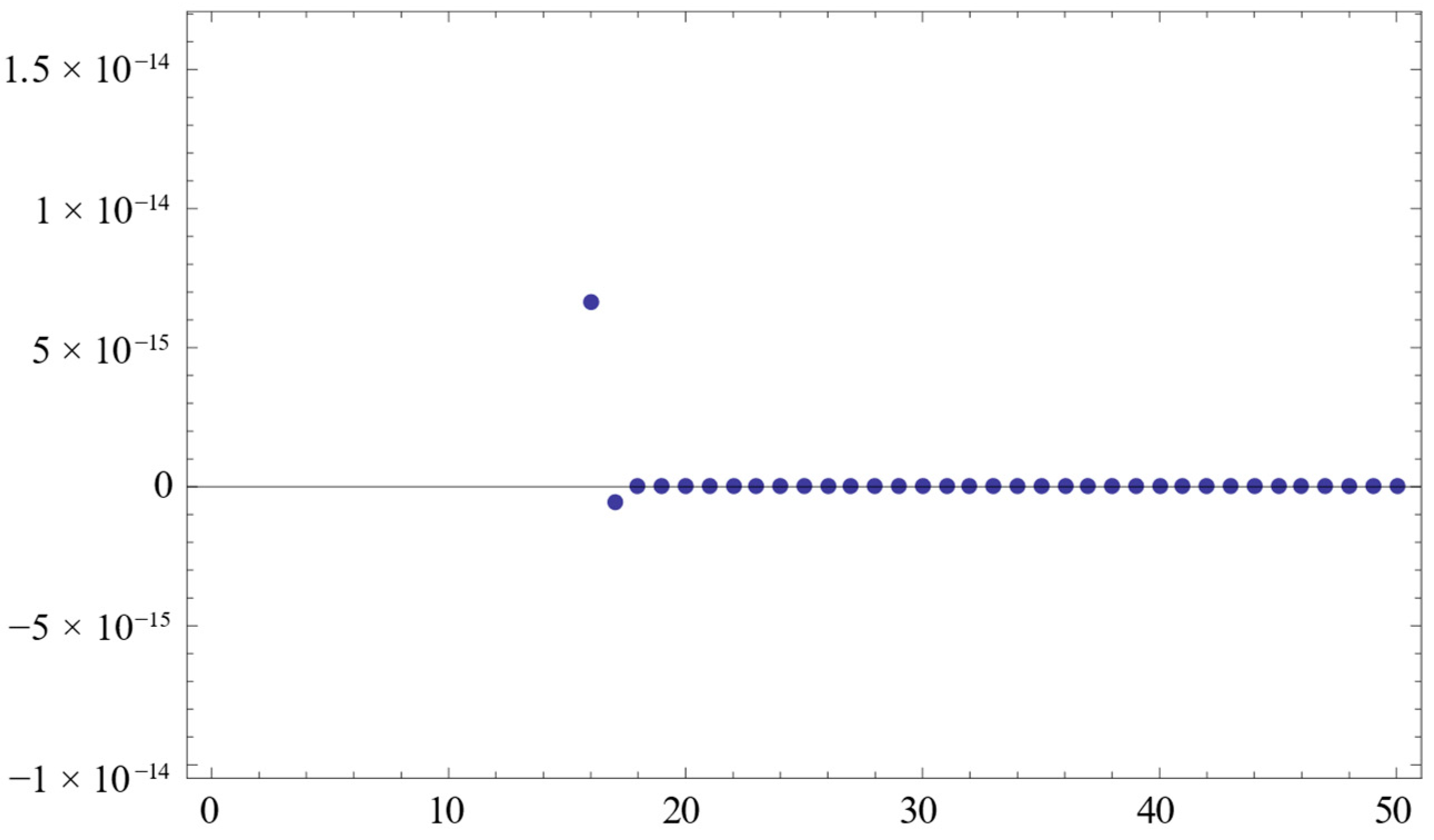
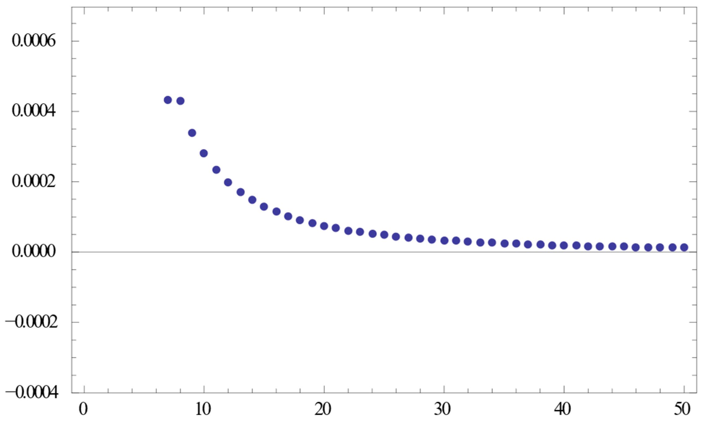
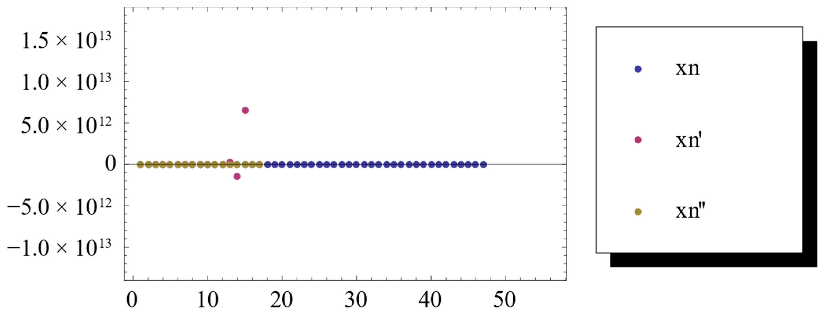
4. Numerical Examples

We provide some numerical examples to verify conclusions.
Example 1.
For any x R , assume  J r n x = r n x 3 ,  f ( x ) = x 7  and  S ( x ) = x 5 , then F ( S ) = { 0 } . Assume α n = 1 n , β n = n 2 n + 2 and r n = 1 1 n . From Theorem 1, they satisfy these conditions. { x n } is generated by (2). So we find that { x n } strongly converges to 0.
From (2), we have
x n + 1 = 21 n 3 + 51 n 2 + 30 n 203 n 3 + 210 n 2 + 21 n 14 x n .
Let x 1 = 1 in (10) and then we obtain the desired results; see Figure 1.
Example 2.
For any x R , assume J r n x = r n x 3 , f ( x ) = x 7 and S ( x ) = x 5 , then F ( S ) = { 0 } . Assume α n = 1 n , β n = n 2 n + 2 , r n = 1 1 n and e n = 1 n 2 . From Theorem 3, they satisfy these conditions. { x n } is generated by (6). So we find that { x n } strongly converges to 0.
From (6), we have
x n + 1 = 21 n 3 + 51 n 2 + 30 n 203 n 3 + 210 n 2 + 21 n 14 x n + n 3 3 n + 2 29 n 5 + 30 n 4 + 3 n 3 2 n 2
Next, let x 1 = 1 in (11) and then we obtain the desired results; see Figure 2.
Example 3.
The inner product , : R 3 × R 3 R is defined by
x , y = x 1 y 1 + x 2 y 2 + x 2 y 3 .
The usual norm  : R 3 R  is defined by
x = x 1 2 + x 2 2 + x 3 2 , x = ( x 1 , x 2 , x 3 ) R 3 .
For any  x R 3 , assume  J r n x = r n x 3 ,  f ( x ) = x 7  and  S ( x ) = x 5 , then  F ( S ) = { 0 } . Assume  α n = 1 n ,  β n = n 2 n + 2  and  r n = 1 1 n . From Theorem 1, they satisfy these conditions.  { x n }  is generated by (2). So we find that  { x n }  strongly converges to 0.
From (2), we have
x n + 1 = 21 n 3 + 51 n 2 + 30 n 203 n 3 + 210 n 2 + 21 n 14 x n .
Let x 1 = ( 1 , 2 , 3 ) in (12) and then we obtain the desired results; see Figure 3.
Example 4.
The inner product , : R 3 × R 3 R is defined by
x , y = x 1 y 1 + x 2 y 2 + x 2 y 3 .
The usual norm  : R 3 R  is defined by
x = x 1 2 + x 2 2 + x 3 2 , x = ( x 1 , x 2 , x 3 ) R 3 .
For any  x R 3 , assume  J r n x = r n x 3 ,  f ( x ) = x 7  and  S ( x ) = x 5 , then  F ( S ) = { 0 } . Assume  α n = 1 n ,  β n = n 2 n + 2 ,  r n = 1 1 n  and  e n = 1 n 2 . From Theorem 3, they satisfy these conditions.  { x n }  is generated by (6). So we find that  { x n }  strongly converges to 0.
From (6), we have
x n + 1 = 21 n 3 + 51 n 2 + 30 n 203 n 3 + 210 n 2 + 21 n 14 x n + n 3 3 n + 2 29 n 5 + 30 n 4 + 3 n 3 2 n 2 .
Let x 1 = ( 1 , 100 , 10 ) in (13) and then we obtain the desired results; see Figure 4.
Example 5.
Let { x n } be generated by Example 1. { x n } is generated by
y n = β n x n + x n + 1 2 + ( 1 β n ) J r n x n + x n + 1 2 , x n + 1 = α n f x n + ( 1 α n ) S y n .
{ x n }  is generated by
x n + 1 = α n f ( x n ) + ( 1 α n ) T s n x n + ( 1 s n ) x n + 1 .
And assume most of the conditions of Example 1 are satisfied except  β n = 1 n ,  s n = 1 1 n  and  T ( x ) = x 5 , so we obtain
x n + 1 = 3 9 n + 9 n 2 + 3 n 3 14 n 4 3 + 9 n 9 n 2 51 n 3 + 6 n 4 x n ,
and
x n + 1 = 2 4 n + 2 n 2 + n 3 6 n 2 2 n 3 x n ,
Let  x 1 = 1  in  { x n } ,  { x n }  and  { x n } , then we obtain the desired results; see Figure 5.
Figure 5 shows that iterative algorithm (2) has a faster convergence speed than the algorithm of Zhang [20,21]. The stability and effectiveness of iterative algorithm (2) are also better than the algorithm of Zhang [20,21].

5. Conclusions

In the paper, we propose a new iterative algorithm by using the generalized viscosity implicit midpoint rule and Banach space, which is also a symmetric space. Under some conditions, we find that the sequence strongly converges to a common point of the fixed point set of nonexpansive mapping and the zero point set of the accretive operator. Our work extends the results of Xu [17], Luo [18], Ke [19], Zhang [20] and Zhang [21]. In the end, we give five numerical examples and show that our algorithm can achieve faster convergence speed, stability and effectiveness. This work further extends and enriches the relevant theory of symmetric space. In this paper, we considered extending nonexpansive mapping to more general mappings, and will continue to research this issue to find better iterative algorithms.

Funding

This research received no external funding.

Data Availability Statement

Data are contained within the article.

Conflicts of Interest

The author declares no conflicts of interest.

References

  1. Chang, S.S.; Lee, H.W.J.; Chan, C.K. Strong convergence theorems by viscosity approximation methods for accretive mappings and nonexpansive mappings. J. Appl. Math. Inform. 2009, 27, 59–68. [Google Scholar]
  2. Jung, J.S.; Cho, Y.J.; Zhou, H.Y. Iterative processes with mixed errors for nonlinear equations with perturbed m-accretive operators in Banach spaces. Appl. Math. Comput. 2002, 133, 389–406. [Google Scholar] [CrossRef]
  3. Moudafi, A. Viscosity approximation methods for fixed points problems. J. Math. Anal. Appl. 2000, 241, 46–55. [Google Scholar] [CrossRef]
  4. Qin, X.L.; Cho, S.Y.; Wang, L. Iterative algorithms with errors for zero points of m-accretive Operators. Fixed Point Theory Appl. 2013, 2013, 148. [Google Scholar] [CrossRef]
  5. Reich, S. Approximating zeros of accretive operators. Proc. Am. Math. Soc. 1975, 51, 381–384. [Google Scholar] [CrossRef]
  6. Reich, S. On fixed point theorems obtained from existence theorems for differential equations. J. Math. Anal. Appl. 1976, 54, 26–36. [Google Scholar] [CrossRef]
  7. Auzinger, W.; Frank, R. Asymptotic error expansions for stiff equations: An analysis for the implicit midpoint and trapezoidal rules in the strongly stiff case. Numer. Math. 1989, 56, 469–499. [Google Scholar] [CrossRef]
  8. Bader, G.; Deuflhard, P. A semi-implicit mid-point rule for stiff systems of ordinary differential equations. Numer. Math. 1983, 41, 373–398. [Google Scholar] [CrossRef]
  9. Deuflhard, P. Recent progress in extrapolation methods for ordinary differential equations. SIAM Rev. 1985, 27, 505–535. [Google Scholar] [CrossRef]
  10. Schneider, C. Analysis of the linearly implicit mid-point rule for differential-algebra equations. Electron. Trans. Numer. Anal. 1993, 1, 1–10. [Google Scholar]
  11. Somalia, S. Implicit midpoint rule to the nonlinear degenerate boundary value problems. Int. J. Comput. Math. 2002, 79, 327–332. [Google Scholar] [CrossRef]
  12. Van Veldhuxzen, M. Asymptotic expansions of the global error for the implicit midpoint rule (stiff case). Computing 1984, 33, 185–192. [Google Scholar] [CrossRef]
  13. Hammad, H.A.; ur Rehman, H.; De la Sen, M. Accelerated modified inertial Mann and viscosity algorithms to find a fixed point of α—Inverse strongly monotone operators. AIMS Math. 2021, 6, 9000–9019. [Google Scholar] [CrossRef]
  14. Hammad, H.A.; ur Rehman, H.; Kattan, D.A. Strong convergence for split variational inclusion problems under hybrid algorithms with applications. Alex. Eng. J. 2024, 87, 350–364. [Google Scholar] [CrossRef]
  15. Jung, J.S. Strong convergence of an iterative algorithm for accretive operators and nonexpansive mappings. J. Nonlinear Sci. Appl. 2016, 9, 2394–2409. [Google Scholar] [CrossRef]
  16. Li, D.F. On nonexpansive and accretive operators in Banach spaces. J. Nonlinear Sci. Appl. 2017, 10, 3437–3446. [Google Scholar] [CrossRef]
  17. Xu, H.K.; Alghamdi, M.A.; Shahzad, N. The viscosity technique for the implicit midpoint rule of nonexpansive mappings in Hilbert spaces. Fixed Point Theory Appl. 2015, 2015, 41. [Google Scholar] [CrossRef]
  18. Luo, P.; Cai, G.; Shehu, Y. The viscosity iterative algorithms for the implicit midpoint rule of nonexpansive mappings in uniformly smooth Banach spaces. J. Inequal. Appl. 2017, 2017, 154. [Google Scholar] [CrossRef] [PubMed]
  19. Ke, Y.F.; Ma, C.F. The generalized viscosity implicit rules of nonexpansive mappings in Hilbert spaces. Fixed Point Theory Appl. 2015, 2015, 190. [Google Scholar] [CrossRef]
  20. Zhang, H.C.; Qu, Y.H.; Su, Y.F. Strong convergence theorems for fixed point problems for nonexpansive mappings and zero point problems for accretive operators using viscosity implicit midpoint rules in Banach spaces. Mathematics 2018, 6, 257. [Google Scholar] [CrossRef]
  21. Zhang, H.C.; Qu, Y.H.; Su, Y.F. The generalized viscosity implicit midpoint rule for nonexpansive mappings in Banach space. Mathematics 2019, 7, 512. [Google Scholar] [CrossRef]
  22. Filali, D.; Ali, F.; Akram, M.; Dilshad, M. A Novel Fixed-Point Iteration Approach for Solving Troesch’s Problem. Symmetry 2024, 16, 856. [Google Scholar] [CrossRef]
  23. Reich, S. On the asymptotic behavior of nonlinear semigroups and the range of accretive operators. J. Math. Anal. Appl. 1981, 79, 113–126. [Google Scholar] [CrossRef]
  24. Barbu, V. Nonlinear Semigroups and Differential Equations in Banach Spaces; Editura Academiei Republicii Socialiste Romania; Springer: Dordrecht, The Netherlands, 1976; Volume 2, pp. 1–6. [Google Scholar]
  25. Liu, L.S. Ishikawa and Mann iterative process with errors for nonlinear strongly accretive mappings in Banach spaces. J. Math. Anal. Appl. 1995, 194, 114–125. [Google Scholar] [CrossRef]
  26. Reich, S. Strong convergence theorems for resolvents of accretive operators in Banach spaces. J. Math. Anal. Appl. 1980, 75, 287–292. [Google Scholar] [CrossRef]
Figure 1. Numerical results.
Symmetry 16 01528 g001
Figure 2. Numerical results.
Symmetry 16 01528 g002
Figure 3. Numerical results.
Symmetry 16 01528 g003
Figure 4. Numerical results.
Symmetry 16 01528 g004
Figure 5. Numerical results.
Symmetry 16 01528 g005
Disclaimer/Publisher’s Note: The statements, opinions and data contained in all publications are solely those of the individual author(s) and contributor(s) and not of MDPI and/or the editor(s). MDPI and/or the editor(s) disclaim responsibility for any injury to people or property resulting from any ideas, methods, instructions or products referred to in the content.

