Article

Quantitative Analysis of Magnetic Force of Axial Symmetry Permanent Magnet Structure Using Hybrid Boundary Element Method

by
Ana Vučković
1,
Dušan Vučković
1,
Mirjana Perić
1 and
Branislav M. Ranđelović
1,2,*
1
Faculty of Electronic Engineering, University of Niš, 18000 Niš, Serbia
2
Faculty of Teachers Education, University of Priština in K. Mitrovica, 38218 Leposavić, Serbia
*
Author to whom correspondence should be addressed.
Symmetry 2024, 16(11), 1495; https://doi.org/10.3390/sym16111495
Submission received: 10 October 2024 / Revised: 27 October 2024 / Accepted: 6 November 2024 / Published: 8 November 2024
(This article belongs to the Section Engineering and Materials)

Abstract

:
This paper investigates the forces generated by axially magnetized ring permanent magnets with trapezoidal cross-sections when placed near a soft magnetic cylinder. Utilizing the Hybrid Boundary Element Method (HBEM), this study models interactions in magnetic configurations, aiming to improve force calculation efficiency and accuracy compared to traditional finite element methods (FEMM 4.2 software program). The influence of the permanent magnet and the soft magnetic cylinder is approximated with a system of thin toroidal sources on the surfaces of the magnet and the cylinder, which significantly reduces the computation time for the force calculation. The approach is validated by comparing results with FEM solutions, revealing high precision with a much faster computation. Additionally, this study explores the influence of various parameters, including magnet size, separation distance, and magnetic permeability of the cylinder, on the magnetic force. The results demonstrate that the HBEM approach is effective for analyzing complex magnetic configurations, particularly in applications requiring efficient parametric studies. This approach can be adapted for other geometries, such as truncated cones or rectangular cross-section ring magnets. The findings contribute valuable insights into designing efficient magnetic systems and optimizing force calculations for varied magnet geometries and configurations, including the atypical ones.

1. Introduction

Permanent magnets find extensive application in a diverse array of devices, contributing to their widespread use and varied functionalities [1,2,3,4]. They are commonly utilized in magnetic couplings and bearings, magnetic assemblies, sensors, motors, and actuators. Their adoption is driven by factors such as suitability for specific applications, device miniaturization, cost-effectiveness, and the ability to extend operational capacities beyond those achievable with conventional devices. As the demand for optimization and continuous improvement of devices persists, there is a growing emphasis on the development of methods for accurate determination [5,6].
Inspired by Earnshaw’s significant discovery from 1848 [7], the global community of scientists has been actively engaged in addressing this challenge, presenting various approaches for the calculation of the magnetic field and forces associated with permanent magnets [8,9,10,11]. Various techniques exist with the goal of achieving the most straightforward and rapid analysis of magnetic structures in relation to various parameters. Typically, analytical methods for calculating permanent magnet fields, which are based on the distribution of magnetic charges [5,6] or Ampere’s microscopic currents [12], are confined to block and cylindrical structures. To address the limitations of both analytical and numerical methods, numerous semi-numerical approaches have been introduced by different researchers. Additionally, numerous scholarly works delve into the intricacies of calculating the force between permanent magnets of arbitrary shapes and ideally soft magnetic plates in close proximity, leveraging the image method applied to magnetostatics [13].
The existing literature predominantly concentrates on field and force models of permanent magnets with cylindrical, cuboidal, or ring configurations [12,13,14,15,16]. Nevertheless, the potential for enhanced performance in many electromechanical devices prompts the consideration of alternative magnet shapes [17,18,19]. Nevertheless, cone-shaped and tapered designed permanent magnets find practical applications in various fields, including nuclear magnetic resonance (NMR), magnetometers, and sensor technology [17]. In light of this, this paper explores the dynamics of a permanent ring magnet with a trapezoidal cross-section, as it may have applications in these areas.
In the initial configuration under examination, a trapezoidal cross-section ring permanent magnet, magnetized along the axial direction, is situated in proximity to a cylindrical entity composed of linear magnetic material of constant magnetic permeability. Since magnetic assemblies consist of various housings and permanent magnets, which modify magnetic circuits to attain specific magnetic properties and enhance durability, the scenario discussed in this paper provides valuable insights for the design process of magnetic assemblies.
The Hybrid Boundary Element Method (HBEM), developed at the Department of Theoretical Electrical Engineering, Faculty of Electronic Engineering in Niš, Serbia [20,21,22,23,24,25], and applied in this paper for modeling permanent magnet configurations, offers a valuable tool for deriving forces when a permanent magnet interacts with a soft magnetic body of finite dimensions, especially efficient with symmetric configurations. This methodological approach adds depth to the understanding of the intricate interplay between a permanent magnet and its surrounding environment, shedding light on the forces at play in the proximity of a soft magnetic body.

2. Methodology

To date, the Hybrid Boundary Element Method (HBEM) has been applied to solve multilayer electromagnetic problems. It is applied in solving different permanent magnet configurations [16,22,23], various microstrip lines configurations [21,25], determining electromagnetic fields near cable terminations [20,24], grounding systems [26], and metamaterial structures [27].
In accordance with HBEM [20], the influence of different magnetic materials in the modeling of various permanent magnet systems could be replaced by placing equivalent magnetic sources on the boundary surfaces of two magnetic materials or the boundary between a magnetic material and the air. In that case, the equivalent magnetic sources would be positioned in vacuum.
For instance, a permanent magnet of arbitrary shape, magnetized in an arbitrary direction, is located in a multilayer magnetic material (Figure 1a). Let the magnetic permeabilities of the layers be μ1, μ2,…, μN, as shown in Figure 1a. Using the HBEM, the effect of a multilayer medium can be replaced with magnetic sources at the boundary between two magnetic materials (or the boundary between a magnetic material and air), positioned in a vacuum. A system equivalent to the considered configuration is presented in Figure 1b. In addition to these equivalent magnetic sources, considering that the permanent magnet with magnetization vector M exists, there are also fictitious surface magnetic charges at permanent magnet surfaces, and volume magnetic charges. Since these fictitious magnetic charges of the magnet can be determined based on the known magnetization vector M, the only unknowns in the formed system of equations are the sources placed at the boundary of the media.
The magnetic sources positioned along the material boundaries can be linear [20,21], toroidal [22,23], or point-like [16], depending on the configuration of the problem being solved. Given that this study analyzes an axially symmetric structure, thin toroidal magnetic sources will be placed on the boundary surface between the magnetic material and air.

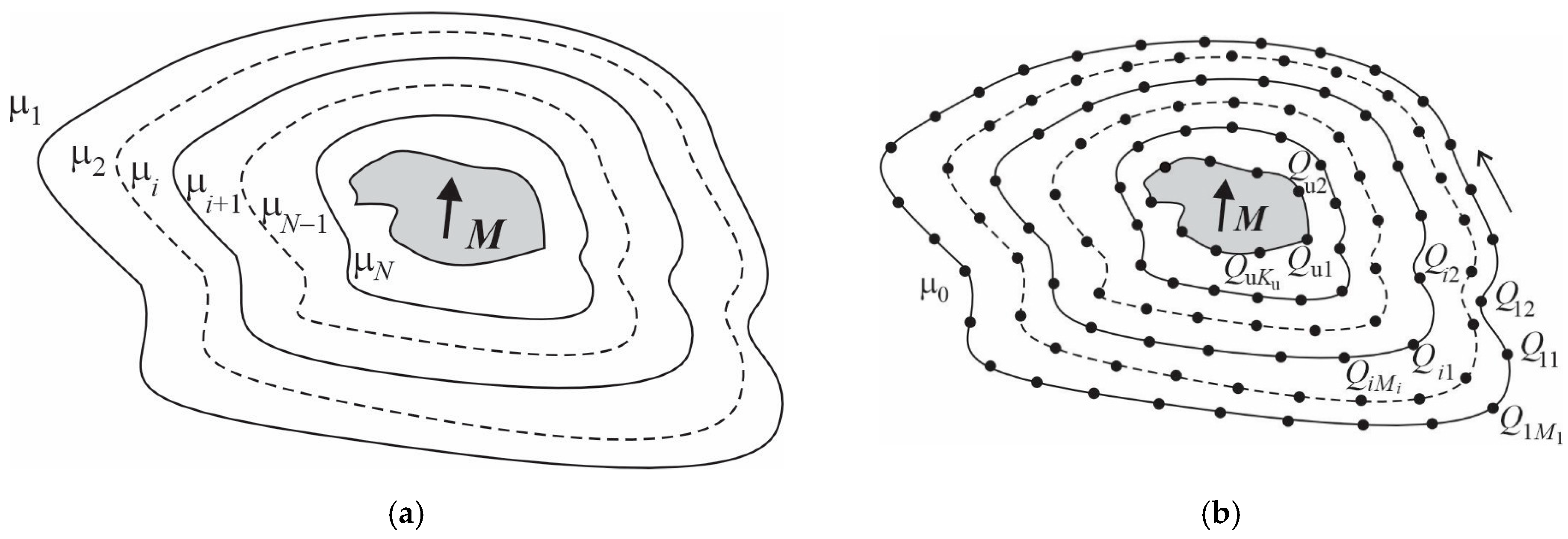
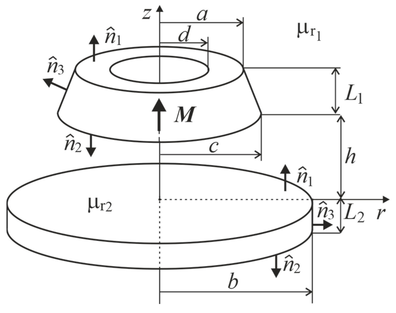
2.1. Problem Statement

A ring permanent magnet (PM) of trapezoidal cross-section is homogeneously magnetized in the axial direction, where the magnetization vector is M. It is placed above the cylinder made of linear magnetic material with constant relative magnetic permeability μ r 2 (soft magnetic cylinder) (Figure 2).
The distance between the magnet and the cylinder is denoted by h, and the radius of the cylinder by b, while its height is marked as L2. The inner radius of the magnet is d, its bottom outer radius is c, and a designates the top outer radius. The height of the magnet is L1.
To determine the force between the magnet and the cylinder made of linear magnetic material, it is first necessary to calculate the magnetic field strength vector (H) and magnetic flux density vector (B) in the vicinity of the system. According to the equation,
H = φ m
the magnetic scalar potential, φ m , should be determined first.
To achieve this, it is essential to create a system that is equivalent to the observed configuration.
Considering that relations between fictitious magnetic charges and magnetization vector are given by [28]
η m 1 = n ^ 1 M = M ,
η m 2 = n ^ 2 M = M ,
η m c = n ^ 3 M = M ( c a ) / ( c a ) 2 + L 1 2 ,
ρ m = M = 0 ,
the presence of surface magnetic charges is apparent on both ends of the magnet, η m 1 and η m 2 , as well as on its outer cover, η m c . Because of homogeneous and uniform axial magnetization of the magnet, the volume magnetic charges, ρ m , do not exist in this case. Employing a semi-analytical method rooted in the concept of fictitious magnetic charges [8], both the bases and the casing of the magnet are discretized into an array of circular loops, each carrying distinct magnetic charges.
The cylinder consists of a linear magnetic material characterized by its relative permeability, denoted as μ r 2 . Its impact on the permanent magnet mirrors the effect of an array of extremely slender toroidal magnetic sources positioned along the boundary surface of two distinct materials (the magnetic cylinder surface and the air). Refer to Figure 3 for details on the discretization model, magnetic charge distributions, and the configuration of thin toroidal sources.
Analyzing Figure 3, let us assume that N b 1 represents the number of discretization segments (circular loops) of the upper permanent magnet base. N b 2 is the number of discretization segments of lower permanent magnet base, while N c designates the number of cover segments. N b 1 , N b 2 , and N c are calculated from the initial number of surface segments, N s , and they depend on the permanent magnet dimensions. N 1 is the number of sources for each cylinder base, while N 2 is the number of cylinder cover sources. So, the total number of cylinder magnetic sources is N tot = 2 N 1 + N 2 .
The assignment of the segment count originates from the initial number of toroidal sources N and varies according to the dimensions of the cylinder.

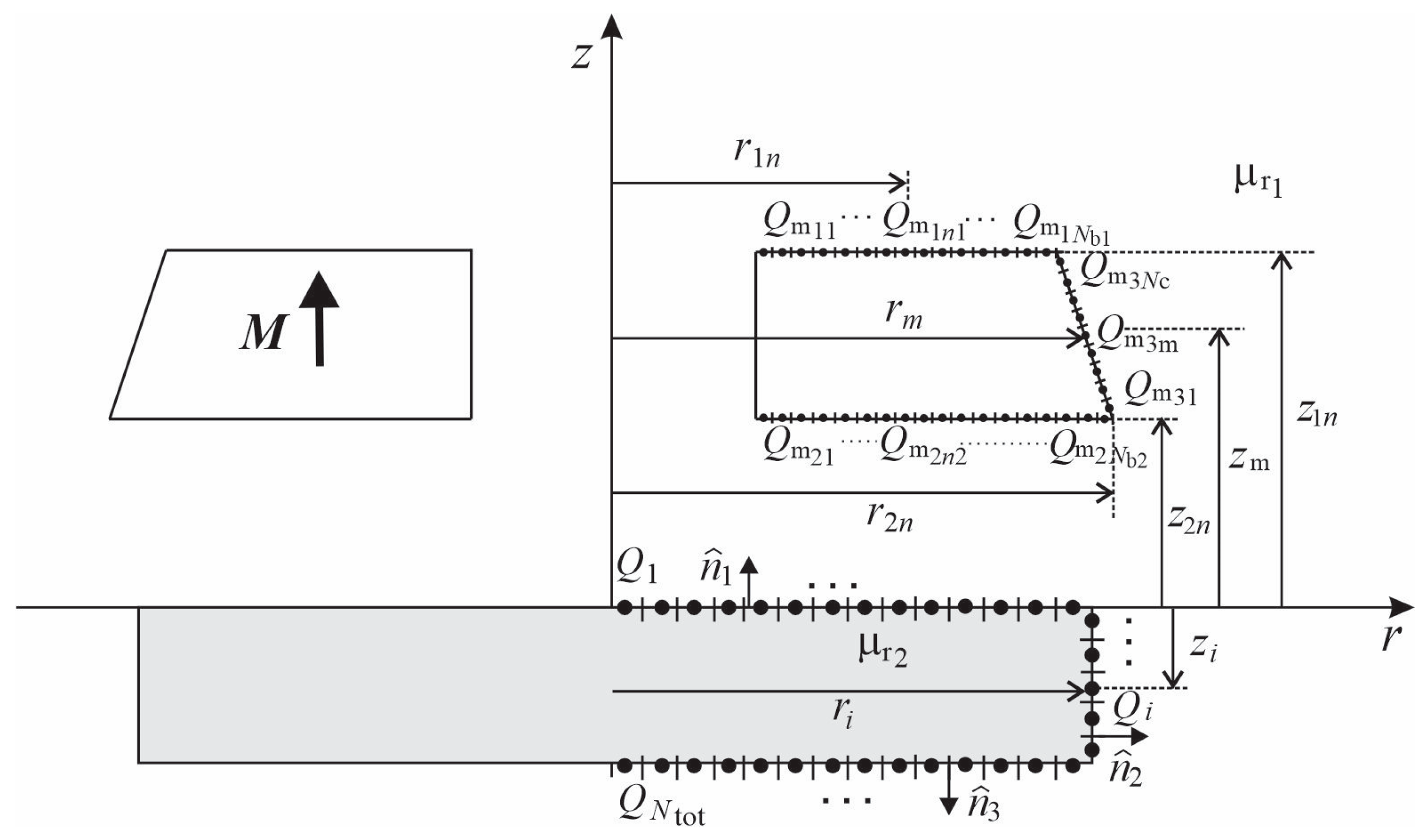
2.2. Determination of Magnetic Charges

Following the discretization process, the magnetic scalar potential of the system under consideration can be represented utilizing the equation derived in [8] for the magnetic scalar potential of a loop uniformly loaded with magnetic charge Q:
φ m ( r , z ) = 1 2 π 2 n 1 = 1 N b 1 Q m 1 n 1 K ( k 1 ) ( r + r n 1 ) 2 + ( z z n 1 ) 2 + n 2 = 1 N b 2 Q m 2 n 2 K ( k 2 ) ( r + r n 2 ) 2 + ( z z n 2 ) 2                      + m = 1 N c Q m 3 m K ( k 3 ) ( r + r m ) 2 + ( z z m ) 2 + i = 1 N tot Q i K ( k 4 ) ( r + r i ) 2 + ( z z i ) 2
where K ( k 1 ) , K ( k 2 ) , K ( k 3 ) , K ( k 4 ) are the complete elliptic integrals of the first kind with moduli k 1 2 = 4 r r n 1 ( r + r n 1 ) 2 + ( z z n 1 ) 2 , k 2 2 = 4 r r n 2 ( r + r n 2 ) 2 + ( z z n 2 ) 2 , k 3 2 = 4 r r m ( r + r m ) 2 + ( z z m ) 2 , k 4 2 = 4 r r i ( r + r i ) 2 + ( z z i ) 2 .
Parameters for the segments of the permanent magnet’s upper base encompass (Figure 3)
r n 1 = 2 n 1 1 2 N b 1 a d , n 1 = 1 , 2 , , N b 1 ,
z n 1 = h + L 1 ,
while the magnetic charges of the upper base are
Q m 1 n 1 = M 2 π r n 1 a d N b 1 ,       n 1 = 1 , 2 , , N b 1 .
The parameters of the PM’s lower base are
r n 2 = 2 n 2 1 2 N b 2 c d ,    n 2 = 1 , 2 , , N b 2 ,
z n 2 = h ,
while the magnetic charges of that base are
Q m 2 n 2 = M 2 π r n 2 c d N b 2 ,       n 2 = 1 , 2 , , N b 2 .
The corresponding parameters of PM’s cover segments are
r m = c c a L 1 ( z m h ) ,      m = 1 , 2 , , N c ,
z m = h + 2 m 1 2 N c L 1 ,     m = 1 , 2 , , N c ,
and magnetic charges of the cover are
Q m 3 m = M cos α 2 π r m ( c a ) 2 + L 1 2 N c ,   
where cos α = c a ( c a ) 2 + L 1 2 ,     m = 1 , 2 , , N c .
The positions of the toroidal magnetic sources along the cover and bases of the soft magnetic cylinder are denoted as r i , z i .
The positions of the sources along the upper base are
r i = 2 i 1 2 N 1 b ,    z i = 0 , i = 1 , 2 , , N 1 ,
while the cross-section radius of thin toroidal sources is
a e 1 = Δ r 1 π = b π N 1 .
For the cover cylinder’s sources, the following relations are fulfilled:
r i = b ,    z i = 2 N 1 2 i + 1 2 N 2 L 2 ,     i = N 1 + 1 , , N 1 + N 2 ,
with radius
a e 1 = Δ z 2 π = L 2 π N 2 ,
and for the lower base, the toroidal sources’ positions are
r i = 2 i 2 N 1 2 N 2 1 2 N 1 b ,     z i = L 2 ,       i = N 1 + N 2 + 1 , , 2 N 1 + N 2 ,
and the radius is a e 3 = a e 1
Based on an expression for magnetic scalar potential, the components of the magnetic field strength vector, H, can be determined using Equation (1).
The fundamental relation of HBEM, ref. [20], that has to be satisfied is
n ^ k H k ( 0 + ) = μ r 2 μ r 1 μ r 2 η m i    ,
η m i = Q i 2 r i π Δ r i ,    i = 1 , 2 , , N tot ,     k = 1 , 2 , 3 .
where n ^ k is the unit normal vector, ( n ^ 1 = z ^ , n ^ 2 = r ^ , n ^ 3 = z ^ ) (Figure 3).
We utilized the point matching method, specifically for the normal component of the magnetic field. This approach leads to the formation of a system of linear equations. Solving this system provides the values for the unknown charges of the thin toroidal sources, denoted as Q i , positioned on the cover and both bases of the soft magnetic cylinder.

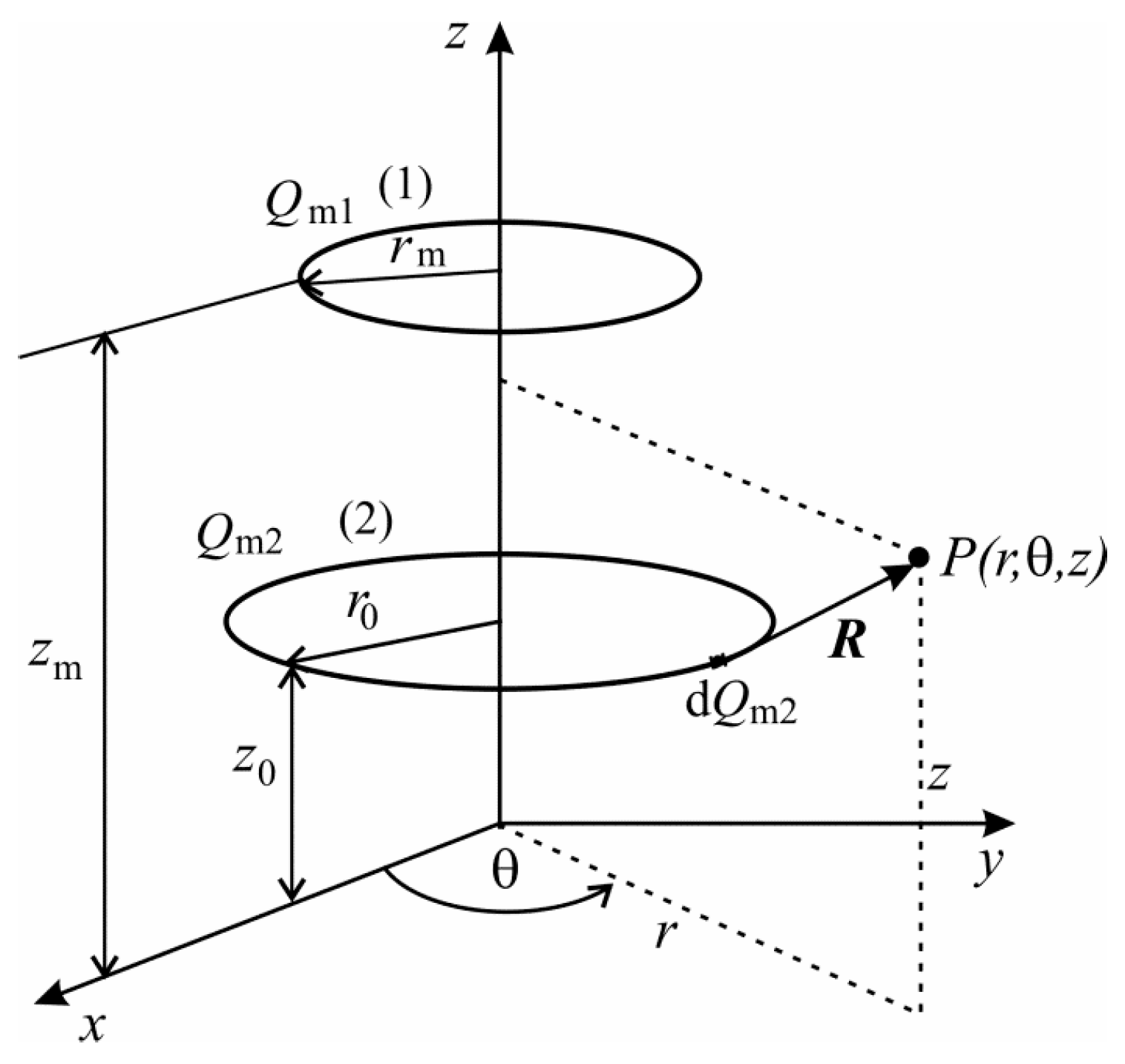
2.3. Force Calculation

Once the values of the unknown magnetic sources have been determined, the magnetic force acting between the permanent magnet (PM) and the soft magnetic cylinder can be computed by combining the results obtained for the axial magnetic force between two circular loops. This method, as outlined in reference [8], involves calculating the magnetic force between two circular loops (Figure 4) with varying magnetization charges distributed uniformly.
Magnetic force between two circular loops can be expressed as:
F z = μ 0 Q m 1 Q m 2 2 π 2 × z m z 0 E k 0 ( r m r 0 ) 2 + z m z 0 2 ( r m + r 0 ) 2 + z m z 0 2
where E k 0 is the complete elliptic integral of the second kind with modulus k 0 2 = 4 r 0 r m ( r m + r 0 ) 2 + ( z m z 0 ) 2 .
By summing up all contributions from the PM’s magnetic charges and toroidal magnetic sources, the resultant expression for the magnetic force can be derived.
F z = μ 0 2 π 2 n 1 = 1 N b 1 i = 1 N tot Q m 1 n 1 Q i P ( r n 1 , z n 1 , r i , z i ) + n 2 = 1 N b 2 i = 1 N tot Q m 2 n 2 Q i P ( r n 2 , z n 2 , r i , z i ) +                +    m = 1 N c i = 1 N tot Q m 3 m Q i P ( r m , z m , r i , z i )
where P ( r 0 , z 0 , r i , z i ) = ( z 0 z i ) E k i ( r 0 r i ) 2 + ( z 0 z i ) 2 ( r 0 + r i ) 2 + ( z 0 z i ) 2 and k i 2 = 4 r 0 r i ( r 0 + r i ) 2 + ( z 0 z i ) 2 .

3. Numerical Results

3.1. Comparison with FEMM

Using the derived expression (24), an analysis of the force is carried out parametrically, accompanied by graphical representation of the findings. The first part of the results analysis focuses on achieving convergence, determining the total count of permanent magnet segments, Ns, and the initial number of toroidal sources, N, as well as verifying the accuracy of the results.
To test the convergence, the normalized intensity of the magnetic force, F z nor = F z / μ 0 M 2 L 1 2 , is calculated for various numbers of permanent magnet and cylinder segments, considering parameters: a / L 1 = 2.0 ,   c / L 1 = 2.5 , d / L 1 = 1.0 ,   b / L 1 = 3.0 ,   L 2 / L 1 = 0.5 ,   h / L 1 = 0.5 ,   μ r 1 = 1 , μ r 2 = 10 , as shown in Table 1.
The FEMM 4.2 software program [29] is utilized to validate the accuracy of the results. For the mentioned parameters, the magnetic force using FEMM 4.2 is F z nor = 0.2964 . For all the values shown in Table 1, the relative error ranged from 0.6% to 0.03%. Notably, this method achieves high precision even with a limited number of magnetic sources. For instance, for N = N s = 50 , the relative error is 0.6%, and the computation time in that case is 0.98 s. In comparison, the time required in FEMM software for modeling such a system, adjusting parameters, setting up the mesh, running the program, and displaying the results (for approximately 700,000 nodes) takes around 5 min, which is nearly 300 times longer. Therefore, the time efficiency of the method is evident.
Although the error of 0.6%, obtained for N = N s = 50 , is acceptable for these parameters, in the case of larger permanent magnet and cylinder dimensions, a higher number of segments is required to ensure satisfactory accuracy (below 2%). For instance, when permanent magnet surface segments number is N s = 200 and the initial number of toroidal sources N = 200 , the relative deviation is 0.16%. It took around 4 s to compute, which is still significantly shorter than the time required to obtain a result using the FEMM software program.
For the parameters mentioned, the magnetic flux density distribution of the considered system is presented in Figure 5.
The distribution of calculated normalized magnetic charges, Q i nor = Q i / M L 1 2 , along the boundary surface of the cylinder and the air is presented in Figure 6. From point A to B, the distribution of magnetic sources along the upper base of the cylinder is shown. From point B to C, the distribution is presented along the cylinder’s lateral surface, and from C to D, the distribution of magnetic charges is shown along the lower base. It is determined for the following configuration parameters: a / L 1 = 3.0 ,   c / L 1 = 4.0 ,   d / L 1 = 1.0 ,   h / L 1 = 0.5 , L 2 / L 1 = 1.0 ,   b / L 1 = 3.0 ,   μ r 1 = 1 ,   μ r 2 = 50 , N s = 200 , and N = 500 . To confirm the accuracy of the applied approach once again, the force was calculated for these system parameters, yielding a value of F z nor = 0.338 . For the same parameters, using the FEMM software program, a value of F z nor = 0.335 was obtained, resulting in a relative error of 0.89%.

3.2. Parametric Studies of the Force

The values of the parameters for the permanent magnet and the cylinder that are considered in this analysis are illustrated in the figures. These parameters include dimensions such as height and diameter, distance between the magnet and cylinder, and material properties like relative magnetic permeability. All displayed force values are normalized, F z nor = F z / μ 0 M 2 L 1 2 , allowing the force to be calculated for any value of the magnetization vector intensity, M. In all upcoming analyses, the number of discretization segments for the permanent magnet is Ns = 200, and the number of segments for the cylinder is N = 200.
Figure 7 displays the comparative results for axial magnetic force as a function of the distance between the permanent magnet and the cylinder for various permanent magnet dimensions. The solid line represents the results obtained from the applied method, while the points indicate the outcomes from the FEMM software. For all the compared values, the relative deviation is less than 1%.
The axial magnetic force versus the distance between permanent magnet and cylinder, h / L 1 , is presented in Figure 8 for various values of cylinder radius.
Figure 9 presents the magnetic force versus relative permeability of the cylinder, μ r 2 , for different dimensions of the magnet, while Figure 10 illustrates the relationship between magnetic force and the relative permeability of a cylinder, showcasing how this relationship varies with different distances between the magnet and cylinder.
The axial magnetic force as a function of the relative magnetic permeability of the cylinder can be analyzed for different ratios of the cylinder’s height to the magnet’s height (Figure 11). This relationship reveals how changes in the magnetic properties of the cylinder and the geometric proportions between the magnet and the cylinder influence the magnetic force. In the case when d / L 1 = 0 , a truncated cone-shaped PM is obtained. For such a configuration, the magnetic force versus relative permeability of the cylinder is shown in Figure 12 for various axial displacement of permanent magnet, h / L 1 . With the selection of appropriate parameters, a ring permanent magnet with a rectangular cross-section can be formed. In that case, the axial magnetic force as a function of the distance between the magnet and the cylinder is calculated for different relative magnetic permeability values of the cylinder (Figure 13).
Figure 14 presents the comparative results for the force in the case of a permanent ring magnet with a trapezoidal cross-section and a rectangular cross-section of the same volume. The dependence of force is shown on distance h / L 1 for different values of radius c / L 1 , with the dimensions of the magnets a / L 1 and d / L 1 fixed. The curves are shown as solid lines in the figure. The same analysis was performed for the case of a magnet with a rectangular cross-section, calculated so that the volumes are identical. The force distribution is shown in the same figure with a dashed line. It can be observed that the force is marginally greater for the trapezoidal cross-section.

4. Discussion

Figure 7, Figure 8, Figure 13 and Figure 14 show the dependence of the normalized magnetic force on the normalized distance h / L 1 between the magnet and the cylinder. In Figure 8, the dependence is shown for different values of the cylinder’s radius. As expected, the larger the cylinder’s radius, the greater the force, but after the value b / L 1 = 4 , the increase in force becomes negligible for further increases in the cylinder’s radius. Figure 9, Figure 10 and Figure 11 analyze the dependence of force on the relative magnetic permeability of the cylinder for different values of the magnet’s inner radius, d / L 1 (Figure 9), varying distances between the magnet and the cylinder, h / L 1 (Figure 10), and different height ratios of the cylinder and the magnet, L 2 / L 1 (Figure 11). With an increase in the distance between the magnet and the cylinder, the force weakens. However, with an increase in relative magnetic permeability beyond 100, the force does not significantly change in intensity for certain dimensions of the magnet and the cylinder. This state is also demonstrated in Figure 13.
From Figure 9, it is evident that for smaller values of the magnet’s inner radius, d / L 1 the force intensity will also be greater since the magnet’s volume is larger in this case. Figure 11 shows that the height ratio of the magnet and the cylinder, L 2 / L 1 , has a significant impact on the force intensity when this ratio is less than one. However, when the ratio is equal to or greater than one, the curves showing the dependence of force on magnetic permeability do not differ significantly.
The obtained equation for the force is not restricted to the given geometry. It can also be used to calculate the force between truncated cone-shaped permanent magnet and soft magnetic cylinder (Figure 12) or between ring magnets with a rectangular cross-section and soft magnetic materials by properly adjusting the parameters (Figure 13).

5. Conclusions

The magnetic force between the soft magnetic cylinder and a trapezoidal cross-section axially magnetized ring permanent magnet (PM) is detailed in this paper. This derivation employs a semi-analytical method integrating magnetic charges and the Hybrid Boundary Element Method (HBEM). When applying HBEM, thin toroidal sources are introduced, resulting in a significantly smaller number of elements during the discretization technique. The efficiency of the method is also influenced by the use of an analytical expression for the force between two toroidal sources. The resulting expression is highly adaptable, facilitating straightforward implementation in standard software environments for thorough parametric analyses of the force. Notably, the approach’s reliability is confirmed by successful validation against finite element method (FEM) results, with an execution time approximately 300 times faster than that of the FEMM 4.2 software program. For more complex structures, the computational time is longer, but still much shorter than that obtained by the FEMM software program.
Furthermore, the method’s simplicity is evident, requiring only basic mathematical operations and the utilization of complete elliptical integrals of the second kind. This equation is not limited solely to the specified geometry; it can also be applied to different geometries with the appropriate adjustment of parameters.

Author Contributions

A.V.: methodology, software, validation, investigation, data curation, writing—original draft, and writing—review and editing. D.V.: software, visualization and writing—review and editing. M.P.: methodology, validation and writing—review and editing. B.M.R.: visualization and writing—review and editing. All authors have read and agreed to the published version of the manuscript.

Funding

This research was funded by Ministry of Science and technological developement of Republic Serbia grant number 451-03-65/2024-03/200102 and 451-03-65/2024-03/200251.

Data Availability Statement

The data used in this study are available in the article.

Conflicts of Interest

The authors declare no conflict of interest.

References

  1. Cavallaro, S.P.; Venturini, S.; Bonisoli, E. Nonlinear dynamics of a horizontal rotor with asymmetric magnetic supports. Int. J. Non-Linear Mech. 2024, 165, 104764. [Google Scholar] [CrossRef]
  2. Bernad, S.I.; Bernad, E. Magnetic Forces by Permanent Magnets to Manipulate Magnetoresponsive Particles in Drug-Targeting Applications. Micromachines 2022, 13, 1818. [Google Scholar] [CrossRef] [PubMed]
  3. Nemoianu, I.V.; Dragomirescu, C.G.; Manescu, V.; Dascalu, M.I.; Paltanea, G.; Ciuceanu, R.M. Self-Organizing equilibrium patterns of multiple permanent magnets floating freely under the action of a central attractive magnetic force. Symmetry 2022, 14, 795. [Google Scholar] [CrossRef]
  4. Zhang, X.; Zhang, M.; Jiao, S.; Zhang, X.; Li, M. Optimization design and parameter analysis of a wheel with array magnets. Symmetry 2023, 15, 962. [Google Scholar] [CrossRef]
  5. Ravaud, R.; Lemarquand, G.; Lemarquand, V. Force and stiffness of passive magnetic bearings using permanent magnets. Part 1: Axial magnetization. IEEE Trans. Magn. 2009, 45, 2996–3002. [Google Scholar] [CrossRef]
  6. Ravaud, R.; Lemarquand, G.; Lemarquand, V. Force and stiffness of passive magnetic bearings using permanent magnets. Part 2: Radial magnetization. IEEE Trans. Magn. 2009, 45, 3334–3342. [Google Scholar] [CrossRef]
  7. Earnshaw, S. On the nature of the molecular forces which regulate the constitution of the luminiferous ether. Trans. Camb. Philos. Soc. 1842, 7, 97–112. [Google Scholar]
  8. Vučković, A.N.; Raičević, N.B.; Ilić, S.S.; Aleksić, S.R. Interaction magnetic force calculation of radial passive magnetic bearing using magnetization charges and discretization technique. Int. J. Appl. Electromagn. Mech. 2013, 43, 311–323. [Google Scholar] [CrossRef]
  9. Robertson, W.S.; Cazzolato, B.S.; Zander, A.C. A Simplified force equation for coaxial cylindrical magnets and thin coils. IEEE Trans. Magn. 2011, 47, 2045–2049. [Google Scholar] [CrossRef]
  10. Yang, W.; Zhou, G.; Gong, K.; Li, Y. The numeric calculation for cylindrical magnet’s magnetic flux intensity. Int. J. Appl. Electromagn. Mech. 2012, 40, 227–235. [Google Scholar] [CrossRef]
  11. Rakotoarison, H.L.; Yonnet, J.P.; Delinchant, B. Using Coulombian approach for modeling scalar potential and magnetic field of a permanent magnet with radial polarization. IEEE Trans. Magn. 2007, 43, 1261–1264. [Google Scholar] [CrossRef]
  12. Vučković, A.N.; Ilić, S.S.; Aleksić, S.R. Interaction magnetic force calculation of ring permanent magnets using Ampere’s microscopic surface currents and discretization technique. Electromagnetics 2012, 32, 117–134. [Google Scholar] [CrossRef]
  13. Beleggia, M.; Vokoun, D.; Graef, M.D. Forces between a permanent magnet and a soft magnetic plate. IEEE Magn. Lett. 2012, 3, 0500204. [Google Scholar] [CrossRef]
  14. Akoun, G.; Yonnet, J.P. 3D analytical calculation of the forces exerted between two cuboidal magnets. IEEE Trans. Magn. 1984, 20, 1962–1964. [Google Scholar] [CrossRef]
  15. Furlani, E.P.; Reznik, S.; Kroll, A. A three-dimensional field solution for radially polarized cylinders. IEEE Trans. Magn. 1995, 31, 844–851. [Google Scholar] [CrossRef]
  16. Vučković, A.N.; Perić, M.T.; Ilić, S.S.; Raičević, N.B.; Vučković, D.M. Interaction magnetic force of cuboidal permanent magnet and soft magnetic bar using hybrid boundary element method. ACES J. 2021, 36, 1492–1498. [Google Scholar] [CrossRef]
  17. Hart, S.; Hart, K.; Selvaggi, J.P. Analytical expressions for the magnetic field from axially magnetized and conically shaped permanent magnets. IEEE Trans. Magn. 2020, 56, 7. [Google Scholar] [CrossRef]
  18. O’Connell, J.L.G.; Robertson, W.S.P.; Cazzolato, B.S. Analytic magnetic fields and semi-analytic forces and torques due to general polyhedral permanent magnets. IEEE Trans. Magn. 2020, 56, 7400208. [Google Scholar] [CrossRef]
  19. Vučković, A.; Vučković, D.; Perić, M.; Raičević, N. Magnetic force calculation between truncated cone-shaped permanent magnet and soft magnetic cylinder using hybrid boundary element method. In Stochastic Processes, Statistical Methods, and Engineering Mathematics; Springer Proceedings in Mathematics & Statistics; Springer International Publishing: Cham, Switzerland, 2022; Chapter 32; pp. 719–733. ISSN 2194-1009. ISBN 978-3-031-17819-1. [Google Scholar]
  20. Raičević, N.B.; Aleksić, S.R.; Ilić, S.S. A hybrid boundary element method for multilayer electrostatic and magnetostatic problems. Electromagnetics 2010, 30, 507–524. [Google Scholar] [CrossRef]
  21. Perić, M.T.; Ilić, S.S.; Aleksić, S.R.; Raičević, N.B. Characteristic parameters determination of different striplines configurations using HBEM. ACES J. 2013, 28, 858–865. [Google Scholar]
  22. Vučković, A.; Vučković, D.; Perić, M.; Raičević, N. Influence of the magnetization vector misalignment on the magnetic force of permanent ring magnet and soft magnetic cylinder. Int. J. Appl. Electromagn. Mech. 2021, 26, 417–430. [Google Scholar] [CrossRef]
  23. Vučković, A.N.; Raičević, N.B.; Perić, M.T. Radially magnetized ring permanent magnet modelling in the vicinity of soft magnetic cylinder. Saf. Eng. 2018, 8, 33–37. [Google Scholar] [CrossRef]
  24. Raičević, N.B.; Ilić, S.S.; Aleksić, S.R. Application of new hybrid boundary element method on the cable terminations. In Proceedings of the 14th International IGTE’10 Symposium, Graz, Austria, 20–22 September 2010; pp. 56–61. [Google Scholar]
  25. Perić, M.T.; Ilić, S.S.; Aleksić, S.R.; Raičević, N.B. Application of Hybrid boundary element method to 2D microstrip lines analysis. Int. J. Appl. Electromagn. Mech. 2013, 42, 179–190. [Google Scholar] [CrossRef]
  26. Ilić, S.S.; Raičević, N.B.; Aleksić, S.R. Application of new hybrid boundary element method on grounding systems. In Proceedings of the 14th International IGTE’10 Symposium, Graz, Austria, 20–22 September 2010; pp. 160–165. [Google Scholar]
  27. Raičević, N.B.; Ilić, S.S. One hybrid method application on complex media strip lines determination. In Proceedings of the 3rd International Congress on Advanced Electromagnetic Materials in Microwaves and Optics, Metamaterials, London, UK, 30 August–4 September 2009; pp. 698–700. [Google Scholar]
  28. Rovers, J.M.M.; Jansen, J.W.; Lomonova, E.A. Modeling of relative permeability of permanent magnet material using magnetic surface charges. IEEE Trans. Magn. 2013, 49, 2913–2919. [Google Scholar] [CrossRef]
  29. Meeker, Software Package FEMM 4.2. Available online: http://www.femm.info/wiki/Download (accessed on 2 March 2007).
Figure 1. (a) Permanent magnet in multilayer magnetic material; (b) equivalent HBEM system.
Symmetry 16 01495 g001
Figure 2. Toroidal permanent magnet placed above soft magnetic cylinder.
Symmetry 16 01495 g002
Figure 3. Discretization model.
Symmetry 16 01495 g003
Figure 4. Two circular loops.
Symmetry 16 01495 g004
Figure 5. Magnetic flux density distribution.
Symmetry 16 01495 g005
Figure 6. Magnetic sources distribution along the cylinder surface.
Symmetry 16 01495 g006
Figure 7. Comparative results for axial magnetic force versus distance between the magnet and cylinder, h / L 1 , for different dimensions of the magnet.
Symmetry 16 01495 g007
Figure 8. Axial magnetic force versus distance between the magnet and cylinder, h / L 1 , for different dimension of the cylinder.
Symmetry 16 01495 g008
Figure 9. Axial magnetic force versus relative magnetic permeability of the cylinder for various values of the inner PM radius.
Symmetry 16 01495 g009
Figure 10. Axial magnetic force versus relative magnetic permeability of the cylinder for various values of distance between magnet and cylinder.
Symmetry 16 01495 g010
Figure 11. Axial magnetic force versus relative magnetic permeability of the cylinder for various values of the ratio between the magnet and the cylinder heights.
Symmetry 16 01495 g011
Figure 12. Axial magnetic force versus relative magnetic permeability of the cylinder for various values of axial displacement, h / L 1 .
Symmetry 16 01495 g012
Figure 13. Axial magnetic force versus distance between the magnet and cylinder, h / L 1 , for relative magnetic permeability of the cylinder when torus is for rectangular cross-section.
Symmetry 16 01495 g013
Figure 14. Axial magnetic force versus distance between the magnet and cylinder, h / L 1 , for trapezoidal cross/section of the magnet (bold line) and rectangular cross-section of same volume (dashed line).
Symmetry 16 01495 g014
Table 1. Convergence of results for magnetic force, F z nor .
NS50100200300400500600
N
500.29820.29800.29790.29790.29790.29790.2979
1000.29770.29740.29730.29730.29730.29730.2973
2000.29730.29700.29690.29690.29690.29690.2969
3000.29710.29680.29680.29680.29670.29670.2967
4000.29700.29670.29670.29670.29660.29660.2966
5000.29690.29670.29660.29660.29660.29660.2966
6000.29690.29660.29660.29650.29650.29650.2965
Disclaimer/Publisher’s Note: The statements, opinions and data contained in all publications are solely those of the individual author(s) and contributor(s) and not of MDPI and/or the editor(s). MDPI and/or the editor(s) disclaim responsibility for any injury to people or property resulting from any ideas, methods, instructions or products referred to in the content.

