Analysis of COVID-19’s Dynamic Behavior Using a Modified SIR Model Characterized by a Nonlinear Function

Abstract

This study develops a modified SIR model (Susceptible–Infected–Recovered) to analyze the dynamics of the COVID-19 pandemic. In this model, infected individuals are categorized into the following two classes: $I_a$, representing asymptomatic individuals, and $I_s$, representing symptomatic individuals. Moreover, accounting for the psychological impacts of COVID-19, the incidence function is nonlinear and expressed as $Sg(I_a,I_s)={\displaystyle \frac{\beta S(I_a+I_s)}{1+\alpha (I_a+I_s)}}$. Additionally, the model is based on a symmetry hypothesis, according to which individuals within the same compartment share common characteristics, and an asymmetry hypothesis, which highlights the diversity of symptoms and the possibility that some individuals may remain asymptomatic after exposure. Subsequently, using the next-generation matrix method, we compute the threshold value ($R_0$), which estimates contagiousness. We establish local stability through the Routh–Hurwitz criterion for both disease-free and endemic equilibria. Furthermore, we demonstrate global stability in these equilibria by employing the direct Lyapunov method and La-Salle’s invariance principle. The sensitivity index is calculated to assess the variation of $R_0$ with respect to the key parameters of the model. Finally, numerical simulations are conducted to illustrate and validate the analytical findings.

1. Introduction

The highly contagious viral infection known as COVID-19 began in Wuhan, China, in December 2019 and quickly spread around the world. Therefore, understanding the transmission mechanisms and dynamic behavior of such infectious diseases is crucial. Epidemic models are a vital means to express the spread of infectious diseases. The incidence function plays a significant role in understanding the dynamics of infectious diseases, which have historically been modeled as bilinear in the form of $\left(\beta SI\right)$, where S represents the susceptible population, I indicates the infectious population, and $\beta$ is the contact rate. This approach is well documented in the literature [1,2,3]. However, bilinear incidence functions do not account for the effects of intervention strategies such as self-isolation, quarantine, social distancing, and vaccination, which can significantly alter the contact rates between susceptible and infected individuals.

Therefore, to control the spread of the disease, the adoption of a nonlinear incidence function more accurately reflects these various parameters, thereby enabling the development of effective strategies such as isolation, quarantine, and mask wearing while also reducing the efficacy of transmission. For instance, Shao and Shateyi [4] adopted an incidence function expressed as $\beta Sf\left(I\right)={\displaystyle \frac{\beta SI}{1+aI}}$ in their study. Various nonlinear incidence functions have also been examined [5,6,7,8,9,10].

Various mathematical models have been established to explore COVID-19 for multiple purposes. For example, Askar [11] introduced a fractional-order SITR model to investigate COVID-19 epidemics in India, while Alshammari and Khan [12] focused on analyzing a modified SIR model with nonlinear incidence. In parallel, Ali et al. [13] and Awais [14] used fractional-order models to study COVID-19 dynamics in Pakistan. Similarly, Basnarkov [15] analyzed a SEAIR model, while Kumar et al. [16] proposed a modified SIR model with a non-monotonic incidence function for COVID-19 transmission in India. Other notable studies include [17,18,19,20,21,22,23,24,25,26,27,28,29,30,31,32,33,34,35,36,37].

Adapting epidemiological models to capture the unique characteristics of COVID-19 is crucial for improving their predictive accuracy and effectiveness in public health strategies. Various authors have created mathematical models of COVID-19 for diverse purposes and approaches. Given that asymptomatic individuals play a significant role in the virus’s transmission, distinguishing between symptomatic and asymptomatic populations within the infected compartment provides a more precise understanding of the virus’s progression. SEIR models, which assume that infected individuals in the incubation period cannot transmit the disease, are also unsuitable for COVID-19, where asymptomatic individuals are infectious during this period. Traditional SIS and SIR models do not consider asymptomatic individuals, despite estimates suggesting that $78\%$ of COVID-19 cases are asymptomatic [38,39]. The relatively short incubation period (around 5.2 days) and the recommended 14-day quarantine make SIS and SIR models inadequate for COVID-19 scenarios. Kumar et al. [16] investigated the dynamics of COVID-19 in India through the use of an SIR model that classifies infected individuals into known and unknown groups, under the assumption that known individuals are isolated and do not propagate the disease. In a similar manner, Tomochi and Kono [40] constructed a modified SIR model that differentiates between symptomatic and asymptomatic individuals, effectively capturing the intricacies of COVID-19 transmission. Other research has utilized modified SIR models to enhance comprehension of COVID-19 dynamics [40,41,42,43,44,45].

In our analysis, we adopt an SIR model in which the infected compartment is divided into symptomatic and asymptomatic categories, featuring a nonlinear incidence rate. This methodology enables us to more thoroughly explore the complexities associated with disease propagation. This study focuses on assessing the stability of a modified SIR model with a nonlinear incidence function ($Sg(I_a,I_s)={\displaystyle \frac{\beta S(I_a+I_s)}{1+\alpha (I_a+I_s)}}$), as introduced by Mawlili et al. [46], where $I_a$ and $I_s$ are the asymptomatic and symptomatic populations and $\alpha$ is the saturation constant. Moreover, the term $1+\alpha (I_a+I_s)$ reflects an inhibitory influence that represents the role of precautionary measures in mitigating disease transmission. This model differs from the $\left(S{I}_u{I}_{k}R\right)$ model studied in [16], where only unknown infected individuals contribute to disease spread. It is also distinct from models proposed by Ottaviano et al. [43] and Essak and Boukanjime [44], who considered a (SAIRS) model with a bilinear incidence function ($({\beta }_{A}A+{\beta }_{I}I)$), assuming that asymptomatic individuals do not transmit the disease and can become symptomatic or recover directly. Another aspect of this study is a sensitivity analysis, which explores the impact of the parameters on $R_0$, reflecting the speed of spread of the disease. This analysis makes it possible to identify the essential parameters and provides decision makers with crucial information to adjust the main transmission factors [47].

The rest of this document is structured as follows: In Section 2, we develop a mathematical model to study the transmission of COVID-19. In Section 3, we examine the basic properties of the proposed model. Next, we calculate the basic reproduction number $\left(R_0\right)$. We finish this section with the proof of the local and global asymptotic stability of the equilibria. A sensitivity analysis of $R_0$ with respect to the key parameters of the system is conducted in Section 4. In Section 5, numerical simulations are performed to confirm the analytical results. Finally, in Section 6 and Section 7, we conclude this work with a discussion and conclusions encapsulating the results of this study.

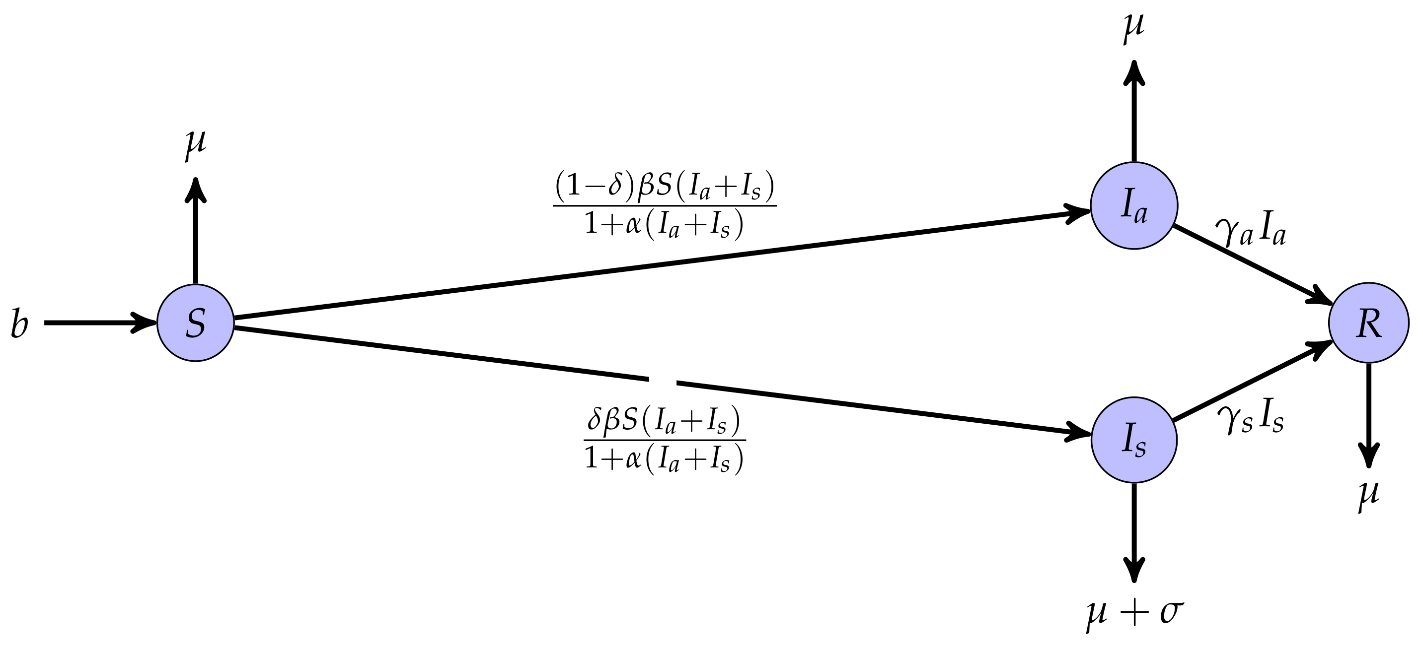
2. Formulation of COVID-19 Mathematical Model

This study presents a mathematical model to elucidate the transmission dynamics and spread of COVID-19, as illustrated in Figure 1.

Figure 1. Schematic representation of the model proposed in this study.

The total population (N) is classified into the following four specific groups: susceptible individuals (S), the asymptomatic population ($I_a$), the symptomatic population ($I_s$), and recovered individuals (R). Parameters of the COVID-19 pandemic model are listed in the Table 1.

Table 1. Parameters of the COVID-19 pandemic model.

Parameter	Description
b	Rate of population recruitment
$\beta$	Rate of disease transmission from susceptible individuals (S) to infected compartments ($I_a$ and $I_s$)
$\alpha$	Constant of saturation reflecting psychological or inhibitory effects on the transmission of infection
$\delta$	Rate of susceptible individuals who develop symptoms of the disease
${\gamma }_a$	Rate of recovery from the asymptomatic population to the recovered population
${\gamma }_s$	Rate of recovery from the symptomatic population to the recovered population
$\sigma$	Mortality rate attributed to COVID-19
$\mu$	Rate of natural mortality

The modified SIR model is illustrated Figure 1 based on the following specific epidemiological assumptions related to the COVID-19 pandemic:

1.

Symmetrical assumption: In this model, the capacity for virus transmission is identical for infected individuals, whether symptomatic or asymptomatic. Thus, groups $I_a$ (asymptomatic individuals) and $I_s$ (symptomatic individuals) are treated identically, following a common path to recovery with different transmission rates (${\gamma }_a{I}_a$ for asymptomatic individuals and ${\gamma }_s{I}_s$ for symptomatic individuals).

2.

Asymmetrical assumption: The response to the virus varies among individuals; some develop symptoms, while others remain asymptomatic, creating an asymmetry in transmission. A certain percentage of the susceptible population develops symptoms ($\delta Sg(I_a,I_s)={\displaystyle \frac{\delta \beta S(I_a+I_s)}{1+\alpha (I_a+I_s)}}$), while another percentage becomes asymptomatic ($\delta Sg(I_a,I_s)={\displaystyle \frac{\delta \beta S(I_a+I_s)}{1+\alpha (I_a+I_s)}}$).

3.

Natural mortality: Natural mortality affects all compartments of the model and represents a shared biological constant. Unlike the symmetrical and asymmetrical assumptions, this mortality does not distinguish between individuals based on their infectious status but reflects a universal biological reality.

The model proposed in this research is formulated as the following system of nonlinear ordinary differential equations:

$$\left\{\begin{array}{c}\begin{array}{cc}\hfill & {\displaystyle \frac{dS\left(t\right)}{dt}}=b-{\displaystyle \frac{\beta S(I_a+I_s)}{1+\alpha (I_a+I_s)}}-\mu S,\hfill \\ \hfill & {\displaystyle \frac{d{I}_a\left(t\right)}{dt}}={\displaystyle \frac{(1-\delta )\beta S(I_a+I_s)}{1+\alpha (I_a+I_s)}}-(\mu +{\gamma }_a)I_a,\hfill \\ \hfill & {\displaystyle \frac{d{I}_s\left(t\right)}{dt}}={\displaystyle \frac{\delta \beta S(I_a+I_s)}{1+\alpha (I_a+I_s)}}-(\mu +\sigma +{\gamma }_s)I_s,\hfill \\ \hfill & {\displaystyle \frac{dR\left(t\right)}{dt}}={\gamma }_a{I}_a+{\gamma }_s{I}_s-\mu R,\hfill \end{array}\hfill \end{array}\right.$$

(1)

with the following initial states:

$$S\left(0\right)>0,I_a\left(0\right)>,I_s\left(0\right)>, \mathrm{and} R\left(0\right)>0.$$

(2)

3. Results

We begin this section by proving some fundamental properties of the model. Then, we establish that the model admits the following two equilibria: a disease-free equilibrium and an endemic equilibrium. According the values of the basic reproduction number ($R_0$), we show that these equilibria are locally and globally asymptotically stable.

3.1. Principal Properties of the Model

The primary objective is to explore the essential characteristics of the model.

3.1.1. Analysis of the Positivity of the Solutions

Proposition 1.

Every solution of the system (3) maintains positivity for all values of time (t).

Proof of Proposition 1.

Based on the first equation in system (1), it follows that

$${\displaystyle \frac{dS\left(t\right)}{dt}}>-\left(\mu +{\displaystyle \frac{\beta (I_a\left(t\right)+I_s\left(t\right))}{1+\alpha (I_a\left(t\right)+I_s\left(t\right))}}\right)S\left(t\right).$$

By integrating this inequality, considering the function $\varphi \left(x\right)=\mu +{\displaystyle \frac{\beta x}{1+\alpha x}}$ and since $S\left(0\right)>0$, we arrive at the conclusion that

$$S\left(t\right)>S\left(0\right)e^{-{\int }_0^t\varphi (I_a\left(u\right)+I_s\left(u\right))du}>0.$$

Based on the second and third equations of system (1), we conclude that $I_a\left(0\right)\ge 0,$$I_s\left(0\right)\ge 0$,

$$I_a\left(t\right)\ge I_a\left(0\right)e^{-(\mu +{\gamma }_a)t}\ge 0\mathrm{a}\mathrm{n}\mathrm{d}{I}_s\left(t\right)\ge I_s\left(0\right)e^{-(\mu +\sigma +{\gamma }_s)t}\ge 0.$$

Consequently, from the final equation of system (1), we derive $R\left(0\right)\ge 0$ and $R\left(t\right)\ge R\left(0\right)e^{-\mu t}\ge 0.$

In conclusion, we establish that for every $t\ge 0$, $S\left(t\right)>0$, $I_a\left(t\right)\ge 0$, $I_s\left(t\right)\ge 0$, and $R\left(t\right)\ge 0$. □

3.1.2. Invariant Domain

Proposition 2.

The admissible domain (Ω), as detailed below, demonstrates positive invariance for system (1) as follows:

$$\begin{array}{c}\hfill \Omega =\left\{\left(S\left(t\right),I_a\left(t\right),I_s\left(t\right),R\left(t\right)\right)\in {\mathbb{R}}_{+}^4\mid S\left(t\right)+I_a\left(t\right)+I_s\left(t\right)+R\left(t\right)\le {\displaystyle \frac{b}{\mu }},t\ge 0\right\}.\end{array}$$

Proof of Proposition 2.

Consider $\left(S\left(t\right),I_a\left(t\right),I_s\left(t\right),R\left(t\right)\right)$ as a solution to system (1), with initial conditions of $\left(S\left(0\right),I_a\left(0\right),I_s\left(0\right),R\left(0\right)\right)\in \Omega$; then, we obtain

$$\begin{array}{ccc}\hfill {\displaystyle \frac{dN\left(t\right)}{dt}}& =& b-\mu N\left(t\right)-\sigma I_s\left(t\right),\hfill \\ & \le & b-\mu N\left(t\right),\hfill \end{array}$$

where $N\left(t\right)=S\left(t\right)+I_a\left(t\right)+I_s\left(t\right)+R\left(t\right)$. Therefore, ${\displaystyle \frac{dN\left(t\right)}{dt}}+\mu N\left(t\right)\le b$, and by applying the standard comparison theorem [48,49], we conclude that

$$\begin{array}{c}\hfill N\left(t\right)\le N\left(0\right)e^{-\mu t}+{\displaystyle \frac{b}{\mu }}(1-e^{-\mu t}).\end{array}$$

This implies that we possess $0<N\left(t\right)\le {\displaystyle \frac{b}{\mu }}$ as $t\to \infty$. However, if $N\left(0\right)\le {\displaystyle \frac{b}{\mu }}$, then $N\left(t\right)\le {\displaystyle \frac{b}{\mu }}$ for all $t\ge 0$. Conversely, if $N\left(0\right)>{\displaystyle \frac{b}{\mu }}$, then ${\displaystyle \frac{dN\left(t\right)}{dt}}\le 0$, which implies that N decreases to ${\displaystyle \frac{b}{\mu }}$. Thus, the domain ($\Omega$) remains positively invariant. □

Remark 1.

Given that the first three equations in system (1) do not include R, then the following is justified:

1.

Confine the study to the following simplified system (3), omitting the fourth equation from (1):

$$\left\{\begin{array}{c}\begin{array}{cc}\hfill & {\displaystyle \frac{dS\left(t\right)}{dt}}=b-{\displaystyle \frac{\beta S(I_a+I_s)}{1+\alpha (I_a+I_s)}}-\mu S,\hfill \\ \hfill & {\displaystyle \frac{d{I}_a\left(t\right)}{dt}}={\displaystyle \frac{(1-\delta )\beta S(I_a+I_s)}{1+\alpha (I_a+I_s)}}-(\mu +{\gamma }_a)I_a,\hfill \\ \hfill & {\displaystyle \frac{d{I}_s\left(t\right)}{dt}}={\displaystyle \frac{\delta \beta S(I_a+I_s)}{1+\alpha (I_a+I_s)}}-(\mu +\sigma +{\gamma }_s)I_s,\hfill \end{array}\hfill \end{array}\right.$$

(3)

with the following new initial states:

$$S\left(0\right)>0,I_a\left(0\right)>0,and{I}_s\left(0\right)>0.$$

(4)

2.

Limit our examination of the new system (3) to the following domain:

$$\begin{array}{c}\hfill D=\left\{\left(S\left(t\right),I_a\left(t\right),I_s\left(t\right)\right)\in {\mathbb{R}}_{+}^3\mid S\left(t\right)+I_a\left(t\right)+I_s\left(t\right)\le {\displaystyle \frac{b}{\mu }},t\ge 0\right\}.\end{array}$$

3.2. Asymptotic Stability Relating to the Disease-Free Equilibrium

In this subsection, we examine the asymptotic stability of the disease-free equilibrium.

3.2.1. Determination of the Basic Reproduction Number

The basic reproduction number, denoted by $R_0$, plays a crucial role in the dynamics of infectious diseases, representing the average number of secondary infection cases produced by a single infected individual within a susceptible population. We employ the next-generation matrix method to determine $R_0$ using the same notation as in [50,51]. Let $x={(S,I_a,I_s)}^t,$ then the system (3) can be represented as:

$${\displaystyle \frac{dx}{dt}}=\mathcal{F}\left(x\right)-\mathcal{V}\left(x\right),$$

(5)

where $\mathcal{F}\left(x\right)$ denotes the components of new infections, and $\mathcal{V}\left(x\right)$ signifies the transition components related to system (3), as elaborated below:

$$\mathcal{F}\left(x\right)=\left(\begin{array}{c}0\\ {\displaystyle \frac{(1-\delta )\beta S(I_a+I_s)}{1+\alpha (I_a+I_s)}}\\ {\displaystyle \frac{\delta \beta S(I_a+I_s)}{1+\alpha (I_a+I_s)}}\end{array}\right) \mathrm{and} \mathcal{V}\left(x\right)=\left(\begin{array}{c}-b+\mu S+{\displaystyle \frac{\beta S(I_a+I_s)}{1+\alpha (I_a+I_s)}}\\ (\mu +{\gamma }_a)I_a\\ (\mu +\sigma +{\gamma }_s)I_s\end{array}\right).$$

Hence, the non-negative, F, of new infection terms and the matrix, V, of the transition terms associated to the system 3 are given by:

$$F=\left(\begin{array}{cc}(1-\delta )\beta S_0& (1-\delta )\beta S_0\\ \delta \beta S_0& \delta \beta S_0\end{array}\right)=\left(\begin{array}{cc}{\displaystyle \frac{(1-\delta )\beta b}{\mu }}& {\displaystyle \frac{(1-\delta )\beta b}{\mu }}\\ {\displaystyle \frac{\delta \beta b}{\mu }}& {\displaystyle \frac{\delta \beta b}{\mu }}\end{array}\right) \mathrm{and} V=\left(\begin{array}{cc}\mu +{\gamma }_a& 0\\ 0& \mu +\sigma +{\gamma }_s\end{array}\right).$$

This leads us conclude that the basic reproduction number is expressed as:

$$R_0:=\rho \left[F{\left(V\right)}^{-1}\right]={\displaystyle \frac{\beta b}{\mu }}\left[{\displaystyle \frac{1-\delta }{\mu +{\gamma }_a}}+{\displaystyle \frac{\delta }{\mu +\sigma +{\gamma }_s}}\right],$$

where $\rho$ indicates the spectral radius. In addition, the expression for the basic reproduction number ($R_0$) can be interpreted in an epidemiological context as follows: the term $\beta$ signifies the contact rate with both symptomatic and asymptomatic individuals, while the terms ${\displaystyle \frac{\delta }{\mu +\sigma +{\gamma }_s}}$ and ${\displaystyle \frac{1-\delta }{\mu +{\gamma }_a}}$ represent the contact rates with symptomatic and asymptomatic individuals during the typical infection period.

3.2.2. Local Asymptotic Stability of the Disease-Free Equilibrium

Theorem 1.

In the case where $R_0<1$, the disease-free equilibrium ($x_{DFE}$) for system (3) under the initial condition (4) demonstrates local asymptotic stability.

Proof of Theorem 1.

The Jacobian matrix of system (3) at $X=\left(S,I_a,I_s\right)$ is given by

$$\begin{array}{c}\hfill J\left(X\right)=\left[\begin{array}{ccc}-g\left(I_a,I_s\right)-\mu & -\beta S{\displaystyle \frac{\partial g\left(I_a,I_s\right)}{\partial I_a}}& -\beta S{\displaystyle \frac{\partial g\left(I_a,I_s\right)}{\partial I_s}}\\ (1-\delta )g\left(I_a,I_s\right)& (1-\delta )\beta S{\displaystyle \frac{\partial g\left(I_a,I_s\right)}{\partial I_a}}-h_a& (1-\delta )\beta S{\displaystyle \frac{\partial g\left(I_a,I_s\right)}{\partial I_s}}\\ \delta g\left(I_a,I_s\right)& \delta \beta S{\displaystyle \frac{\partial g\left(I_a,I_s\right)}{\partial I_a}}& \delta \beta S{\displaystyle \frac{\partial g\left(I_a,I_s\right)}{\partial I_s}}-h_s\end{array}\right],\end{array}$$

where $h_a=\mu +{\gamma }_a$, $h_s=\mu +\sigma +{\gamma }_s$ and ${\displaystyle \frac{\partial g\left(I_a,I_s\right)}{\partial I_a}}={\displaystyle \frac{\partial g\left(I_a,I_s\right)}{\partial I_s}}={\displaystyle \frac{1}{{\left[1+\alpha \left(I_a+I_s\right)\right]}^2}}.$

Therefore, the Jacobian matrix of system (3) at the disease-free equilibrium ($x_{DFE}$) is represented by

$$\begin{array}{c}\hfill J\left(x_{DFE}\right)=\left[\begin{array}{ccc}-\mu & -\beta S_0& -\beta S_0\\ 0& (1-\delta )\beta S_0-h_a& (1-\delta )\beta S_0\\ 0& \delta \beta S_0& \delta \beta S_0-h_s\end{array}\right].\end{array}$$

Thus, the characteristic polynomial corresponding to the matrix ($J\left(x_{DFE}\right)$) is formulated as follows:

$$\begin{array}{c}\hfill P_{x_{DFE}}:=\left|J\left(x_{DFE}\right)-\lambda I_3\right|=-(\lambda +\mu )[{\lambda }^2+(h_a+h_s-\beta S_0)\lambda +h_a{h}_s(1-R_0)],\end{array}$$

where $I_3$ denotes an identity matrix of size 3. The discriminant of the equation

$$\begin{array}{c}\hfill {\lambda }^2+(h_a+h_s-\beta S_0)\lambda +h_a{h}_s(1-R_0)=0,\end{array}$$

is given by $\Delta ={(h_a+h_s-\beta S_0)}^2-4h_a{h}_s(1-R_0)$, and their roots are noted by ${\lambda }_2$ and ${\lambda }_3$.

• Since $h_a+h_s-\beta S_0={\displaystyle \frac{h_a{h}_s(1-R_0)+\delta h_a^2+(1-\delta )h_s^2}{\delta h_a+(1-\delta )h_s)}}>0$ and according to the value of $R_0$, we consider the following three scenarios: if $R_0=1$, then ${\lambda }_3=-(h_a+h_s-\beta S_0)<0,{\lambda }_2=0$ and ${\lambda }_1=-\mu <0$; if $R_0>1$, then ${\lambda }_1=-\mu <0,{\lambda }_2>0$ and ${\lambda }_3<0$; and if $R_0<1$, then ${\lambda }_1=-\mu <0,$ with both $Re\left({\lambda }_2\right)<0$ and $Re\left({\lambda }_3\right)<0,$ where $Re(.)$ denotes the real part of a complex number. In summary, system (3) has a disease-free equilibrium ($x_{DFE}$) that is asymptotically stable if and only if $R_0$ is strictly less than 1. □

3.2.3. Global Asymptotic Stability of the Disease-Free Equilibrium

Theorem 2.

In the case where $R_0<1$, the disease-free equilibrium ($x_{DFE}$) of system (3) is globally asymptotically stable.

Proof of Theorem 2.

Take into account the specific Lyapunov function defined as follows:

$$\begin{array}{c}\hfill V(S,I_a,I_s)=\left[S-S_0-S_{0}ln\left({\displaystyle \frac{S}{S_0}}\right)\right]+{\displaystyle \frac{h_s}{(1-\delta )h_s+\delta h_a}}{I}_a+{\displaystyle \frac{h_a}{(1-\delta )h_s+\delta h_a}}{I}_s.\end{array}$$

The time derivative of V is given by

$$\begin{array}{ccc}\hfill V^{\prime }(S,I_a,I_s)& =& \left(1-{\displaystyle \frac{S_0}{S}}\right)S^{\prime }+{\displaystyle \frac{h_s}{(1-\delta )h_s+\delta h_a}}{I}_a^{\prime }+{\displaystyle \frac{h_a}{(1-\delta )h_s+\delta h_a}}{I}_s^{\prime },\hfill \\ & =& \left(1-{\displaystyle \frac{S_0}{S}}\right)\left[b-\beta Sg(I_a,I_s)-S_0\right]+{\displaystyle \frac{h_a}{(1-\delta )h_s+\delta h_a}}\left[\delta \beta Sg(I_a,I_s)-h_s{I}_s\right]\hfill \\ & & +{\displaystyle \frac{h_s}{(1-\delta )h_s+\delta h_a}}\left[(1-\delta )\beta Sg(I_a,I_s)-h_a{I}_a\right].\hfill \end{array}$$

This implies

$$\begin{array}{ccc}\hfill V^{\prime }(S,I_a,I_s)& =& \left[b-\beta Sg(I_a,I_s)-S_0-b{\displaystyle \frac{S_0}{S}}+\beta S_{0}g(I_a,I_s)+\mu S_0\right]+{\displaystyle \frac{(1-\delta )h_s\beta Sg\left(I\right)}{(1-\delta )h_s+\delta h_a}}\hfill \\ & & -{\displaystyle \frac{h_s{h}_a}{(1-\delta )h_s+\delta h_a}}{I}_a+{\displaystyle \frac{\delta h_a\beta Sg(I_a,I_s)}{(1-\delta )h_s+\delta h_a}}-{\displaystyle \frac{h_s{h}_a}{(1-\delta )h_s+\delta h_a}}{I}_s,\hfill \\ & =& \mu \left[{\displaystyle \frac{b}{\mu }}-S-{\displaystyle \frac{b{S}_0}{\mu S}}+S_0\right]-\beta Sg(I_a,I_s)+\beta S_{0}g(I_a,I_s)+\beta Sg(I_a,I_s)\hfill \\ & & -{\displaystyle \frac{h_a{h}_s}{(1-\delta )h_s+\delta h_a}}[I_a+I_s],\hfill \\ & =& -\mu \left[{\displaystyle \frac{{(S-S_0)}^2}{S}}\right]+\beta S_{0}g(I_a,I_s)-{\displaystyle \frac{h_a{h}_s}{(1-\delta )h_s+\delta h_a}}[I_a+I_s].\hfill \end{array}$$

Then,

$$\begin{array}{ccc}\hfill V^{\prime }(S,I_a,I_s)& \le & -\mu \left[{\displaystyle \frac{{(S-S_0)}^2}{S}}\right]+\beta S_0[I_a+I_s]-{\displaystyle \frac{h_a{h}_s[I_a+I_s]}{(1-\delta )h_s+\delta h_a}},\hfill \\ & \le & -\mu \left[{\displaystyle \frac{{(S-S_0)}^2}{S}}\right]+{\displaystyle \frac{h_a{h}_s[I_a+I_s]}{(1-\delta )h_s+\delta h_a}}\left[{\displaystyle \frac{\beta S_0[(1-\delta )h_s+\delta h_a]}{h_a{h}_s}}-1\right],\hfill \\ & =& -\mu \left[{\displaystyle \frac{{(S-S_0)}^2}{S}}\right]+{\displaystyle \frac{h_a{h}_s[I_a+I_s]}{(1-\delta )h_s+\delta h_a}}[R_0-1].\hfill \end{array}$$

Therefore, if $R_0\le 1$, we obtain $V^{\prime }\le 0$. Moreover $V^{\prime }=0$ if and only if $S=S_0$ and $I_a=I_s=0$ or $R_0=1.$ Hence, the largest set $M=\left\{(S,I_a,I_s)\in D\mid V^{\prime }=0\right\}$) containing D is limited to the singleton represented by $\left\{x_{DFE}\right\}$, where $x_{DFE}=\left({\displaystyle \frac{b}{\mu }},0,0\right)$. According to the La-Salle invariance principle [52,53], the disease-free equilibrium ($x_{DFE}$) of the system (3) is globally asymptotically stable. □

3.3. Asymptotic Stability of the Endemic Equilibrium

In this part, we demonstrate the existence and asymptotic stability of the endemic equilibrium.

3.3.1. Local Asymptotic Stability of the Endemic Equilibrium

Proposition 3.

In the case where $R_0>1$, system (3) has a unique endemic equilibrium characterized as follows:

$$\begin{array}{c}\hfill x^{*}=\left({\displaystyle \frac{S_0\left[\alpha \mu R_0+\beta \right]}{R_0\left[\alpha \mu +\beta \right]}},{\displaystyle \frac{(1-\delta )\beta S_0}{h_a{R}_0}}\left[{\displaystyle \frac{\mu (R_0-1)}{\alpha \mu +\beta }}\right],{\displaystyle \frac{\delta \beta S_0}{h_s{R}_0}}\left[{\displaystyle \frac{\mu (R_0-1)}{\alpha \mu +\beta }}\right]\right).\end{array}$$

Proof of Proposition 3.

The endemic equilibrium ($x^{*}=(S^{*},I_a^{*},I_s^{*})$) of the system (3) satisfies the following:

$$\begin{array}{c}\hfill \left\{\begin{array}{c}\begin{array}{cc}& b-\beta S^{*}g\left(I_a^{*},I_s^{*}\right)-\mu S^{*}=0,\hfill \\ & (1-\delta )\beta S^{*}g\left(I_a^{*},I_s^{*}\right)-h_a{I}_a^{*}=0,\hfill \\ & \delta \beta S^{*}g\left(I_a^{*},I_s^{*}\right)-h_s{I}_s^{*}=0.\hfill \end{array}\hfill \end{array}\right.\end{array}$$

(6)

From (6) second and third rows, we obtain the following:

$$1+\alpha \left[I_a^{*}+I_s^{*}\right]={\displaystyle \frac{I_a^{*}+I_s^{*}}{g\left(I_a^{*},I_s^{*}\right)}}={\displaystyle \frac{S^{*}{R}_0}{S_0}}.$$

(7)

Therefore, we conclude that

$$I_a^{*}+I_s^{*}={\displaystyle \frac{1}{\alpha }}\left[{\displaystyle \frac{S^{*}{R}_0}{S_0}}-1\right].$$

(8)

Hence, we have

$$g\left(I_a^{*},I_s^{*}\right)={\displaystyle \frac{1}{\alpha }}\left[1-{\displaystyle \frac{S_0}{S^{*}{R}_0}}\right].$$

(9)

From (9) and (6) first row, we obtain the following:

$$\begin{array}{c}\hfill S^{*}={\displaystyle \frac{S_0\left[\alpha \mu R_0+\beta \right]}{R_0\left[\alpha \mu +\beta \right]}}.\end{array}$$

(10)

Then, by replacing (10) in (9), we deduce that

$$g\left(I_a^{*},I_s^{*}\right)={\displaystyle \frac{\mu (R_0-1)}{\alpha \mu R_0+\beta }}.$$

(11)

Hence, by replacing (10) and (11) in (6) second and third rows, we obtain the following:

$$I_a^{*}={\displaystyle \frac{(\delta -1)\beta \mu S_0(R_0-1)}{h_a{R}_0(\alpha \mu +\beta )}}\mathrm{e}\mathrm{t}{I}_s^{*}={\displaystyle \frac{\delta \beta \mu S_0(R_0-1)}{h_s{R}_0(\alpha \mu +\beta )}}.$$

(12)

Finally, we deduce that the endemic equilibrium ($x^{*}$) of system (3) is expressed as follows:

$$\begin{array}{c}\hfill x^{*}=\left({\displaystyle \frac{S_0\left[\alpha \mu R_0+\beta \right]}{R_0\left[\alpha \mu +\beta \right]}},{\displaystyle \frac{(1-\delta )\beta S_0}{h_a{R}_0}}\left[{\displaystyle \frac{\mu (R_0-1)}{\alpha \mu +\beta }}\right],{\displaystyle \frac{\delta \beta S_0}{h_s{R}_0}}\left[{\displaystyle \frac{\mu (R_0-1)}{\alpha \mu +\beta }}\right]\right).\end{array}$$

□

We present the local stability of the endemic equilibrium in the following statement:

Theorem 3.

We assume that $\beta >\delta {\gamma }_a+(1-\delta )({\gamma }_s+\sigma )$; if $R_0>1,$ then the endemic equilibrium ($x^{*}$) of system (3) is locally asymptotically stable.

Proof of Theorem 3.

The Jacobian matrix of system (3) at the endemic equilibrium ($x^{*}$) is expressed as follows:

$$\begin{array}{c}\hfill J\left(x^{*}\right)=\left[\begin{array}{ccc}-g\left(I_a^{*},I_s^{*}\right)-\mu & -\beta S^{*}{\displaystyle \frac{\partial g\left(I_a^{*},I_s^{*}\right)}{\partial I_a}}& -\beta S^{*}{\displaystyle \frac{\partial g\left(I_a^{*},I_s^{*}\right)}{\partial I_s}}\\ (1-\delta )g\left(I_a^{*},I_s^{*}\right)& (1-\delta )\beta S{\displaystyle \frac{\partial g\left(I_a^{*},I_s^{*}\right)}{\partial I_a}}-h_a& (1-\delta )\beta S^{*}{\displaystyle \frac{\partial g\left(I_a^{*},I_s^{*}\right)}{\partial I_s}}\\ \delta g\left(I_a^{*},I_s^{*}\right)& \delta \beta S^{*}{\displaystyle \frac{\partial g\left(I_a^{*},I_s^{*}\right)}{\partial I_a}}& \delta \beta S^{*}{\displaystyle \frac{\partial g\left(I_a^{*},I_s^{*}\right)}{\partial I_s}}-h_s.\end{array}\right].\end{array}$$

Thus, the characteristic polynomial ($P_{x^{*}}$) is expressed as follows:

$$\begin{array}{c}\hfill P_{x^{*}}:=\left|J\left(x^{*}\right)-\lambda I\right|=-\left[a_3{\lambda }^3+a_2{\lambda }^2+a_1\lambda +a_0\right],\end{array}$$

where $a_3=1$ and, for $i\in \{0,1,2\}$, the coefficients ($a_i$) are defined as follows:

$$\begin{array}{ccc}\hfill a_2& =& \beta g\left(I_a^{*},I_s^{*}\right)+\mu +h_a+h_s-\beta S^{*}{g}^{\prime }\left(I_a^{*},I_s^{*}\right),\hfill \\ & =& \beta g\left(I_a^{*},I_s^{*}\right)+\mu +{\displaystyle \frac{\alpha \mu h_a{h}_s(R_0-1)+(\alpha \mu R_0+\beta )(\delta h_a^2+(1-\delta )h_s^2}{(\alpha \mu R_0+\beta )(h_a+h_s)(\delta h_a+(1-\delta )h_s)}},\hfill \\ & =& \left[\beta g\left(I_a^{*},I_s^{*}\right)+\mu \right]+A_3.\hfill \\ & & \\ \hfill a_1& =& \left[\beta g\left(I_a^{*},I_s^{*}\right)+\mu \right](h_a+h_s)-\beta S^{*}{g}^{\prime }\left(I_a^{*},I_s^{*}\right)\mu +h_a{h}_s-\beta S^{*}{g}^{\prime }\left(I_a^{*},I_s^{*}\right)\left[(1-\delta )h_s+\delta h_a\right],\hfill \\ & =& \beta g\left(I_a^{*},I_s^{*}\right)(h_a+h_s)+\mu \left({\displaystyle \frac{\alpha \mu h_a{h}_s(1-R_0)+(\alpha \mu R_0+\beta )(\delta h_a^2+(1-\delta )h_s^2}{(\alpha \mu R_0+\beta )(h_a+h_s)(\delta h_a+(1-\delta )h_s)}}\right)\hfill \\ & & +{\displaystyle \frac{\alpha \mu h_a{h}_s(R_0-1)}{\alpha \mu R_0+\beta }},\hfill \\ & =& A_1+A_2,\hfill \\ & & \\ \hfill a_0& =& h_a{h}_s\left[\beta g\left(I_a^{*},I_s^{*}\right)+\mu \right]-\beta S^{*}{g}^{\prime }\left(I_a^{*},I_s^{*}\right)\mu \left[(1-\delta )h_s+\delta h_a\right],\hfill \\ & =& \left(h_a{h}_s\right)\left(\beta g\left(I_a^{*},I_s^{*}\right)\right)+\mu \left({\displaystyle \frac{\alpha \mu h_a{h}_s(R_0-1)}{\alpha \mu R_0+\beta }}\right),\hfill \end{array}$$

where $A_1=\left[\beta g\left(I_a^{*},I_s^{*}\right)+\mu \right](h_a+h_s)-\beta S^{*}{g}^{\prime }\left(I_a^{*},I_s^{*}\right)\mu$, $A_3=h_a+h_s-\beta S^{*}{g}^{\prime }\left(I_a^{*},I_s^{*}\right)$, and $A_2=h_a{h}_s-\beta S^{*}{g}^{\prime }\left(I_a^{*},I_s^{*}\right)\left[(1-\delta )h_s+\delta h_a\right]$. It is evident that if $R_0>1$, then for all $i\in \{1,2,3\},a_i>0.$ To confirm the remaining conditions of the Routh–Hurwitz criteria, we require the following estimates:

$$\begin{array}{ccc}\hfill A_1& =& \left[\beta g\left(I_a^{*},I_s^{*}\right)+\mu \right](h_a+h_s)-\beta S^{*}{g}^{\prime }\left(I_a^{*},I_s^{*}\right)\mu \ge {\displaystyle \frac{a_0}{(1-\delta )h_s+\delta h_a}},\hfill \\ & & \\ \hfill A_2& =& h_a{h}_s-\beta S^{*}{g}^{\prime }\left(I_a^{*},I_s^{*}\right)\left[(1-\delta )h_s+\delta h_a\right]\ge {\displaystyle \frac{\alpha a_0}{\alpha \mu +\beta }},\hfill \\ & & \\ \hfill A_3& =& h_a+h_s-\beta S^{*}{g}^{\prime }\left(I_a^{*},I_s^{*}\right)\ge {\displaystyle \frac{\alpha g\left(I_a^{*},I_s^{*}\right)}{(1-\delta )h_s+\delta h_a}},\hfill \end{array}$$

where $g^{\prime }\left(I_a^{*},I_s^{*}\right):={\displaystyle \frac{\partial g\left(I_a^{*},I_s^{*}\right)}{\partial I_a}}={\displaystyle \frac{\partial g\left(I_a^{*},I_s^{*}\right)}{\partial I_s}}$. Given that $A_1\ge {\displaystyle \frac{a_0}{(1-\delta )h_s+\delta h_a}}$, we obtain the following:

$$\begin{array}{ccc}\hfill a_2{a}_1-a_0& \ge & \left[\beta g\left(I_a^{*},I_s^{*}\right)+\mu \right]A_1-a_0,\hfill \\ & \ge & \left[{\displaystyle \frac{\beta g\left(I_a^{*},I_s^{*}\right)+\mu }{(1-\delta )h_s+\delta h_a}}\right]a_0-a_0.\hfill \end{array}$$

Given that $\beta >\delta {\gamma }_a+(1-\delta )({\gamma }_s+\sigma )$ and since $\alpha$ is chosen to guarantee that $g\left(I_a,I_s\right)\ge 1$ for any pair ($\left(I_a,I_s\right)$), it follows that

$$\begin{array}{c}\hfill \beta g\left(I_a^{*},I_s^{*}\right)+\mu \ge \mu +\delta {\gamma }_a+(1-\delta )({\gamma }_s+\sigma ).\end{array}$$

Therefore, we conclude that $a_2{a}_1-a_0>0$, which indicates that, according to the Routh–Hurwitz criteria, the endemic equilibrium ($x^{*}$) of system (3) is locally asymptotically stable. □

3.3.2. Global Asymptotic Stability of the Endemic Equilibrium

Theorem 4.

In the case where $R_0>1$, the endemic equilibrium ($x^{*}$) of system (3) exhibits global asymptotic stability.

Proof of Theorem 4.

Consider the Lyapunov function defined as follows:

$$V(S,I_a,I_s)=S-S^{*}-S^{*}ln\left({\displaystyle \frac{S}{S^{*}}}\right)+A\left[I_a-I_a^{*}-I_a^{*}ln\left({\displaystyle \frac{I_a}{I_a^{*}}}\right)\right]+B\left[I_s-I_s^{*}-I_s^{*}ln\left({\displaystyle \frac{I_s}{I_s^{*}}}\right)\right],$$

(13)

where $A={\displaystyle \frac{\rho }{1-\delta }},B={\displaystyle \frac{1-\rho }{\delta }}$ and $\rho ={\displaystyle \frac{I_a^{*}}{I_a^{*}+I_s^{*}}}.$ At the endemic equilibrium ($x^{*}$) of the system (3), we have

$$\left\{\begin{array}{c}\begin{array}{cc}\hfill & b=\beta S^{*}g(I_a^{*},I_s^{*})+\mu S^{*},\hfill \\ \hfill & h_a={\displaystyle \frac{(1-\delta )\beta S^{*}g(I_a^{*},I_s^{*})}{I_a^{*}}},\hfill \\ \hfill & h_s={\displaystyle \frac{\delta \beta S^{*}g(I_a^{*},I_s^{*})}{I_s^{*}}}.\hfill \end{array}\hfill \end{array}\right.$$

(14)

Next, we proceed to calculate the time derivative of V, and by using (14), we obtain the following:

$$\begin{array}{ccc}\hfill V^{\prime }\left(S,I_a,I_s\right)& =& \left(1-{\displaystyle \frac{S^{*}}{S}}\right)S^{\prime }+A\left(1-{\displaystyle \frac{I_a^{*}}{I_a}}\right)I_a^{\prime }+B\left(1-{\displaystyle \frac{I_s^{*}}{I_s}}\right)I_s^{\prime },\hfill \\ & =& \left(1-{\displaystyle \frac{S^{*}}{S}}\right)\left[b-\beta Sg(I_a,I_s)-\mu S\right]+A\left(1-{\displaystyle \frac{I_a^{*}}{I_a}}\right)\left[(1-\delta )\beta Sg(I_a,I_s)-h_a{I}_a\right]\hfill \\ & +& B\left(1-{\displaystyle \frac{I_s^{*}}{I_s}}\right)\left[\delta \beta Sg(I_a,I_s)-h_s{I}_s\right],\hfill \\ & =& \left(1-{\displaystyle \frac{S^{*}}{S}}\right)\left[\beta S^{*}g(I_a^{*},I_s^{*})+\mu S^{*}-\beta Sg(I_a,I_s)-\mu S\right]\hfill \\ & & +A\left(1-{\displaystyle \frac{I_a^{*}}{I_a}}\right)\left[(1-\delta )\beta Sg(I_a,I_s)-{\displaystyle \frac{(1-\delta )\beta S^{*}g(I_a^{*},I_s^{*})I_a}{I_a^{*}}}\right]\hfill \\ & & +B\left(1-{\displaystyle \frac{I_s^{*}}{I_s}}\right)\left[\delta \beta Sg(I_a,I_s)-{\displaystyle \frac{\delta \beta S^{*}g(I_a^{*},I_s^{*})I_s}{I_s^{*}}}\right].\hfill \end{array}$$

This leads to

$$\begin{array}{ccc}\hfill V^{\prime }\left(S,I_a,I_s\right)& =& -{\displaystyle \frac{{[S-S^{*}]}^2}{S}}+\left(1-{\displaystyle \frac{S^{*}}{S}}\right)\left[\beta S^{*}g(I_a^{*},I_s^{*})-\beta Sg(I_a,I_s)\right]\hfill \\ & & +A(1-\delta )\beta S^{*}g(I_a^{*},I_s^{*})\left[1-{\displaystyle \frac{I_a^{*}}{I_a}}\right]\left[{\displaystyle \frac{Sg(I_a,I_s)}{S^{*}g(I_a^{*},I_s^{*})}}-{\displaystyle \frac{I_a}{I_a^{*}}}\right]\hfill \\ & & +B\delta \beta S^{*}g(I_a^{*},I_s^{*})\left[1-{\displaystyle \frac{I_s^{*}}{I_s}}\right]\left[{\displaystyle \frac{Sg(I_a,I_s)}{S^{*}g(I_a^{*},I_s^{*})}}-{\displaystyle \frac{I_s}{I_s^{*}}}\right],\hfill \\ & =& -{\displaystyle \frac{{[S-S^{*}]}^2}{S}}+\beta S^{*}g(I_a^{*},I_s^{*})\left(1-{\displaystyle \frac{S^{*}}{S}}\right)\left[1-{\displaystyle \frac{Sg(I_a,I_s)}{S^{*}g(I_a^{*},I_s^{*})}}\right]\hfill \\ & & +\beta S^{*}g(I_a^{*},I_s^{*})A(1-\delta )\left[1-{\displaystyle \frac{I_a^{*}}{I_a}}\right]\left[{\displaystyle \frac{Sg(I_a,I_s)}{S^{*}g(I_a^{*},I_s^{*})}}-{\displaystyle \frac{I_a}{I_a^{*}}}\right]\hfill \\ & & +\beta S^{*}g(I_a^{*},I_s^{*})B\delta \left[1-{\displaystyle \frac{I_s^{*}}{I_s}}\right]\left[{\displaystyle \frac{Sg(I_a,I_s)}{S^{*}g(I_a^{*},I_s^{*})}}-{\displaystyle \frac{I_s}{I_s^{*}}}\right].\hfill \end{array}$$

By setting $x={\displaystyle \frac{S}{S^{*}}}$, $z_a={\displaystyle \frac{I_a}{I_a^{*}}}$, $z_s={\displaystyle \frac{I_s}{I_s^{*}}}$, and $G(I_a,I_s)={\displaystyle \frac{g(I_a,I_s)}{g(I_a^{*},I_s^{*})}}$, $V^{\prime }$ can be expressed as follows:

$$\begin{array}{ccc}\hfill V^{\prime }(S,I_a,I_s)& =& -{\displaystyle \frac{{(S-S^{*})}^2}{S}}+\beta S^{*}g(I_a^{*},I_s^{*})B\delta \left(1-{\displaystyle \frac{1}{z_s}}\right)\left(xG(I_a,I_s)-z_s\right)\hfill \\ & & +\beta S^{*}g(I_a^{*},I_s^{*})\left[\left(1-{\displaystyle \frac{1}{x}}\right)\left(1-xG(I_a,I_s)\right)+A(1-\delta )\left(1-{\displaystyle \frac{1}{z_a}}\right)\left(xG(I_a,I_s)-z_a\right)\right],\hfill \\ & =& \beta S^{*}g(I_a^{*},I_s^{*})\left[1-{\displaystyle \frac{1}{x}}-xG(I_a,I_s)+G(I_a,I_s)\right]+\hfill \\ & & \beta S^{*}g(I_a^{*},I_s^{*})\left[A(1-\delta )\left(1-{\displaystyle \frac{xG(I_a,I_s)}{z_a}}+xG(I_a,I_s)-z_a\right)\right]-{\displaystyle \frac{{(S-S^{*})}^2}{S}}+\hfill \\ & & \beta S^{*}g(I_a^{*},I_s^{*})B\delta \left[1-{\displaystyle \frac{xG(I_a,I_s)}{z_s}}+xG(I_a,I_s)-z_s\right].\hfill \end{array}$$

Substituting A and B with their values gives us

$$\begin{array}{ccc}\hfill V^{\prime }(S,I_a,I_s)& =& -\mu {\displaystyle \frac{{(S-S^{*})}^2}{S}}+\beta S^{*}g(I_a^{*},I_s^{*})(1-\rho )\left[1-{\displaystyle \frac{xG(I_a,I_s)}{z_s}}+xG(I_a,I_s)-z_s\right]+\hfill \\ & & \beta S^{*}g(I_a^{*},I_s^{*})\left[1-{\displaystyle \frac{1}{x}}-xG(I_a,I_s)+G(I_a,I_s)+\rho \left(1-{\displaystyle \frac{xG(I_a,I_s)}{z_a}}+xG(I_a,I_s)-z_a\right)\right],\hfill \\ & =& \beta S^{*}g(I_a^{*},I_s^{*})\left[(1-\rho )-(1-\rho ){\displaystyle \frac{xG(I_a,I_s)}{z_s}}+(1-\rho )xG(I_a,I_s)-(1-\rho )z_s\right]+\hfill \\ & & \beta S^{*}g(I_a^{*},I_s^{*})\left[1-{\displaystyle \frac{1}{x}}-xG(I_a,I_s)+G(I_a,I_s)+\rho -\rho {\displaystyle \frac{xG(I_a,I_s)}{z_a}}+\rho xG(I_a,I_s)-\rho z_a\right]\hfill \\ & & -\mu {\displaystyle \frac{{(S-S^{*})}^2}{S}},\hfill \\ & =& \beta S^{*}g(I_a^{*},I_s^{*})\left[2-{\displaystyle \frac{1}{x}}+G(I_a,I_s)-xG(I_a,I_s)\left({\displaystyle \frac{(1-\rho )}{z_s}}+{\displaystyle \frac{\rho }{z_a}}\right)-\left((1-\rho )z_s+\rho z_a\right)\right]-\hfill \\ & & \mu {\displaystyle \frac{{(S-S^{*})}^2}{S}}.\hfill \end{array}$$

It is easy to see that ${\displaystyle \frac{I_a^{*}+I_s^{*}}{I_a+I_s}}={\displaystyle \frac{1}{\rho z_a+(1-\rho )z_s}},$ and the convexity of $x\to {\displaystyle \frac{1}{x}}$ leads to

$${\displaystyle \frac{I_a^{*}+I_s^{*}}{I_a+I_s}}={\displaystyle \frac{1}{\rho z_a+(1-\rho )z_s}}\le {\displaystyle \frac{\rho }{z_a}}+{\displaystyle \frac{1-\rho }{z_s}}.$$

Thus, we find the following:

$$\begin{array}{ccc}\hfill V^{\prime }& \le & -\mu {\displaystyle \frac{{(S-S^{*})}^2}{S}}+\beta S^{*}g(I_a^{*},I_s^{*})\left[2+G(I_a,I_s)-{\displaystyle \frac{1}{x}}-{\displaystyle \frac{I_a+I_s}{I_a^{*}+I_s^{*}}}-xG(I_a,I_s){\displaystyle \frac{I_a^{*}+I_s^{*}}{I_a+I_s}}\right]\hfill \\ & \le & -\mu {\displaystyle \frac{{(S-S^{*})}^2}{S}}+\beta S^{*}g(I_a^{*},I_s^{*})\left[-f\left({\displaystyle \frac{1}{x}}\right)-f\left({\displaystyle \frac{xG\left(Z\right)}{Z}}\right)+G\left(Z\right)-ln\left(G\left(Z\right)\right)+lnZ-Z\right],\hfill \\ & =& -\mu {\displaystyle \frac{{(S-S^{*})}^2}{S}}+\beta S^{*}g(I_a^{*},I_s^{*})\left[-f\left({\displaystyle \frac{1}{x}}\right)-f\left({\displaystyle \frac{xG\left(Z\right)}{Z}}\right)+h\left(Z\right)\right],\hfill \end{array}$$

where $f\left(x\right)=x-1-lnx$, $Z={\displaystyle \frac{I_a+I_s}{I_a^{*}+I_s^{*}}}$ and $h\left(Z\right)=G\left(Z\right)-ln\left(G\right(Z\left)\right)+lnZ-Z$. It is clear that for all $x>0,f\left(x\right)=x-1-lnx\ge 0$. To show that $V^{\prime }\le 0$, it suffices to demonstrate that for all $Z>0,$$h\left(Z\right)\le 0$. To prove that $V^{\prime }\le 0$, it is enough to show that $h\left(Z\right)\le 0$ for all $Z>0$. Given that $G\left(Z\right)={\displaystyle \frac{g(I_a,I_s)}{g(I_a^{*},I_s^{*})}}={\displaystyle \frac{Z(1+\alpha (I_a^{*}+I_s^{*})}{1+\alpha Z(I_a^{*}+I_s^{*})}}$ and $G^{\prime }\left(Z\right)={\displaystyle \frac{(1+\alpha (I_a^{*}+I_s^{*})}{{(1+\alpha Z(I_a^{*}+I_s^{*}))}^2}}$, we have

$$\begin{array}{ccc}\hfill h^{\prime }\left(Z\right)& =& {\displaystyle \frac{(1+\alpha (I_a^{*}+I_s^{*})}{{(1+\alpha Z(I_a^{*}+I_s^{*}))}^2}}-{\displaystyle \frac{1}{Z(1+\alpha Z(I_a^{*}+I_s^{*}))}}+{\displaystyle \frac{1}{Z}}-1,\hfill \\ & =& {\displaystyle \frac{1-Z}{Z}}+{\displaystyle \frac{Z-1}{Z{(1+\alpha Z(I_a^{*}+I_s^{*}))}^2}},\hfill \\ & =& {\displaystyle \frac{1-Z}{Z}}\left({\displaystyle \frac{{\alpha }^2{Z}^2{(I_a^{*}+I_s^{*})}^2+2\alpha Z(I_a^{*}+I_s^{*})}{{(1+\alpha Z(I_a^{*}+I_s^{*}))}^2}}\right).\hfill \end{array}$$

Therefore, the function represented as h has the same sign as $1-Z$, and since $h\left(1\right)=0,$ it follows that for all $Z>0,$ we have $h\left(Z\right)\le 0.$

Moreover, if $V^{\prime }=0$, then $S=S^{*}andx=G(I_a,I_s)={\displaystyle \frac{I_a+I_s}{I_a^{*}+I_s^{*}}}=(1-\rho )z_s+\rho z_a=1,$ we have the following:

$$\begin{array}{ccc}\hfill V^{\prime }& =& \beta S^{*}g(I_a^{*},I_s^{*})\left[1-\left({\displaystyle \frac{\rho }{z_a}}+{\displaystyle \frac{1-\rho }{z_s}}\right)\right].\hfill \end{array}$$

This leads to ${\displaystyle \frac{\rho }{z_a}}+{\displaystyle \frac{1-\rho }{z_s}}=1$. Since $\rho z_a+(1-\rho )z_s=1$, it is evident that

$$(1-z_a)(z_s-1)=0.$$

Thus, we conclude that $V^{\prime }=0$ occurs if and only if $x=y=z_a=z_s=1$. Therefore, the largest invariant set included in $M=\left\{(S,I_a,I_s)\in D\mid V^{\prime }=0\right\}$ is simply the singleton represented by $\left\{x^{*}\right\}$. Finally, since we are in a positively invariant compact set, the endemic equilibrium of the system is globally asymptotically stable in D according to La-Salle’s invariance principle [52,53]. □

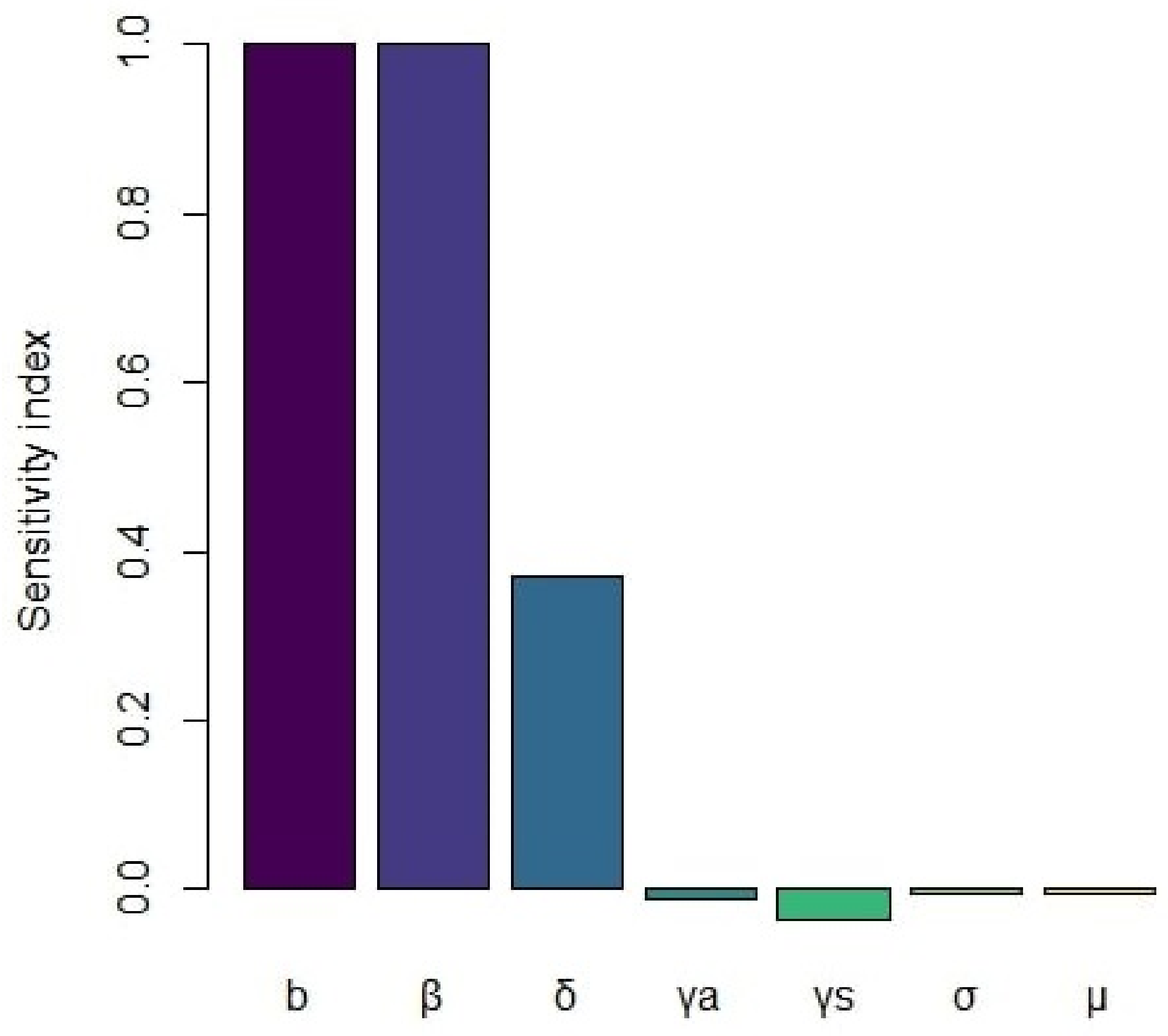
4. Sensitivity of the Basic Reproduction Number

In this section, we conduct a sensitivity analysis of the basic reproduction number ($R_0$) to better understand the influence of each parameter on the transmission of COVID-19, which is directly related to this basic reproduction number. In our case, the key parameters b, $\beta$, ${\gamma }_a$, ${\gamma }_s$, $\delta$, $\sigma$, and $\mu$ are presented in the Table 2 below.

Table 2. Values of the model parameters.

Parameter	Value	Source
b	0.05	Assumed
$\beta$	0.024	Assumed
$\alpha$	0.9	Assumed
$\delta$	0.7	[46]
${\gamma }_a$	0.25	Assumed
${\gamma }_s$	0.14	Assumed
$\sigma$	0.023	Assumed
$\mu$	0.01	Assumed

By calculating the sensitivity index for each of these parameters, we can identify those that have a significant impact on the threshold ($R_0$). More specifically, these indices can be either positive or negative. A positive index indicates that the value of $R_0$ will increase with an increase in the corresponding parameter, while a negative index indicates that $R_0$ will decrease as the parameter increases. We characterize the normalized sensitivity index of a parameter ($\theta$) as ${\Psi }_{\theta ,R_0}$, which is defined as follows:

$$\begin{array}{c}\hfill {\Psi }_{\theta ,R_0}={\displaystyle \frac{\partial R_0}{\partial \theta }}\times {\displaystyle \frac{\theta }{R_0}}.\end{array}$$

Below, we present the normalized sensitivity indices for the parameters calculated using the parameter values from Table 2.

$${\Psi }_{b,R_0}=1,{\Psi }_{\beta ,R_0}=1,{\Psi }_{\delta ,R_0}={\displaystyle \frac{h_a-h_s}{\delta h_a+(1-\delta )h_s}},$$

$${\Psi }_{{\gamma }_a,R_0}=-{\displaystyle \frac{(1-\delta ){\gamma }_a{h}_s}{h_a(\delta h_a+(1-\delta )h_s)}},{\Psi }_{{\gamma }_s,R_0}=-{\displaystyle \frac{\delta {\gamma }_s{h}_a}{h_s(\delta h_a+(1-\delta )h_s)}},$$

$${\Psi }_{\sigma ,R_0}=-{\displaystyle \frac{\delta \sigma h_a}{h_s(\delta h_a+(1-\delta )h_s)}},\mathrm{a}\mathrm{n}\mathrm{d}{\Psi }_{\mu ,R_0}=-{\displaystyle \frac{(1-\delta )(2\mu +{\gamma }_a)h_s^2+\delta (2\mu +\sigma +{\gamma }_s)h_a^2}{h_a{h}_s(\delta h_a+(1-\delta )h_s)}}.$$

Based on the information from Table 2, the sensitivity indices calculated in Table 3 and are represented in Figure 2. This highlights that the parameters influencing $R_0$ can be categorized into the following two groups based on their effects: those that positively increase $R_0$ and those that reduce it. The parameters b, $\beta$, and $\delta$ have a positive impact on $R_0$, meaning that an increase in these parameters results in a corresponding increase in $R_0$. For instance, a 100% increase in either b or $\beta$ leads to an equivalent 100% increase in $R_0$, while a 100% increase in $\delta$ only induces 30% growth in $R_0$. Conversely, there is a negative relationship between $R_0$ and the parameters ${\gamma }_a$, ${\gamma }_s$, $\delta$, and $\mu$. An increase (or decrease) of 100% in any of these parameters results in a reduction (or increase) of $R_0$, ranging from $0.4\%$ to $3.4\%$.

Table 3. Sensitivity indices for $R_0<1$.

Parameter	Sensitivity Index
b	+1
$\beta$	+1
${\gamma }_a$	−0.0116
${\gamma }_s$	−0.0344
$\delta$	+0.372
$\sigma$	−0.005
$\mu$	−0.004

Figure 2. Sensitivity indices of $R_0$ for all parameters of the model.

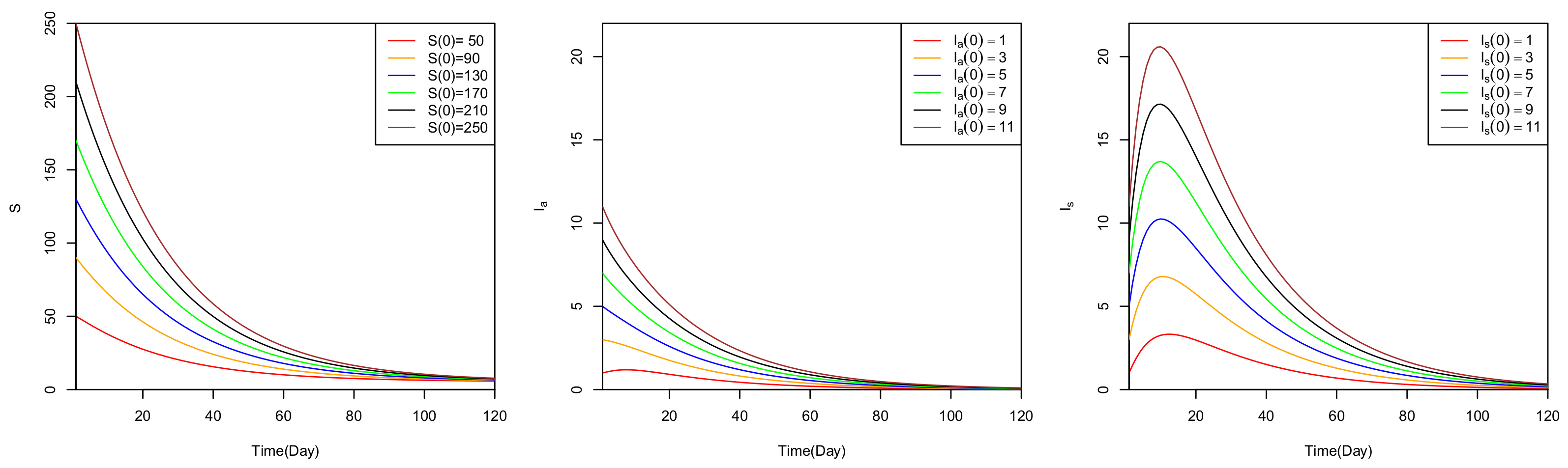
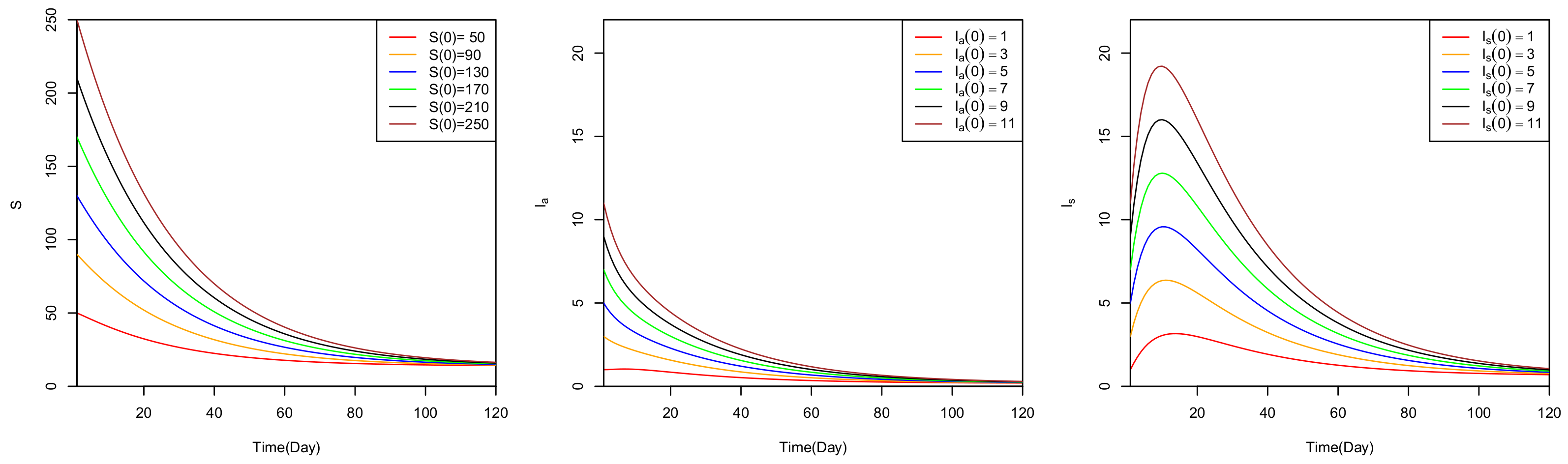
5. Numerical Analysis

Using the parameter values indicated in Table 2, we conduct numerical simulations using R 4.3.0 software, specifically employing the ‘ode()’ function from the deSolve package, which, by default, applies the fourth-order Runge–Kutta method to solve system (3), which represents our model. The primary objective of these simulations is to validate the analytical results from Section 3 through the presentation of graphs illustrating that, when $R_0<1$, the disease-free equilibrium is reached and the infected populations tend toward zero. In contrast, when $R_0>1$, an endemic equilibrium is established, and the disease persists within the population. These simulations also aim to explore the variation of the basic reproduction number ($R_0$) with respect to the main parameters of the model.

Figure 3 presents the behavior of system (3) under different initial conditions when $R_0=0.7<1$, showing that the susceptible population stabilizes at $S_0=5$ as $t\to \infty$, while the asymptomatic and symptomatic populations gradually decrease until they disappear. Consequently, system (3) converges to the disease-free equilibrium $x_{DFE}=(5,0,0)$, as confirmed by Theorem 2. Furthermore, Figure 4 illustrates the behavior of system (3) with different initial conditions when $R_0=3.74>1$, indicating that the populations converge to the endemic equilibrium $x^{*}=(14,0.18,0.65)$) as t approaches infinity, confirming the results of Theorem 4.

Figure 3. Graphs of $S,I_a$, and $I_s$ for $R_0=0.7<1$ with various initial conditions and parameters from Table 2.

Figure 4. Graphs of $S,I_a$, and $I_s$ for $R_0=3.74>1$ and $b=0.3$ with different initial conditions and parameters from the Table 2.

In addition, Figure 5 and Figure 6 examine how the basic reproduction number ($R_0$) changes based on the key parameters of system (3). The Figure 5a,d of specifically highlight the impacts of $\beta$, $\delta$, ${\gamma }_a$, and ${\gamma }_s$ on $R_0$. An increase in $\beta$ or $\delta$ results in a higher $R_0$, thereby accelerating the spread of the virus. Conversely, an increase in ${\gamma }_a$ or ${\gamma }_s$ leads to a reduction in $R_0$, thereby slowing down disease transmission. Figure 6 also presents a 3D visualization of the variations in $R_0$ in relation to the aforementioned parameters.

Figure 5. Variation of $R_0$ with respect to parameters $\beta ,\delta ,{\gamma }_a,{\gamma }_s,\mu$, and $\sigma$. The graphs (a,b) show the increase in $R_0$ as a function of $\beta$ and $\delta$. The graphs (c–f) illustrate the decrease in $R_0$ as a function of the values of ${\gamma }_a$, ${\gamma }_s$, $\mu$, and $\sigma$.

Figure 6. Influence of parameters $\beta$, $\delta$, ${\gamma }_a$, and ${\gamma }_s$ on $R_0$. (a) Sensitivity of $R_0$ to parameters $\beta$ and $\delta$. (b) Sensitivity of $R_0$ to parameters ${\gamma }_a$ and ${\gamma }_s$.

6. Discussion

In this study, we developed a modified SIR model with a nonlinear incidence function, in which the infected populations are divided into the following two classes: asymptomatic and symptomatic individuals. This approach allows for the incorporation of psychological and social behaviors involved in the transmission of COVID-19 [16,43,44,46,47].

The incidence function employed in the proposed model, as opposed to traditional linear incidence models [1,2,3], significantly alters the disease transmission profile. It highlights distinct phases of acceleration and deceleration in the spread of COVID-19 [4,6,10,12,16]. This nonlinear incidence function integrates the complexities of human behavior, although it still relies on simplifying assumptions, such as contact homogeneity (symmetry assumption).

Sensitivity analysis is crucial for identifying the key factors affecting COVID-19’s spread while also emphasizing the dependence of $R_0$ on the various parameters of the model [47]. In summary, this work can assist decision makers in modifying epidemic trends and optimizing public health strategies.

7. Conclusion

In this study, we formulated a mathematical model to examine the dynamics of COVID-19 transmission. In particular, we utilized a modified SIR model with a nonlinear incidence, as detailed in Equation (3). The model distinguishes between the following two types of infected individuals: the asymptomatic and symptomatic populations. It was established that the system consistently yields the following two equilibria: a disease-free equilibrium ($x_{DFE}$) and an endemic equilibrium ($x^{*}$). By utilizing the next-generation matrix method, we determined the basic reproduction number ($R_0$) and explored its dependence on key system parameters in Equation (3). Our analysis demonstrates that when $R_0<1$, the disease-free equilibrium ($x_{DFE}$) is both locally and globally asymptotically stable, and when $R_0>1$, the endemic equilibrium similarly exhibits both local and global asymptotic stability. We conducted a sensitivity analysis to understand the influence of the main parameters of the model on $R_0$. Finally, the analytical results were validated by specific numerical simulations.

References

- Brauer, F.; Castillo-Chavez, C. Mathematical Models in Population Biology and Epidemiology; Springer: New York, NY, USA, 2012. [Google Scholar] [CrossRef]
- Li, H.; Wu, Y. Dynamics of SCIR Modeling for COVID-19 with Immigration. Complexity 2022, 2022. [Google Scholar] [CrossRef]
- Lei, C.; Li, H.; Zhao, Y. Dynamical behavior of a reaction-diffusion SEIR epidemic model with mass action infection mechanism in a heterogeneous environment. Discret. Contin. Dyn. Syst.-B 2024, 29, 3163–3198. [Google Scholar] [CrossRef]
- Shao, P.; Shateyi, S. Stability Analysis of SEIRS Epidemic Model with Nonlinear Incidence Rate Function. Mathematics 2021, 9, 2644. [Google Scholar] [CrossRef]
- Li, T.; Zhang, F.; Liu, H.; Chen, Y. Threshold dynamics of an SIRS model with nonlinear incidence rate and transfer from infectious to susceptible. Appl. Math. Lett. 2017, 70, 52–57. [Google Scholar] [CrossRef]
- Korobeinikov, A.; Maini, P.K. Non-linear incidence and stability of infectious disease models. Math. Med. Biol. J. IMA 2005, 22, 113–128. [Google Scholar] [CrossRef]
- Korobeinikov, A. Global Properties of Infectious Disease Models with Nonlinear Incidence. Bull. Math. Biol. 2007, 69, 1871–1886. [Google Scholar] [CrossRef]
- Korobeinikov, A. Lyapunov Functions and Global Stability for SIR and SIRS Epidemiological Models with Non-Linear Transmission. Bull. Math. Biol. 2006, 68, 615–626. [Google Scholar] [CrossRef]
- Feng, Z.; Thieme, H.R. Endemic Models with Arbitrarily Distributed Periods of Infection I: Fundamental Properties of the Model. SIAM J. Appl. Math. 2000, 61, 803–833. [Google Scholar] [CrossRef]
- Cerón Gómez, M.; Mondragon, E.I.; Molano, P.L. Global stability analysis for a model with carriers and non-linear incidence rate. J. Biol. Dyn. 2020, 14, 409–420. [Google Scholar] [CrossRef]
- Askar, S.; Ghosh, D.; Santra, P.; Elsadany, A.A.; Mahapatra, G. A fractional order SITR mathematical model for forecasting of transmission of COVID-19 of India with lockdown effect. Results Phys. 2021, 24, 104067. [Google Scholar] [CrossRef]
- Alshammari, F.S.; Khan, M.A. Dynamic behaviors of a modified SIR model with nonlinear incidence and recovery rates. Alex. Eng. J. 2021, 60, 2997–3005. [Google Scholar] [CrossRef]
- Ali, A.; Alshammari, F.S.; Islam, S.; Khan, M.A.; Ullah, S. Modeling and analysis of the dynamics of novel coronavirus (COVID-19) with Caputo fractional derivative. Results Phys. 2021, 20, 103669. [Google Scholar] [CrossRef] [PubMed]
- Awais, M.; Alshammari, F.S.; Ullah, S.; Khan, M.A.; Islam, S. Modeling and simulation of the novel coronavirus in Caputo derivative. Results Phys. 2020, 19, 103588. [Google Scholar] [CrossRef]
- Basnarkov, L. SEAIR Epidemic spreading model of COVID-19. Chaos Solitons Fractals 2021, 142, 110394. [Google Scholar] [CrossRef] [PubMed]
- Prem Kumar, R.; Basu, S.; Ghosh, D.; Santra, P.K.; Mahapatra, G.S. Dynamical analysis of novel COVID-19 epidemic model with non-monotonic incidence function. J. Public Aff. 2021, 22, e2754. [Google Scholar] [CrossRef]
- Abbasi, Z.; Zamani, I.; Mehra, A.H.A.; Shafieirad, M.; Ibeas, A. Optimal Control Design of Impulsive SQEIAR Epidemic Models with Application to COVID-19. Chaos Solitons Fractals 2020, 139, 110054. [Google Scholar] [CrossRef]
- Basu, S.; Prem Kumar, R.; Santra, P.; Mahapatra, G.; Elsadany, A. Preventive control strategy on second wave of COVID-19 pandemic model incorporating lock-down effect. Alex. Eng. J. 2022, 61, 7265–7276. [Google Scholar] [CrossRef]
- Chen, T.M.; Rui, J.; Wang, Q.P.; Zhao, Z.Y.; Cui, J.A.; Yin, L. A mathematical model for simulating the phase-based transmissibility of a novel coronavirus. Infect. Dis. Poverty 2020, 9, 24. [Google Scholar] [CrossRef]
- Avila-Ponce de León, U.; Pérez, Á.G.; Avila-Vales, E. An SEIARD epidemic model for COVID-19 in Mexico: Mathematical analysis and state-level forecast. Chaos Solitons Fractals 2020, 140, 110165. [Google Scholar] [CrossRef]
- Engbert, R.; Rabe, M.M.; Kliegl, R.; Reich, S. Sequential Data Assimilation of the Stochastic SEIR Epidemic Model for Regional COVID-19 Dynamics. Bull. Math. Biol. 2020, 83, 1. [Google Scholar] [CrossRef]
- Gralinski, L.E.; Menachery, V.D. Return of the Coronavirus: 2019-nCoV. Viruses 2020, 12, 135. [Google Scholar] [CrossRef] [PubMed]
- Ghosh, D.; Santra, P.K.; Mahapatra, G.S.; Elsonbaty, A.; Elsadany, A.A. A discrete-time epidemic model for the analysis of transmission of COVID19 based upon data of epidemiological parameters. Eur. Phys. J. Spec. Top. 2022, 231, 3461–3470. [Google Scholar] [CrossRef] [PubMed]
- Jiao, S.; Huang, M. An SIHR epidemic model of the COVID-19 with general population-size dependent contact rate. AIMS Math. 2020, 5, 6714–6725. [Google Scholar] [CrossRef]
- Khan, M.A.; Atangana, A. Modeling the dynamics of novel coronavirus (2019-nCov) with fractional derivative. Alex. Eng. J. 2020, 59, 2379–2389. [Google Scholar] [CrossRef]
- Khan, M.A.; Atangana, A.; Alzahrani, E.; Fatmawati. The dynamics of COVID-19 with quarantined and isolation. Adv. Differ. Equations 2020, 2020, 425. [Google Scholar] [CrossRef]
- Kuddus, M.A.; Rahman, A. Analysis of COVID-19 using a modified SLIR model with nonlinear incidence. Results Phys. 2021, 27, 104478. [Google Scholar] [CrossRef]
- Prem Kumar, R.; Santra, P.; Mahapatra, G. Global stability and analysing the sensitivity of parameters of a multiple-susceptible population model of SARS-CoV-2 emphasising vaccination drive. Math. Comput. Simul. 2023, 203, 741–766. [Google Scholar] [CrossRef]
- Kumar, R.P.; Basu, S.; Santra, P.; Ghosh, D.; Mahapatra, G. Optimal control design incorporating vaccination and treatment on six compartment pandemic dynamical system. Results Control Optim. 2022, 7, 100115. [Google Scholar] [CrossRef]
- Richard, Q.; Alizon, S.; Choisy, M.; Sofonea, M.T.; Djidjou-Demasse, R. Age-structured non-pharmaceutical interventions for optimal control of COVID-19 epidemic. PLoS Comput. Biol. 2021, 17, e1008776. [Google Scholar] [CrossRef]
- Ram, V.; Schaposnik, L.P. A modified age-structured SIR model for COVID-19 type viruses. Sci. Rep. 2021, 11. [Google Scholar] [CrossRef]
- Pal, D.; Ghosh, D.; Santra, P.K.; Mahapatra, G.S. Mathematical Analysis of a COVID-19 Epidemic Model by Using Data Driven Epidemiological Parameters of Diseases Spread in India. Biophysics 2022, 67, 231–244. [Google Scholar] [CrossRef] [PubMed]
- Pal, D.; Ghosh, D.; Santra, P.K.; Mahapatra, G.S. Mathematical modeling and analysis of COVID-19 infection spreads in India with restricted optimal treatment on disease incidence. BIOMATH 2021, 10. [Google Scholar] [CrossRef]
- Saldaña, F.; Flores-Arguedas, H.; Camacho-Gutiérrez, J.A.; Barradas, I. Modeling the transmission dynamics and the impact of the control interventions for the COVID-19 epidemic outbreak. Math. Biosci. Eng. 2020, 17, 4165–4183. [Google Scholar] [CrossRef] [PubMed]
- Silva, P.C.; Batista, P.V.; Lima, H.S.; Alves, M.A.; Guimarães, F.G.; Silva, R.C. COVID-ABS: An agent-based model of COVID-19 epidemic to simulate health and economic effects of social distancing interventions. Chaos Solitons Fractals 2020, 139, 110088. [Google Scholar] [CrossRef]
- Xie, Y.; Wang, Z. Transmission dynamics, global stability and control strategies of a modified SIS epidemic model on complex networks with an infective medium. Math. Comput. Simul. 2021, 188, 23–34. [Google Scholar] [CrossRef]
- Yang, C.; Wang, J. A mathematical model for the novel coronavirus epidemic in Wuhan, China. Math. Biosci. Eng. 2020, 17, 2708–2724. [Google Scholar] [CrossRef]
- Day, M. COVID-19: Four fifths of cases are asymptomatic, China figures indicate. BMJ 2020, 369, m1375. [Google Scholar] [CrossRef]
- He, D.; Zhao, S.; Lin, Q.; Zhuang, Z.; Cao, P.; Wang, M.H.; Yang, L. The relative transmissibility of asymptomatic COVID-19 infections among close contacts. Int. J. Infect. Dis. 2020, 94, 145–147. [Google Scholar] [CrossRef]
- Tomochi, M.; Kono, M. A mathematical model for COVID-19 pandemic—SIIR model: Effects of asymptomatic individuals. J. Gen. Fam. Med. 2020, 22, 5–14. [Google Scholar] [CrossRef]
- Ahmed, I.; Modu, G.U.; Yusuf, A.; Kumam, P.; Yusuf, I. A mathematical model of Coronavirus Disease (COVID-19) containing asymptomatic and symptomatic classes. Results Phys. 2021, 21, 103776. [Google Scholar] [CrossRef]
- Kuhl, E. Computational Epidemiology: Data-Driven Modeling of COVID-19; Springer International Publishing: Cham, Switzerland, 2021. [Google Scholar] [CrossRef]
- Ottaviano, S.; Sensi, M.; Sottile, S. Global stability of SAIRS epidemic models. Nonlinear Anal. Real World Appl. 2022, 65, 103501. [Google Scholar] [CrossRef]
- Essak, A.A.; Boukanjime, B. Global stability of an SAIRS epidemic model with vaccinations, transient immunity and treatment. Nonlinear Anal. Real World Appl. 2023, 73, 103887. [Google Scholar] [CrossRef]
- Ying, L.; Tang, X. COVID-19: Is it safe now? Study of asymptomatic infection spread and quantity risk based on SAIR model. Chaos Solitons Fractals X 2021, 6, 100060. [Google Scholar] [CrossRef]
- Mwalili, S.; Kimathi, M.; Ojiambo, V.; Gathungu, D.; Mbogo, R. SEIR model for COVID-19 dynamics incorporating the environment and social distancing. BMC Res. Notes 2020, 13, 352. [Google Scholar] [CrossRef]
- Ma, C.; Li, X.; Zhao, Z.; Liu, F.; Zhang, K.; Wu, A.; Nie, X. Understanding Dynamics of Pandemic Models to Support Predictions of COVID-19 Transmission: Parameter Sensitivity Analysis of SIR-Type Models. IEEE J. Biomed. Health Inform. 2022, 26, 2458–2468. [Google Scholar] [CrossRef]
- Hale, J. Ordinary Differential Equations; Dover Books on Mathematics; Dover Publications: Mineola, NY, USA, 1969; p. 384. [Google Scholar]
- Birkhoff, G.; Rota, G.C. Ordinary Differential Equations, 4th ed.; Wiley: Hoboken, NJ, USA, 1991; p. 416. [Google Scholar]
- Diekmann, O.; Heesterbeek, J.; Metz, J. On the definition and the computation of the basic reproduction ratio R0 in models for infectious diseases in heterogeneous populations. J. Math. Biol. 1990, 28, 365–381. [Google Scholar] [CrossRef]
- van den Driessche, P.; Watmough, J. Reproduction numbers and sub-threshold endemic equilibria for compartmental models of disease transmission. Math. Biosci. 2002, 180, 29–48. [Google Scholar] [CrossRef]
- La Salle, J.P. The Stability of Dynamical Systems; Society for Industrial and Applied Mathematics: Philadelphia, PA, USA, 1976. [Google Scholar] [CrossRef]
- La Salle, J.; Lefschetz, S.; Alverson, R.C. Stability by Liapunov’s Direct Method With Applications. Phys. Today 1962, 15, 59. [Google Scholar] [CrossRef]
Disclaimer/Publisher’s Note: The statements, opinions and data contained in all publications are solely those of the individual author(s) and contributor(s) and not of MDPI and/or the editor(s). MDPI and/or the editor(s) disclaim responsibility for any injury to people or property resulting from any ideas, methods, instructions or products referred to in the content. |
© 2024 by the authors. Licensee MDPI, Basel, Switzerland. This article is an open access article distributed under the terms and conditions of the Creative Commons Attribution (CC BY) license (https://creativecommons.org/licenses/by/4.0/).