Hesitant Bipolar-Valued Intuitionistic Fuzzy Graphs for Identifying the Dominant Person in Social Media Groups

Abstract

This work introduces the notion of a hesitant bipolar-valued intuitionistic fuzzy graph (HBVIFG), which reflects four different characterizations: membership with positive/negative aspects and non-membership with positive/negative aspects, incorporating multi-dimensional alternatives in all of its information. HBVIFG generalizes both HBVFG and BVHFG due to its diversified nature in observing four perspectives along with multiple attributes in a piece of information. Numerous studies, examples, and graphical representations emphasize the concept’s distinctiveness and importance. The following graph theory terms are defined: strong directed HBVIFG, full directed HBVIFG, directed spanning HBVIFSG, directed HBVIFSG, and partial directed hesitant bipolar-valued intuitionistic fuzzy subgraph (HBVIFSG). Examples of operations utilizing two HBVIFGs are Cartesian, direct, lexicographical, and strong products. A scenario is used to generate the mapping of relations, which includes homomorphism, isomorphism, weak isomorphism, and co-weak isomorphism. We describe a directed HBVIFG application that employs an algorithm to determine the most dominant person and self-persistent person in a social system and a comparative study is also provided. The proposed method provides a more detailed framework for assessing the most dominant and self-persistent individual in a social network across multi-level attributes along with positive and negative side membership and non-membership grades in each element of a network.

1. Introduction

1.1. Bipolar-Valued Hesitant Fuzzy Set

Klir and Yuan [1] established fuzzy set theory, which resolves uncertainty caused by poorly defined class boundaries. The membership function, an extension of the characteristic function, denotes a fuzzy set in which each element is characterized by a membership degree taken from $[0,1]$. Since its conception, fuzzy set theory has become a prominent research subject across several fields, resulting in countless developments. Zhang [2] created bipolar-valued fuzzy sets, which are fuzzy sets with membership values spanning from −1 to 1. In these sets, a membership degree of 0 implies irrelevance to the provided context; (0, 1] shows pleasure with certain qualities; and [−1, 0] suggests partial satisfaction with some of the context’s inverse attributes. This expansion handles the satisfaction levels of elements for a situation’s relevant and counter characteristics, but real-world concerns remain a barrier. Bipolar-valued hesitant fuzzy sets were presented by Mandal and Ranadive [3] to solve issues in bipolar membership degrees with reluctance. To manage ambiguous and multidimensional data in decision-making, Mahmood et al. [4] investigated complex hesitant fuzzy sets (CHFS), an extension of hesitant fuzzy sets (HFS), and complex fuzzy sets (CFS). Bao Qing Hu talked about three-way judgments utilizing bipolar-valued fuzzy sets, whereas Ubaid Ur Rehman et al. [5] explored the idea of complex dual hesitant fuzzy sets (CDHFS) and described their working rules. In [6], Hu’s work, partial ordering on truth values in bipolar-valued fuzzy sets and three-way decision spaces are examined, decision evaluation functions based on these sets are presented, and a credit card applicant evaluation example is used to highlight the advantages of semi- or quasi-three-way decision evaluation functions.

1.2. Bipolar Hesitant Fuzzy Graphs

Kauffmann [7] laid the groundwork for fuzzy graph theory by introducing fuzzy graphs utilizing fuzzy relations on fuzzy sets. By establishing a number of fuzzy parameters that are comparable to conventional graph parameters, Rosenfeld [8] expanded on this idea and formalized the idea of a fuzzy graph. Yeh and Bang [9] expounded on several facets of fuzzy graph interconnections at the same time. Due to its many uses and inherent difficulties, fuzzy graph theory has grown in importance within the field of mathematics. Examples of these issues include data extraction, social interaction, clustering, and decision-making. It is essential to the modeling, maintenance, and application of many real-world traffic management and networking concerns. Several fuzzy graph properties allow for the precise assessment of network efficacy and efficiency. Many scholars have made significant contributions to the theoretical development of fuzzy graph theory since Rosenfeld’s groundbreaking work. Strong arcs and fuzzy end nodes were established by [10,11] Bhutani, Rosenfeld, and Bhattacharya, who also provided insights into fuzzy graphs [12]. Mordeson and Nair [13,14] studied fuzzy graphs with arc disjoint states, cycles, and co-cycles. A fuzzy graph matching technique was presented by Gross et al. [15] as a means of intelligent analysis to preserve situational awareness. A practical technique was used by Fan et al. [16] to clarify the notion of bipartite fuzzy graphs, and several forms of photo fuzzy graphs have been discussed [17,18]. Based on the bipolarity of fuzzy sets, Rajeshwari et al. [19] established the idea of bipolar fuzzy sets. The literature provides a thorough explanation of the characteristics, functions, and uses of bipolar fuzzy sets and bipolar fuzzy relations in a variety of academic fields [20]. Bipolar fuzzy graphs (BFGs), isomorphism on BFGs, complement, and its applications were introduced by Akram [21,22]. It is also recorded how fuzzy soft and bipolar fuzzy soft graphs were introduced and how they were used in wireless internet applications [23,24]. Poulik and Ghorai [25] investigated the possible applications of geodesic range and various node kinds in BFGs. Subsequent research describes various degrees and indices of bipolar fuzzy graphs and their ramifications [26,27].

1.3. Bipolar Intuitionistic Fuzzy Graph

The notion of intuitionistic fuzzy sets (IFS), which take into account the belongingness, non-belongingness, and hesitation degrees of items, was first introduced by Atanassov [28]. To investigate intuitionistic fuzzy interactions inside IFS, he expanded this idea using intuitionistic fuzzy graphs (IFG). Since the uncertain information need not rely on membership values alone, there is a possibility of existence of non-membership values. By considering this, Davvaz et al. [29] used IFG of $n^{th}$ type to analyze social networks as it facilitates the membership and non-membership values can be selected from anywhere in [0, 1] regardless of any condition. If an effective edge connects two vertices in an IFG, then those vertices are said to dominate one another [30]. The notions of covering and matching in fuzzy networks with strong edges instead of effective ones were first presented by Manjusha and Sunitha [31]. These ideas were expanded upon by Sahoo et al. [32] to solve problems in intuitionistic fuzzy settings. These concepts were extended to bipolar intuitionistic fuzzy graphs (BIFG) by [33] Deva Nithyanandham et al. They established concepts of dominance, coverage, and matching with effective edges and suggested solutions for cases where effective edges are absent. As an extension of competition graphs, Deva and Felix proposed bipolar intuitionistic fuzzy competition graphs [34]. A fuzzy graph designed for ease of use in industrial water waste applications was proposed by [35] Kaviyarasu et al. For further study, readers can refer to [36,37,38,39].

1.4. Limitations of the Existing Study

The limitations of the existing approaches include:

• A lack of addressing multiple attributes simultaneously from uncertain or imprecise data in the real world.
• The study of relations in a real-world problem that either contains both positive and negative side information along with multi-dimensional alternatives are not discussed effectively.

1.5. Novelty and Contribution

To overcome the above challenges, we create the notion of HBVIFG (hesitant bipolar-valued intuitionistic fuzzy graph) in this paper. We handle a variety of challenges and enhance decision-making by taking on real-world problems containing several bipolar-valued hesitant membership and non-membership grades. The novelty of our work includes:

• The concept HBVIFS, satisfactory and non-satisfactory values of HBVIFSs, score-based intersection of HBVIFEs, and directed HBVIFG are newly defined along with their brief examples. A flowchart is also given for the construction of HBVIFG. Furthermore, directed HBVIFSG and partial, strong, and complete directed HBVIFGs are also introduced.
• We studied basic operations such as the Cartesian product, the strong product, and the union of two HBVIFGs, as well as homomorphism, isomorphism, weak isomorphism, and co-weak isomorphism in HBVIFGs.
• As an application, we investigate a WhatsApp network via HBVIFG. The dominant and influence index is utilized to find the most dominant and self-persistent person in a WhatsApp network.

We investigate basic operations such as the Cartesian product, the strong product, and the union of two HBVIFGs, as well as homomorphism, isomorphism, weak isomorphism, and co-weak isomorphism in these networks.

The contribution of our study is as follows:

• BIFG is very much useful in addressing both belongingness and non-belongingness of the information along with positive and negative side aspects. However, it cannot efficiently solve the real-world problems that contain multi-dimensional alternatives in each of its pieces of information. To handle these kind of problems, a hesitant fuzzy set is incorporated with BIFG.
• HBVIFG is effective for handling decision-making problems as it observes the positive aspect/negative aspect/belongingness/non-belongingness of each data point in a more detailed manner which in turn helps to find a possible solution.

The structure of the paper is as follows: In Section 2, HBVFSs and its graph theoretical concepts are briefly reviewed. Section 3: Standard operational laws and propositions, as well as the notion and presentation of HBVIFGs. Section 4: Different types of products and homomorphic and isomorphic mapping relations are discussed. Section 5: Using HBVIFGs, a novel algorithmic technique is developed, and a numerical example is shown to find the most significant person. A comparative study is presented to illustrate the effectiveness of our proposed model. Section 6: Conclusion.

2. Preliminaries

This section covers the major implications of hesitant bipolar valued fuzzy set along with its suitable instances.

Definition 1. 

Let $U^{*}$ be a reference set. A bipolar-valued hesitant fuzzy set (BVHFS) $R^{*}$ on $U^{*}$ is defined as $R^{*}=\left\{\langle u^{*},{\vartheta }^{R^{*}}\left(u^{*}\right)\rangle \right|u^{*}\in U^{*}\}$. Here, ${\vartheta }^{R^{*}}\left(u^{*}\right)$ contains the values in $[0,1]\times [-1,0]$ and represents the bipolar-valued membership degrees of $u^{*}\in U^{*}$ to $R^{*}$ where ${\vartheta }^{R^{*}}\left(u^{*}\right)=\{\psi =({\psi }^{+},{\psi }^{-})|\psi \in {\vartheta }^{R^{*}}\}$ such that ${\psi }^{+}\in [0,1]$ and ${\psi }^{-}\in [-1,0]$. The element ${\vartheta }^{R^{*}}\left(u^{*}\right)$ is the BVHF element (BVHFE) of $R^{*}$.

Definition 2. 

Let ${\vartheta }^{R^{*}}\left(u^{*}\right)$ be BVHFE. The score function is defined as

$$\delta \left({\vartheta }^{R^{*}}\left(u^{*}\right)\right)={\displaystyle \frac{1}{l}}\sum _{i=1}^l\delta \left({\psi }_i\right)$$

where l is the number of bipolar values in ${\vartheta }^{R^{*}}\left(u^{*}\right)$ and ${\psi }_i$ is an element of ${\vartheta }^{R^{*}}\left(u^{*}\right)$.

Example 1. 

Let $U^{*}=\{u_1^{*},u_2^{*},u_3^{*}\}$ be a reference set where ${\vartheta }^{R^{*}}\left(u_1^{*}\right)=\{\{0.5,-0.6\},\{0.2,-0.4\}\}$, and ${\vartheta }^{R^{*}}\left(u_2^{*}\right)=\{\{0.4,-0.3\},\{0.6,-0.5\},\{0.2,-0.4\}\}$. ${\vartheta }^{R^{*}}\left(u_3^{*}\right)=\{\{0.5,-0.8\},\{0.3,-0.2\}\}$ denotes the BVHF membership values of $u_i^{*},i=1,2,3$ to the set $R^{*}$. Then, $R^{*},{\mathcal{E}}^{*}$ is defined as $R^{*}=\{\langle u_1^{*},(\{0.5,-0.6\},\{0.2,-0.4\})\rangle ,\langle u_2^{*},(\{0.4,-0.3\},\{0.6,-0.5\},\{0.2,-0.4\})\rangle ;\langle u_3^{*},(\{0.5,-0.8\},\{0.3,-0.2\})\rangle \}$ is the BVHFS on $R^{*}$.

Definition 3. 

Let ${\vartheta }^{R^{*}}\left(u^{*}\right)$ and ${\vartheta }^{S^{*}}\left(u^{*}\right)$ be the two BVHFEs of $R^{*},S^{*}$. Then, their score-based intersection is defined as

$$({\vartheta }^{R^{*}}\left(u^{*}\right)\cap {\vartheta }^{S^{*}}\left(u^{*}\right))=\left\{\begin{array}{c}{\vartheta }^{R^{*}}\left(u^{*}\right),\delta \left({\vartheta }^{R^{*}}\left(u^{*}\right)\right)\le \delta \left({\vartheta }^{S^{*}}\left(u^{*}\right)\right)\hfill \\ {\vartheta }^{S^{*}}\left(u^{*}\right),\delta \left({\vartheta }^{S^{*}}\left(u^{*}\right)\right)\le \delta \left({\vartheta }^{R^{*}}\left(u^{*}\right)\right)\hfill \\ {\vartheta }^{R^{*}}\left(u^{*}\right)or{\vartheta }^{S^{*}}\left(u^{*}\right),\delta \left({\vartheta }^{R^{*}}\left(u^{*}\right)\right)=\delta \left({\vartheta }^{S^{*}}\left(u^{*}\right)\right)\hfill \end{array}\right.$$

Definition 4. 

Let $G=(V,E)$ be a graph. A BVHF graph (BVHFG) with V as a reference set $G^{*}=(R^{*},{\mathcal{E}}^{*})$ where $R^{*}$ and ${\mathcal{E}}^{*}$ are BVHFSs in V and $V^2$, respectively, which is characterized by membership function $R^{*}:V\to P([0,1]\times [-1,0])$ and ${\mathcal{E}}^{*}:V^2\to P([0,1]\times [-1,0])$ with the condition $\delta \left({\vartheta }^{{\mathcal{E}}^{*}}(u_1^{*},u_2^{*})\right)\le min\{\delta \left({\vartheta }^{R^{*}}\left(u_1^{*}\right)\right),\delta \left({\vartheta }^{R^{*}}\left(u_2^{*}\right)\right)\}$, $\forall (u_1^{*},u_2^{*})\in V^2$, and $\delta \left({\vartheta }^{{\mathcal{E}}^{*}}(u_1^{*},u_2^{*})\right)=0$, $\forall (u_1^{*},u_2^{*})\in (V^2-{\mathcal{E}}^{*})$.

Example 2. 

Let $V=\{u_1^{*},u_2^{*},u_3^{*}\}$ and $E=\{(u_1^{*},u_2^{*}),(u_2^{*},u_3^{*}),(u_3^{*},u_1^{*})\}$. The BVHFSs $R^{*},{\mathcal{E}}^{*}$ is defined as $R^{*}=\{\langle u_1^{*},(\{0.2,-0.7\},\{0.4,-0.6\})\rangle ,\langle u_2^{*},(\{0.5,-0.3\},\{0.7,-0.4\},\{0.8,-0.1\})\rangle ,$$\langle u_3^{*},(\{0.3,-0.8\},\{0.5,-0.6\})\rangle \}$, and $\mathcal{E}=\{\langle (u_1^{*},u_2^{*}),(\{0.2,-0.5\},\{0.6,-0.3\})\rangle ,\langle (u_2^{*},u_3^{*}),$$(\{0.4,-0.3\},\{0.6,-0.2\})\rangle ,\langle (u_3^{*},u_1^{*}),(\{0.3,-0.5\},\{0.2,-0.7\})\rangle \}$. Here, $\delta \left({\vartheta }^{R^{*}}\left(u_1^{*}\right)\right)=0.475$, $\delta \left({\vartheta }^{R^{*}}\left(u_2^{*}\right)\right)=0.467$, $\delta \left({\vartheta }^{R^{*}}\left(u_3^{*}\right)\right)=0.55$, $\delta ({\vartheta }^{{\mathcal{E}}^{*}}\left((u_1^{*},u_2^{*})\right)=0.4$, $\delta ({\vartheta }^{{\mathcal{E}}^{*}}\left((u_2^{*},u_3^{*})\right)=0.375$, and $\delta ({\vartheta }^{{\mathcal{E}}^{*}}\left((u_3^{*},u_1^{*})\right)=0.425$.

From the above calculations, it is observed that $G^{*}$ is a BVHFG of $G=(V,E)$ and it is represented in Figure 1.

To identify the dominant and self-persistent person in a WhatsApp network, the values related to membership values (positive/negative) and non-membership values (positive/negative) have to be considered. With this observation, we developed a WhatsApp network as an HBVIFG model. The fundamental ideas of HBVFS, HBVFG, and their related concepts are presented here. These concepts are shifted to HBVIFS, HBVIFG, and their related extensions.

Definition 5. 

Let $U^{\prime }$ be a reference set. A hesitant bipolar valued fuzzy set (HBVFS) $R^{\prime }$ on $U^{\prime }$ is defined as $R^{\prime }=\left\{\langle u^{\prime },{\vartheta }^{R^{\prime }+}\left(u^{\prime }\right),{\vartheta }^{R^{\prime }-}\left(u^{\prime }\right)\rangle \right|u^{\prime }\in U^{\prime }\}$ where ${\vartheta }^{R^{\prime }+}\left(u^{\prime }\right):U^{\prime }\to [0,1]$ and ${\vartheta }^{R^{\prime }-}\left(u^{\prime }\right):U^{\prime }\to [-1,0]$ are called hesitant fuzzy positive and negative elements to the set $R^{\prime }$. ${\vartheta }^{R^{\prime }}\left(u^{\prime }\right)=({\vartheta }^{R^{\prime }+}\left(u^{\prime }\right),{\vartheta }^{R^{\prime }-}\left(u^{\prime }\right))$ is called the hesitant bipolar-valued fuzzy element (HBVFE) to the set $R^{\prime }$. The set of all HBVFSs on $R^{\prime }$ is denoted by ${ϝ}^{\prime }\left(U^{\prime }\right)$. The algebraic sum between two HBVFEs ${\vartheta }^{R^{\prime }}\left(u^{\prime }\right)=({\vartheta }^{R^{\prime }+}\left(u^{\prime }\right),{\vartheta }^{R^{\prime }-}\left(u^{\prime }\right))$ and ${\vartheta }^{S^{\prime }}\left(u^{\prime }\right)=({\vartheta }^{S^{\prime }+}\left(u^{\prime }\right),{\vartheta }^{S^{\prime }-}\left(u^{\prime }\right))$ of $R^{\prime },S^{\prime }\in {ϝ}^{\prime }\left(U^{\prime }\right)$ is defined as follows:

$$\begin{array}{cc}\hfill {\vartheta }^{R^{\prime }}\oplus {\vartheta }^{S^{\prime }}& =(\bigcup _{{\psi }_1^{+}\in {\vartheta }^{R^{\prime }+},{\psi }_2^{+}\in {\vartheta }^{S^{\prime }+}}\{{\psi }_1^{+}+{\psi }_2^{+}-{\psi }_1^{+}{\psi }_2^{+}\},\hfill \\ \hfill & \bigcup _{{\psi }_1^{-}\in {\vartheta }^{R^{\prime }-},{\psi }_2^{-}\in {\vartheta }^{S^{\prime }-}}\{{\psi }_1^{-}+{\psi }_2^{-}+{\psi }_1^{-}{\psi }_2^{-}\})\hfill \end{array}$$

Definition 6. 

Let ${\vartheta }^{R^{\prime }}\left(u^{\prime }\right)=({\vartheta }^{R^{\prime }+}\left(u^{\prime }\right),{\vartheta }^{R^{\prime }-}\left(u^{\prime }\right))$ be HBVFE of $R^{\prime }\in {ϝ}^{\prime }\left(U^{\prime }\right)$. Then,

$$\delta \left({\vartheta }^{R^{\prime }}\left(u^{\prime }\right)\right)={\displaystyle \frac{1}{2}}\left({\displaystyle \frac{{\sum }_{{\psi }^{+}\in {\vartheta }^{R^{\prime }+}\left(u^{\prime }\right)}{\psi }^{+}}{l\left({\vartheta }^{R^{\prime }+}\left(u^{\prime }\right)\right)}}-{\displaystyle \frac{{\sum }_{{\psi }^{-}\in {\vartheta }^{R-}\left(u^{\prime }\right)}{\psi }^{-}}{l\left({\vartheta }^{R^{\prime }-}\left(u^{\prime }\right)\right)}}\right)$$

is called the score function of ${\vartheta }^{R^{\prime }}\left(u^{\prime }\right)$, where $l\left({\vartheta }^{R^{\prime }+}\left(u^{\prime }\right)\right)$ and $l\left({\vartheta }^{R^{\prime }-}\left(u^{\prime }\right)\right)$ are the numbers of the elements in ${\vartheta }^{R^{\prime }+}\left(u^{\prime }\right)$ and ${\vartheta }^{R^{\prime }-}\left(u^{\prime }\right)$ accordingly.

Definition 7. 

Let ${\vartheta }^{R^{\prime }}\left(u^{\prime }\right)=({\vartheta }^{R^{\prime }+}\left(u^{\prime }\right),{\vartheta }^{R^{\prime }-}\left(u^{\prime }\right))$ and ${\vartheta }^{S^{\prime }}\left(u^{\prime }\right)=({\vartheta }^{S^{\prime }+}\left(u^{\prime }\right),{\vartheta }^{S^{\prime }-}\left(u^{\prime }\right))$ be the respective HBVFEs of $R^{\prime },S^{\prime }\in {ϝ}^{\prime }\left(U^{\prime }\right)$. If $\delta \left({\vartheta }^{R^{\prime }}\left(u^{\prime }\right)\right)\le \delta \left({\vartheta }^{S^{\prime }}\left(u^{\prime }\right)\right)$, then HBVFS $R^{\prime }$ is a subset of HBVFS $S^{\prime }$. It is denoted by $R^{\prime }⪯S^{\prime }$.

Example 3. 

Let $U^{\prime }=\{u_1^{\prime },u_2^{\prime },u_3^{\prime }\}$ and $R^{\prime },S^{\prime }\in {ϝ}^{\prime }\left(U^{\prime }\right)$ where $R^{\prime }=\{\langle u_1^{\prime },(\{0.5,0.4,0.2\},\{-0.8,$$-0.3\left\}\right)\rangle ,\langle u_2^{\prime },(\{0.4,0.3\},\{-0.7,-0.8,-0.9\})\rangle ,\langle u_3^{\prime },(\{0.2,0.3,0.5,0.6\},\{-0.2,-0.5,-0.6,-0.7$$\left\}\right)\rangle \}$. $S^{\prime }=\{\langle u_1^{\prime },(\{0.5,0.3,0.7\},\{-0.4,-0.6\})\rangle ,\langle u_2^{\prime },(\{0.5,0.8,0.7,0.6\},\{-0.8,-0.6,-0.7\})\rangle ,$$\langle u_3^{\prime },(\{0.9,0.3\},\{-0.4,-0.5,-0.8\})\rangle \}$.

Here, $\delta \left({\vartheta }^{R^{\prime }}\left(u_1^{\prime }\right)\right)=0.4583$, $\delta \left({\vartheta }^{R^{\prime }}\left(u_2^{\prime }\right)\right)=0.5750$, $\delta \left({\vartheta }^{R^{\prime }}\left(u_3^{\prime }\right)\right)=0.4500$, $\delta \left({\vartheta }^{S^{\prime }}\left(u_1^{\prime }\right)\right)=0.5000$, $\delta \left({\vartheta }^{S^{\prime }}\left(u_2^{\prime }\right)\right)=0.6750$, $\delta \left({\vartheta }^{S^{\prime }}\left(u_3^{\prime }\right)\right)=0.5833$. From Definition 7, we have, $\delta \left({\vartheta }^{R^{\prime }}\left(u_i^{\prime }\right)\right)\le \delta \left({\vartheta }^{S^{\prime }}\left(u_i^{\prime }\right)\right)$, where $i=1,2,3$. Thus, $R^{\prime }⪯S^{\prime }$.

Definition 8. 

Let ${\vartheta }^{R^{\prime }}\left(u^{\prime }\right)=({\vartheta }^{R^{\prime }+}\left(u^{\prime }\right),{\vartheta }^{R^{\prime }-}\left(u^{\prime }\right))$ and ${\vartheta }^{S^{\prime }}\left(u^{\prime }\right)=({\vartheta }^{S^{\prime }+}\left(u^{\prime }\right),{\vartheta }^{S^{\prime }-}\left(u^{\prime }\right))$ be two HBVFEs of $R^{\prime },S^{\prime }\in {ϝ}^{\prime }\left(U^{\prime }\right)$. Then, their score-based intersection is defined as

$$({\vartheta }^{R^{\prime }}\left(u^{\prime }\right)\cap {\vartheta }^{S^{\prime }}\left(u^{\prime }\right))=\left\{\begin{array}{c}{\vartheta }^{R^{\prime }}\left(u^{\prime }\right),\delta \left({\vartheta }^{R^{\prime }}\left(u^{\prime }\right)\right)\le \delta \left({\vartheta }^{S^{\prime }}\left(u^{\prime }\right)\right)\hfill \\ {\vartheta }^{S^{\prime }}\left(u^{\prime }\right),\delta \left({\vartheta }^{S^{\prime }}\left(u^{\prime }\right)\right)\le \delta \left({\vartheta }^{R^{\prime }}\left(u^{\prime }\right)\right)\hfill \\ {\vartheta }^{R^{\prime }}\left(u^{\prime }\right)or{\vartheta }^{S^{\prime }}\left(u^{\prime }\right),\delta \left({\vartheta }^{R^{\prime }}\left(u^{\prime }\right)\right)=\delta \left({\vartheta }^{S^{\prime }}\left(u^{\prime }\right)\right)\hfill \end{array}\right.$$

Definition 9. 

Let ${\vartheta }^{R^{\prime }}\left(u^{\prime }\right)=({\vartheta }^{R^{\prime }+}\left(u^{\prime }\right),{\vartheta }^{R^{\prime }-}\left(u^{\prime }\right))$ and ${\vartheta }^{S^{\prime }}\left(u^{\prime }\right)=({\vartheta }^{S^{\prime }+}\left(u^{\prime }\right),{\vartheta }^{S^{\prime }-}\left(u^{\prime }\right))$ be the respective HBVFEs of $R^{\prime }\in {ϝ}^{\prime }\left(U^{\prime }\right)$ and $S^{\prime }\in {ϝ}^{\prime }\left(V^{\prime }\right)$. Then, the Cartesian product of $R^{\prime }\times S^{\prime }$ is defined as

$$R^{\prime }\times S^{\prime }=\{<(u^{\prime },{\nu }^{\prime }),{\vartheta }^{R^{\prime }}\left(u^{\prime }\right)\cap {\vartheta }^{S^{\prime }}\left({\nu }^{\prime }\right)>|(u^{\prime },{\nu }^{\prime })\in U^{\prime }\times V^{\prime }\}.$$

Example 4. 

Let $U^{\prime }=\{u_1^{\prime },u_2^{\prime },u_3^{\prime }\}$ and $V^{\prime }=\{{\nu }_1^{\prime },{\nu }_2^{\prime }\}$. Let $R^{\prime }\in {ϝ}^{\prime }\left(U^{\prime }\right)$ and $S^{\prime }\in {ϝ}^{\prime }\left(V^{\prime }\right)$ where $R=\{\langle u_1^{\prime },(\{0.4,0.8,0.2\},\{-0.8,-0.3\})\rangle ,\langle u_2^{\prime },(\{0.9,0.6\},\{-0.2,-0.8,-0.9\})\rangle ,\langle u_3^{\prime },\left(\right\{0.2,0.5,$$0.6,0.1\},\{-0.5,-0.6,-0.7\left\}\right)\rangle \}$. $S=\{\langle {\nu }_1^{\prime },(\{0.4,0.7,0.5\},\{-0.6,-0.3\})\rangle ,\langle {\nu }_2^{\prime },\left(\right\{0.7,0.8,0.2,$$0.5\},\{-0.7,-0.6,-0.9\left\}\right)\rangle \}$. Here, $\delta \left({\vartheta }^{R^{\prime }}\left(u_1^{\prime }\right)\right)=0.5083$, $\delta \left({\vartheta }^{R^{\prime }}\left(u_2^{\prime }\right)\right)=0.6917$, $\delta \left({\vartheta }^{R^{\prime }}\left(u_3^{\prime }\right)\right)=0.4750$, $\delta \left({\vartheta }^{S^{\prime }}\left({\nu }_1^{\prime }\right)\right)=0.4917$, $\delta \left({\vartheta }^{S^{\prime }}\left({\nu }_2^{\prime }\right)\right)=0.6417$.

Then, $R^{\prime }\times S^{\prime }=\{\langle (u_1^{\prime },{\nu }_1^{\prime }),(\{0.4,0.7,0.5\},\{-0.6,-0.3\},)\rangle ,\langle (u_1^{\prime },{\nu }_2^{\prime }),(\{0.4,0.8,0.2\},$$\{-0.8,-0.3\})\rangle ,\langle (u_2^{\prime },{\nu }_1^{\prime }),(\{0.4,0.5,0.7\},\{-0.6,-0.3\})\rangle ,\langle (u_2^{\prime },{\nu }_2^{\prime }),(\{0.5,0.8,0.2,0.7\},\{-0.9,$$-0.7,-0.6\left\}\right)\rangle ,\langle (u_3^{\prime },{\nu }_1^{\prime }),(\{0.5,0.1,0.2,0.6\},\{-0.5,-0.7,-0.6\})\rangle ,\langle (u_3^{\prime },{\nu }_2^{\prime }),(\{0.5,0.1,0.2,0.6\},$$\{-0.5,-0.7,-0.6\})\rangle \}$.

The HBVFR $Q^{\prime }$ can be written as $Q^{\prime }=\{\langle (u_1^{\prime },{\nu }_1^{\prime }),(\{0.5,0.4,0.2,0.7\},\{-0.5,-0.1,-0.2\})\rangle ,$$\langle (u_1^{\prime },{\nu }_2^{\prime }),(\{0.5,0.3,0.2\},\{-0.5,-0.8\})\rangle ,\langle (u_2^{\prime },{\nu }_1^{\prime }),(\{0.3,0.1,0.4,0.8\},\{-0.1,-0.2,-0.4\})\rangle ,$$\langle (u_2^{\prime },{\nu }_2^{\prime }),(\{0.8,0.4\},\{-0.5,-0.7,-0.8\})\rangle ,\langle (u_3^{\prime },{\nu }_1^{\prime }),(\{0.8,0.3,0.2,0.4\},\{-0.1,-0.4,-0.9\})\rangle ,$$\langle (u_3^{\prime },{\nu }_2^{\prime }),(\{0.2,0.8\},\{-0.3,-0.4,-0.2\})\rangle \}$.

All elements in $Q^{\prime }$ satisfy $\delta \left({\vartheta }^{Q^{\prime }}(u_i^{\prime },{\nu }_j^{\prime })\right)\le min\{\delta \left({\vartheta }^{R^{\prime }}\left(u_i^{\prime }\right)\right),\delta \left({\vartheta }^{S^{\prime }}\left({\nu }_j^{\prime }\right)\right)\}$ where $i=1,2,3$ and $j=1,2$. For instance, take $i=1,j=1$, then, $\delta \left({\vartheta }^{Q^{\prime }}(u_1^{\prime },{\nu }_1^{\prime })\right)=0.3583\le min\{\delta \left({\vartheta }^{R^{\prime }}\left(u_1^{\prime }\right)\right),$$\delta \left({\vartheta }^{S^{\prime }}\left({\nu }_1^{\prime }\right)\right)\}$ = 0.4917.

Definition 10. 

A directed HBVF graph of $G=(V,E)$ is a pair Ǧ $=(R^{\prime },{\mathcal{E}}^{\prime })$ where R is an HBVIFS in $V^{\prime }$ whose corresponding HBVFE is ${\vartheta }^{R^{\prime }}=({\vartheta }^{R^{\prime }+},{\vartheta }^{R^{\prime }-})$ and ${\mathcal{E}}^{\prime }$ is an HBVFS in $V\times V$ whose corresponding HBVFE is ${\vartheta }^{{\mathcal{E}}^{\prime }}=({\vartheta }^{{\mathcal{E}}^{\prime }+},{\vartheta }^{{\mathcal{E}}^{\prime }-})$ such that $\delta \left({\vartheta }^{{\mathcal{E}}^{\prime }}(u_1^{\prime },u_2^{\prime })\right)\le min\{\delta \left({\vartheta }^{R^{\prime }}\left(u_1^{\prime }\right)\right),\delta \left({\vartheta }^{R^{\prime }}\left(u_2^{\prime }\right)\right)\}$. $\forall u_1^{\prime },u_2^{\prime }\in V$.

3. Hesitant Bipolar Valued Intuitionistic Fuzzy Graph

In this section, we introduce the basic definitions including hesitant bipolar-valued intuitionistic fuzzy set (HBVIFS), its satisfactory and non-satisfactory value, score-based intersection and relation of HBVIF elements, and directed HBVIF graph along with several appropriate examples.

Definition 11. 

Let U be a reference set. A hesitant bipolar-valued intuitionistic fuzzy set (HBVIFS) R on U is defined as $R=\left\{\langle u,{\vartheta }_t^{R+}\left(u\right),{\vartheta }_t^{R-}\left(u\right),{\vartheta }_f^{R+}\left(u\right),{\vartheta }_f^{R-}\left(u\right)\rangle \right|u\in U\}$ where ${\vartheta }_t^{R+}\left(u\right),{\vartheta }_f^{R+}\left(u\right):U\to [0,1]$ and ${\vartheta }_t^{R-}\left(u\right),{\vartheta }_f^{R-}\left(u\right):U\to [-1,0]$. The functions ${\vartheta }_t^{R+}\left(u\right),{\vartheta }_f^{R+}\left(u\right)$ denote the possible satisfactory (membership) and non-satisfactory (non-membership) degree of an element $u\in U$ whereas ${\vartheta }_t^{R-}\left(u\right),{\vartheta }_f^{R-}\left(u\right)$ denote the the possible satisfactory and non-satisfactory degree of $u\in U$ to the implicit counter property to the set U, respectively. For the sake of simplicity, we use ${\vartheta }^R\left(u\right)=({\vartheta }_t^R\left(u\right),{\vartheta }_f^R\left(u\right))$ where ${\vartheta }_t^R\left(u\right)=({\vartheta }_t^{R+}\left(u\right),{\vartheta }_t^{R-}\left(u\right))$ and ${\vartheta }_f^R\left(u\right)=({\vartheta }_f^{R+}\left(u\right),{\vartheta }_f^{R-}\left(u\right))$ for the hesitant bipolar-valued intuitionistic fuzzy element (HBVIFE). The set of all HBVIFS is denoted by $ϝ\left(U\right)$.

Definition 12. 

Let ${\vartheta }^R\left(u\right)=({\vartheta }_t^R\left(u\right),{\vartheta }_f^R\left(u\right))$ be HBVIFE of $\mathsf{R}\in ϝ\left(U\right)$. The hesitant bipolar-valued intuitionistic fuzzy satisfactory value (HBVIFSV) is defined as

$${\delta }_t\left({\vartheta }_t^R\left(u\right)\right)={\displaystyle \frac{1}{2}}\left({\displaystyle \frac{{\sum }_{{\psi }_t^{+}\in {\vartheta }_t^{R+}\left(u\right)}{\psi }_t^{+}}{l\left({\vartheta }_t^{R+}\left(u\right)\right)}}-{\displaystyle \frac{{\sum }_{{\psi }_t^{-}\in {\vartheta }_t^{R-}\left(u\right)}{\psi }_t^{-}}{l\left({\vartheta }_t^{R-}\left(u\right)\right)}}\right)$$

The hesitant bipolar-valued intuitionistic fuzzy non-satisfactory value (HBVIFNSV) is defined as

$${\delta }_f\left({\vartheta }_f^R\left(u\right)\right)={\displaystyle \frac{1}{2}}\left({\displaystyle \frac{{\sum }_{{\psi }_f^{+}\in {\vartheta }_f^{R+}\left(u\right)}{\psi }_f^{+}}{l\left({\vartheta }_f^{R+}\left(u\right)\right)}}-{\displaystyle \frac{{\sum }_{{\psi }_f^{-}\in {\vartheta }_f^{R-}\left(u\right)}{\psi }_f^{-}}{l\left({\vartheta }_f^{R-}\left(u\right)\right)}}\right)$$

Definition 13. 

Let ${\vartheta }^R\left(u\right)=({\vartheta }_t^R\left(u\right),{\vartheta }_f^R\left(u\right))$ and ${\vartheta }^S\left(u\right)=({\vartheta }_t^S\left(u\right),{\vartheta }_f^S\left(u\right))$ be two HBVIFEs of $R,S\in ϝ\left(U\right)$. If ${\delta }_t\left({\vartheta }_t^R\left(u\right)\right)\le {\delta }_t\left({\vartheta }_t^S\left(u\right)\right)$ and ${\delta }_f\left({\vartheta }_t^R\left(u\right)\right)\ge {\delta }_f\left({\vartheta }_t^S\left(u\right)\right)$, then HBVIFS R is a subset of HBVIFS S. It is denoted by $R⪯S$.

Example 5. 

Let $U=\{u_1,u_2,u_3\}$ and $R,S\in ϝ\left(U\right)$ where $R=\{\langle u_1,(\{0.3,0.4,0.6\},\{-0.4,$$-0.8\},\{0.4,0.7\},\{-0.3,-0.6\})\rangle ,\langle u_2,(\{0.4,0.5\},\{-0.2\},\left\{0.3\right\},\{-0.1,-0.3\})\rangle ,\langle u_3,(\left\{0.2\right\},$$\{-0.3\},\{0.3,0.4\},\{-0.3,-0.8\})\rangle \}$. $S=\{\langle u_1,(\{0.7,0.8\},\{-0.4,-0.6\},\left\{0.1\right\},\{-0.2,-0.4,$$-0.8\left\}\right)\rangle ,\langle u_2,(\{0.2,0.4,0.7\},\{-0.3,-0.5\},\left\{0.1\right\},\{-0.2,-0.4\})\rangle ,\langle u_3,(\{0.3,0.7\},\{-0.5\},$$\{0.2,0.5\},\{-0.1,-0.4\})\rangle \}$.

Here, ${\delta }_t\left({\vartheta }_t^R\left(u_1\right)\right)=0.5167$, ${\delta }_f\left({\vartheta }_f^R\left(u_1\right)\right)=0.5$, ${\delta }_t\left({\vartheta }_t^R\left(u_2\right)\right)=0.325$, ${\delta }_f\left({\vartheta }_f^R\left(u_2\right)\right)=0.25$, ${\delta }_t\left({\vartheta }_t^R\left(u_3\right)\right)=0.25$, ${\delta }_f\left({\vartheta }_f^R\left(u_3\right)\right)=0.45$, ${\delta }_t\left({\vartheta }_t^S\left(u_1\right)\right)=0.625$, ${\delta }_f\left({\vartheta }_f^S\left(u_1\right)\right)=0.2833$, ${\delta }_t\left({\vartheta }_t^S\left(u_2\right)\right)=0.4167$, ${\delta }_f\left({\vartheta }_f^S\left(u_2\right)\right)=0.2$, ${\delta }_t\left({\vartheta }_t^S\left(u_3\right)\right)=0.5$, ${\delta }_f\left({\vartheta }_f^S\left(u_3\right)\right)=0.3$. From Definition 13, we have, ${\delta }_t\left({\vartheta }_t^R\left(u_i\right)\right)\le {\delta }_t\left({\vartheta }_t^S\left(u_i\right)\right)$ and ${\delta }_f\left({\vartheta }_f^R\left(u_i\right)\right)\ge {\delta }_f\left({\vartheta }_f^S\left(u_i\right)\right),$ where $i=1,2,3$. Thus, $R⪯S$.

Definition 14. 

Let ${\vartheta }^R\left(u\right)=({\vartheta }_t^R\left(u\right),{\vartheta }_f^R\left(u\right))$ and ${\vartheta }^S\left(u\right)=({\vartheta }_t^S\left(u\right),{\vartheta }_f^S\left(u\right))$ be two HBVIFEs of $R,S\in ϝ\left(U\right)$. Then, their score-based intersection is defined as

$$({\vartheta }_t^R\left(u\right)\cap {\vartheta }_t^S\left(u\right))=\left\{\begin{array}{c}{\vartheta }_t^R\left(u\right),{\delta }_t\left({\vartheta }_t^R\left(u\right)\right)\le {\delta }_t\left({\vartheta }_t^S\left(u\right)\right)\hfill \\ {\vartheta }_t^S\left(u\right),{\delta }_t\left({\vartheta }_t^S\left(u\right)\right)\le {\delta }_t\left({\vartheta }_t^R\left(u\right)\right)\hfill \\ {\vartheta }_t^R\left(u\right)or{\vartheta }_t^S\left(u\right),{\delta }_t\left({\vartheta }_t^R\left(u\right)\right)={\delta }_t\left({\vartheta }_t^S\left(u\right)\right)\hfill \end{array}\right.$$

$$({\vartheta }_f^R\left(u\right)\cap {\vartheta }_f^S\left(u\right))=\left\{\begin{array}{c}{\vartheta }_f^R\left(u\right),{\delta }_f\left({\vartheta }_f^R\left(u\right)\right)\ge {\delta }_f\left({\vartheta }_f^S\left(u\right)\right)\hfill \\ {\vartheta }_f^S\left(u\right),{\delta }_f\left({\vartheta }_f^S\left(u\right)\right)\ge {\delta }_f\left({\vartheta }_f^R\left(u\right)\right)\hfill \\ {\vartheta }_f^R\left(u\right)or{\vartheta }_f^S\left(u\right),{\delta }_f\left({\vartheta }_f^R\left(u\right)\right)={\delta }_f\left({\vartheta }_f^S\left(u\right)\right)\hfill \end{array}\right.$$

Proposition 1. 

Let ${\vartheta }^R\left(u\right)$ and ${\vartheta }^S\left(u\right)$ be two HBVIFEs of $R,S\in ϝ\left(U\right)$. If $R⪯S$, then ${\delta }_t\left({\vartheta }_t^R\left(u\right)\right)\le {\delta }_t\left({\vartheta }_t^S\left(u\right)\right)$ and ${\delta }_f\left({\vartheta }_f^R\left(u\right)\right)\ge {\delta }_f\left({\vartheta }_f^S\left(u\right)\right)$.

Proposition 2. 

Let ${\vartheta }^R\left(u\right)$ and ${\vartheta }^S\left(u\right)$ be the corresponding HBVIFEs of $R,S\in ϝ\left(U\right)$, respectively, then

• ${\delta }_t({\vartheta }_t^R\left(u\right)\cap {\vartheta }_t^S\left(u\right))=min\{{\delta }_t\left({\vartheta }_t^R\left(u\right)\right),{\delta }_t\left({\vartheta }_t^S\left(u\right)\right)\}$,
• ${\delta }_f({\vartheta }_f^R\left(u\right)\cap {\vartheta }_f^S\left(u\right))=max\{{\delta }_f\left({\vartheta }_f^R\left(u\right)\right),{\delta }_f\left({\vartheta }_f^S\left(u\right)\right)\}$.

Definition 15. 

Let ${\vartheta }^R=({\vartheta }_t^R,{\vartheta }_f^R)$ and ${\vartheta }^S=({\vartheta }_t^S,{\vartheta }_f^S)$ be two HBVIFEs of $R\in ϝ\left(U\right)$ and $S\in ϝ\left(V\right)$, respectively. Then, the Cartesian product of $R\times S$ is defined as

$$R\times S=\{<(u,\nu ),{\vartheta }_t^R\left(u\right)\cap {\vartheta }_t^S\left(\nu \right),{\vartheta }_f^R\left(u\right)\cap {\vartheta }_f^S\left(\nu \right)>|(u,\nu )\in U\times V\}.$$

Definition 16. 

Let ${\vartheta }^R$ and ${\vartheta }^S$ be two HBVIFEs of $R\in ϝ\left(U\right)$ and $S\in ϝ\left(V\right)$, respectively. Then, the hesitant bipolar-valued intuitionistic fuzzy relation (HBVIFR) Q from HBVIFS R into HBVIFS S is an HBVIFS on $R\times S$ such that

• ${\delta }_t\left({\vartheta }_t^Q(u,\nu )\right)\le min\{{\delta }_t\left({\vartheta }_t^R\left(u\right)\right),{\delta }_t\left({\vartheta }_t^S\left(\nu \right)\right)\}$,
• ${\delta }_f\left({\vartheta }_f^Q(u,\nu )\right)\ge max\{{\delta }_f\left({\vartheta }_f^R\left(u\right)\right),{\delta }_f\left({\vartheta }_f^S\left(\nu \right)\right)\}$.

$\forall (u,\nu )\in U\times V$ and ${\vartheta }^Q=({\vartheta }_t^Q,{\vartheta }_f^Q)$ is the corresponding HBVIFE of Q. If $U=V$, then Q is called HBVIFR on U, respectively.

Example 6. 

Let $U=\{u_1,u_2\}$ and $V=\{{\nu }_1,{\nu }_2,{\nu }_3\}$. Let $R\in ϝ\left(U\right)$ and $S\in ϝ\left(V\right)$ where $R=\{\langle u_1,(\{0.2,0.4\},\{-0.3,-0.8\},\{0.1,0.2\},\{-0.1,-0.5\})\rangle ,\langle u_2,(\left\{0.2\right\},\{-0.2,-0.3\},\{0.1,0.3\},$$\{-0.2,-0.5\})\rangle \}$. $S=\{\langle {\nu }_1,(\{0.5,0.8\},\{-0.4,-0.5\},\left\{0.2\right\},\{-0.2,-0.4,-0.8\})\rangle ,\langle {\nu }_2,\left(\right\{0.2,$$0.4,0.7\},\{-0.1,-0.3\},\{0.4,0.5\},\{-0.3,-0.4,-0.5\})\rangle ,\langle {\nu }_3,(\{0.3,0.6\},\{-0.5\},\{0.2,0.4\},$$\{-0.1,-0.3,-0.5\})\rangle \}$.

Here, ${\delta }_t\left({\vartheta }_t^R\left(u_1\right)\right)=0.425$, ${\delta }_f\left({\vartheta }_f^R\left(u_1\right)\right)=0.225$, ${\delta }_t\left({\vartheta }_t^R\left(u_2\right)\right)=0.225$, ${\delta }_f\left({\vartheta }_f^R\left(u_2\right)\right)=0.275$, ${\delta }_t\left({\vartheta }_t^S\left({\nu }_1\right)\right)=0.55$, ${\delta }_f\left({\vartheta }_f^S\left({\nu }_1\right)\right)=0.3334$, ${\delta }_t\left({\vartheta }_t^S\left({\nu }_2\right)\right)=0.3167$, ${\delta }_f\left({\vartheta }_f^S\left({\nu }_2\right)\right)=0.425$, ${\delta }_t\left({\vartheta }_t^S\left({\nu }_3\right)\right)=0.475$, ${\delta }_f\left({\vartheta }_f^S\left({\nu }_3\right)\right)=0.3$.

Then, $R\times S=\{\langle (u_1,{\nu }_1),(\{0.2,0.4\},\{-0.3,-0.8\},\left\{0.2\right\},\{-0.2,-0.4,-0.8\})\rangle ,\langle (u_1,{\nu }_2),$$(\{0.2,0.4,0.7\},\{-0.1,-0.3\},\{0.4,0.5\},\{-0.3,-0.4,-0.5\})\rangle ,\langle (u_1,{\nu }_3),(\{0.2,0.4\},\{-0.3,$$-0.8\},\{0.2,0.4\},\{-0.1,-0.3,-0.5\})\rangle ,\langle (u_2,{\nu }_1),(\left\{0.2\right\},\{-0.2,-0.3\},\left\{0.2\right\},\{-0.2,-0.4,$$-0.8\left\}\right)\rangle ,\langle (u_2,{\nu }_2),(\left\{0.2\right\},\{-0.2,-0.3\},\{0.4,0.5\},\{-0.3,-0.4,-0.5\})\rangle ,\langle (u_2,{\nu }_3),(\left\{0.2\right\},$$\{-0.2,-0.3\},\{0.2,0.4\},\{-0.1,-0.3,-0.5\})\rangle \}$.

The HBVIFR Q can be written as $Q=\{\langle (u_1,{\nu }_1),(\{0.1,0.2,0.4\},\{-0.2,-0.3\},\{0.2,0.3\},$$\{-0.4,-0.5,-0.6,-0.8\})\rangle ,\langle (u_1,{\nu }_2),(\{0.1,0.2,0.4\},\{-0.1,-0.3\},\{0.5,0.7\},\{-0.3,-0.4,$$-0.5\left\}\right)\rangle ,\langle (u_1,{\nu }_3),(\{0.1,0.3\},\{-0.2,-0.6\},\{0.2,0.4,0.6\},\{-0.1,-0.3,-0.7\})\rangle ,\langle (u_2,{\nu }_1),$$(\left\{0.2\right\},\{-0.1,-0.2,-0.3\},\{0.2,0.4\},\{-0.3,-0.5,-0.8\})\rangle ,\langle (u_2,{\nu }_2),(\left\{0.2\right\},\{-0.1,-0.2\},$$\{0.4,0.5\},\{-0.3,-0.4,-0.5,-0.8\})\rangle ,\langle (u_2,{\nu }_3),(\left\{0.1\right\},\{-0.1,-0.3\},\{0.3,0.6\},\{-0.3,-0.8\})\rangle \}$.

All elements in Q satisfy ${\delta }_t\left({\vartheta }_t^Q(u_i,{\nu }_j)\right)\le min\{{\delta }_t\left({\vartheta }_t^R\left(u_i\right)\right),{\delta }_t\left({\vartheta }_t^S\left({\nu }_j\right)\right)\}$ and ${\delta }_f\left({\vartheta }_f^Q(u_i,{\nu }_j)\right)\ge max\{{\delta }_f\left({\vartheta }_f^R\left(u_i\right)\right),{\delta }_f\left({\vartheta }_f^S\left({\nu }_j\right)\right)\}$ where $i=1,2$ and $j=1,2,3$. For instance, take $i=2,j=2$, then, ${\delta }_t\left({\vartheta }_t^Q(u_2,{\nu }_2)\right)=0.125\le min\{{\delta }_t\left({\vartheta }_t^R\left(u_2\right)\right),{\delta }_t\left({\vartheta }_t^S\left({\nu }_2\right)\right)\}$ and ${\delta }_f\left({\vartheta }_f^Q(u_2,{\nu }_2)\right)=0.475\ge max\{{\delta }_f\left({\vartheta }_f^R\left(u_i\right)\right),{\delta }_f\left({\vartheta }_f^S\left({\nu }_j\right)\right)\}$.

Definition 17. 

A directed HBVIFG of $G=(V,E)$ is a pair Ǧ $=(R,\mathcal{E})$ where R is an HBVIFS in V whose corresponding HBVIFE is ${\vartheta }^R=({\vartheta }_t^R,{\vartheta }_f^R)$ and $\mathcal{E}$ is an HBVIFS in $V\times V$ whose corresponding HBVIFE is ${\vartheta }^{\mathcal{E}}=\left({\vartheta }_t^{\mathcal{E}}{\vartheta }_f^{\mathcal{E}}\right)$ such that

• ${\delta }_t\left({\vartheta }_t^{\mathcal{E}}(u_1,u_2)\right)\le min\{{\delta }_t\left({\vartheta }_t^R\left(u_1\right)\right),{\delta }_t\left({\vartheta }_t^R\left(u_2\right)\right)\}$,
• ${\delta }_f\left({\vartheta }_f^{\mathcal{E}}(u_1,u_2)\right)\ge max\{{\delta }_f\left({\vartheta }_f^R\left(u_1\right)\right),{\delta }_f\left({\vartheta }_f^R\left(u_2\right)\right)\}$.

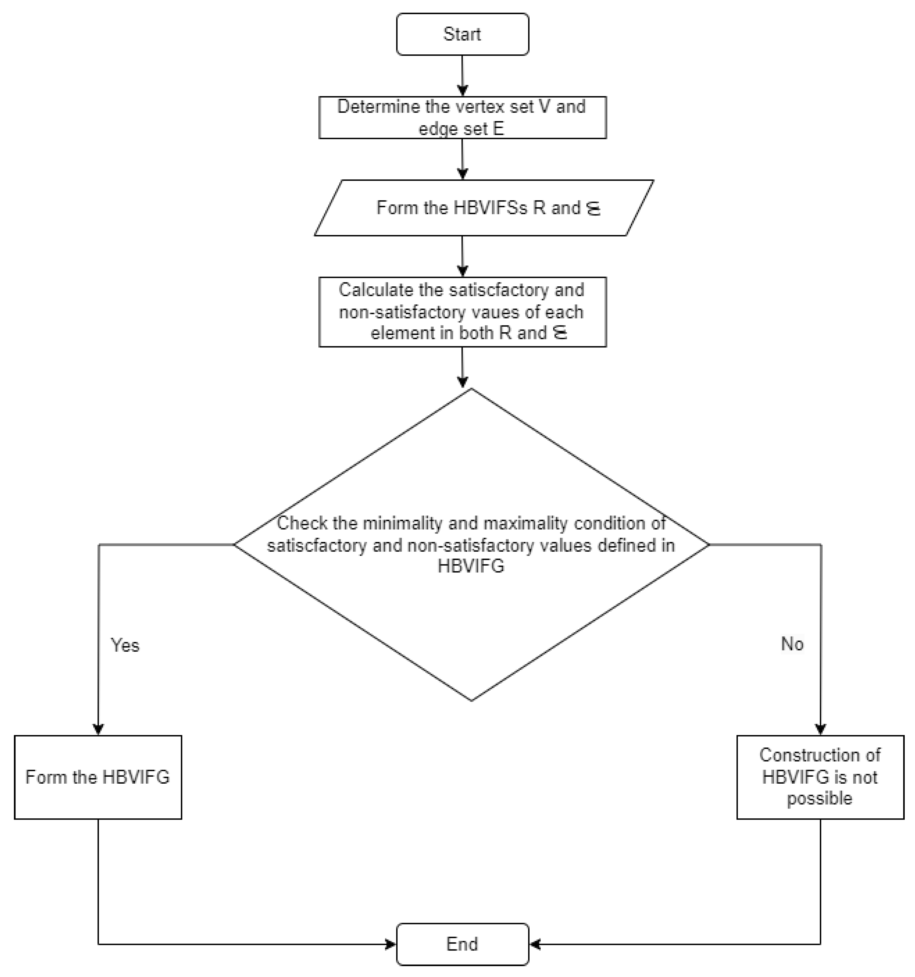
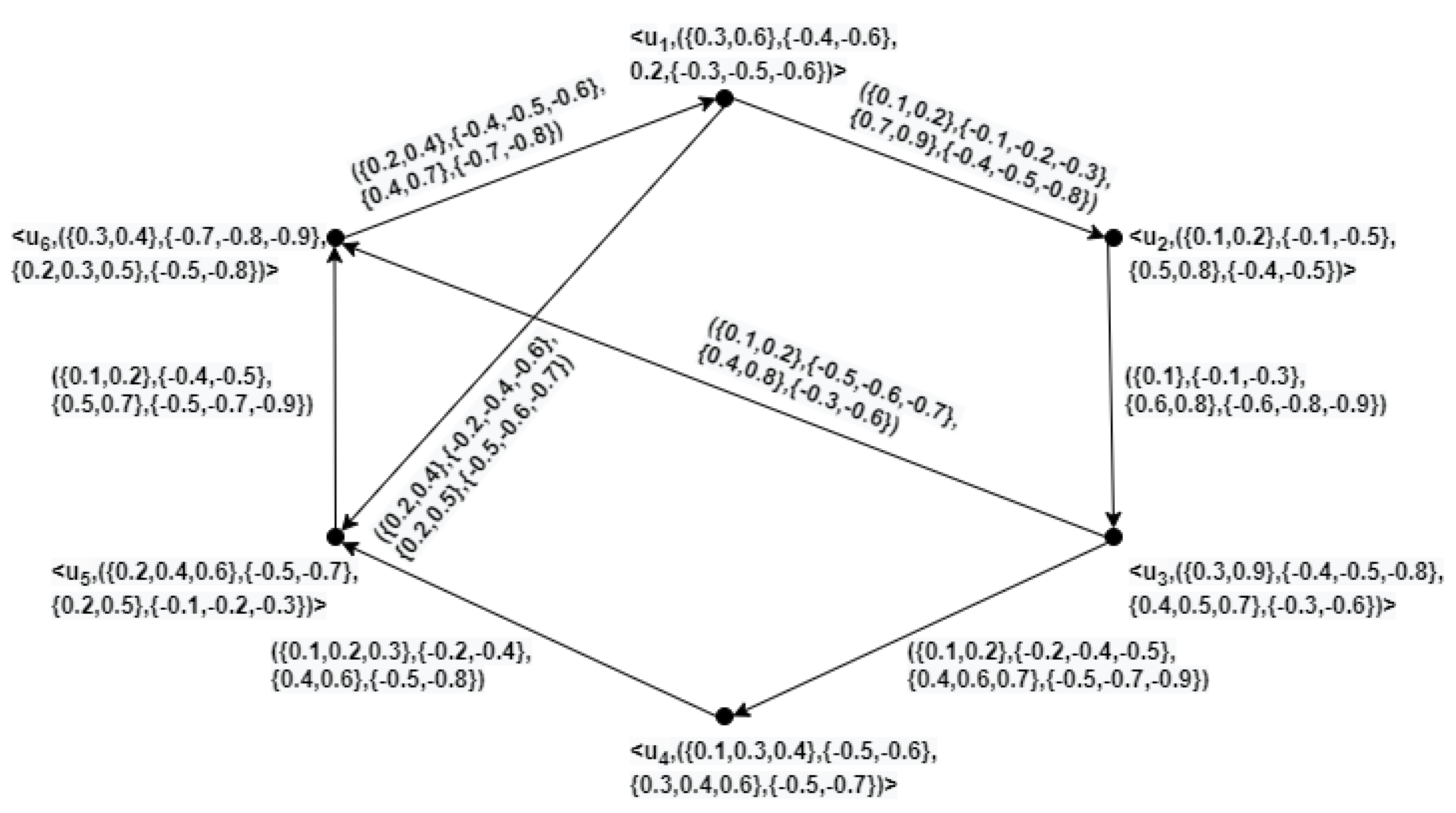
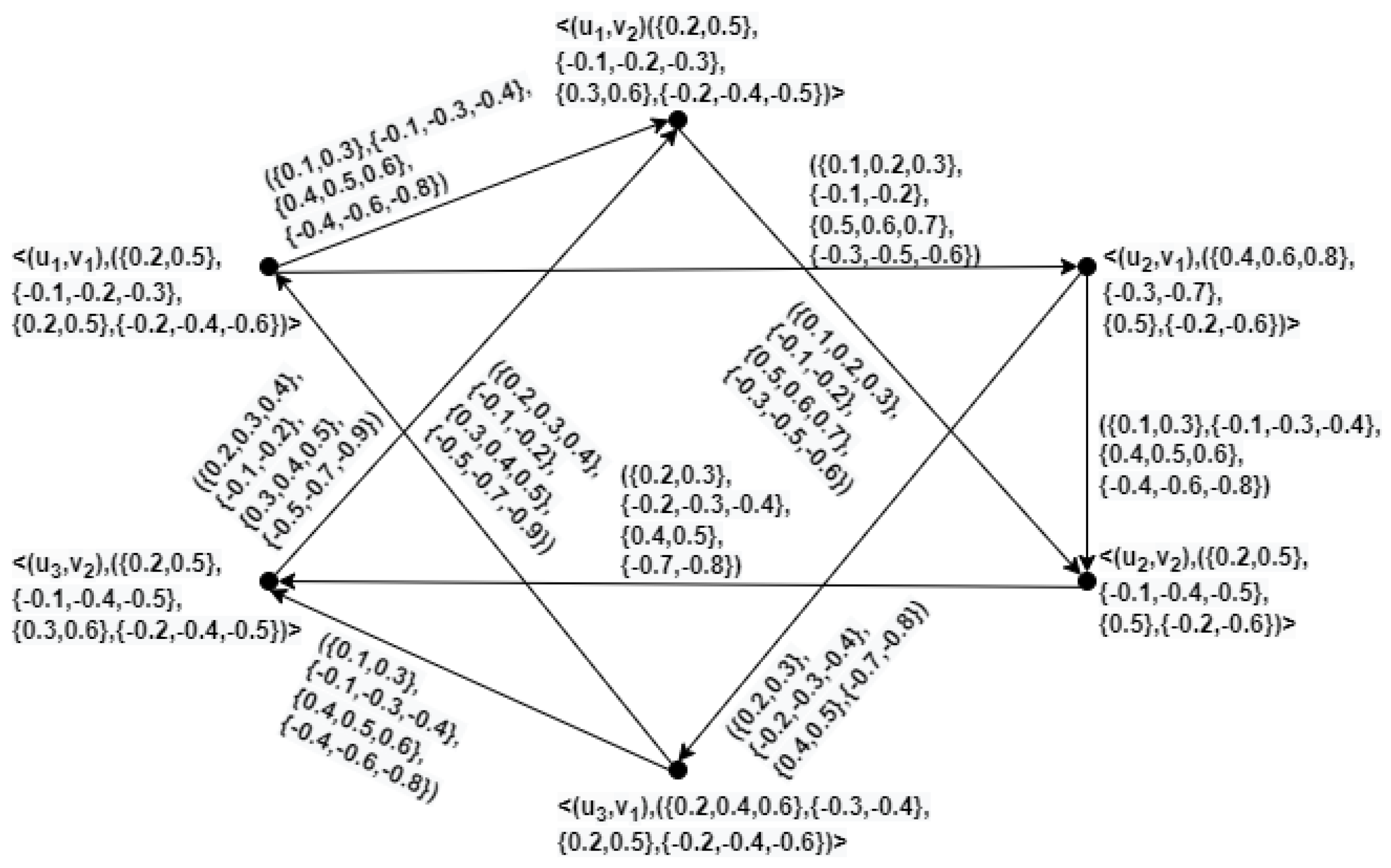
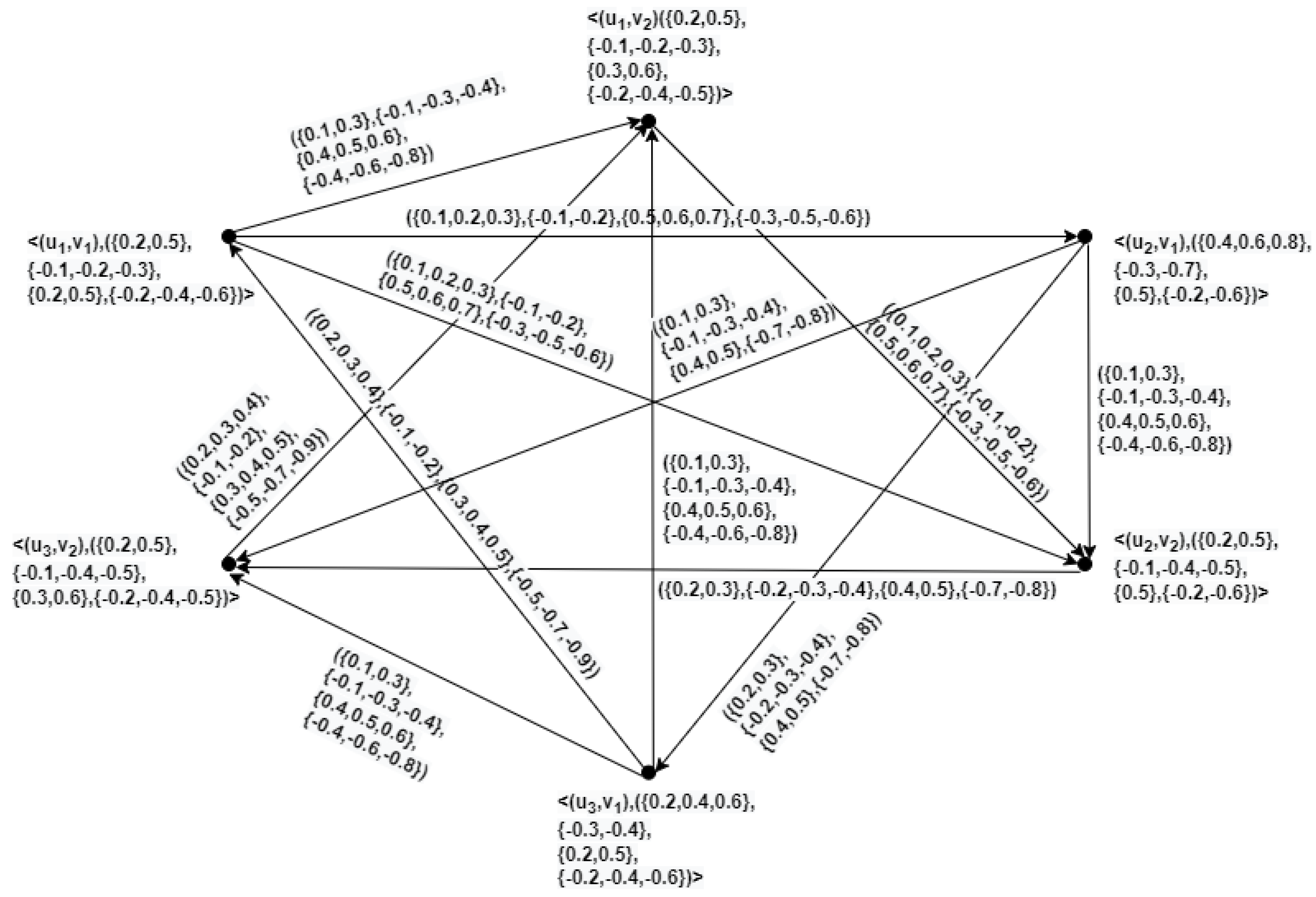
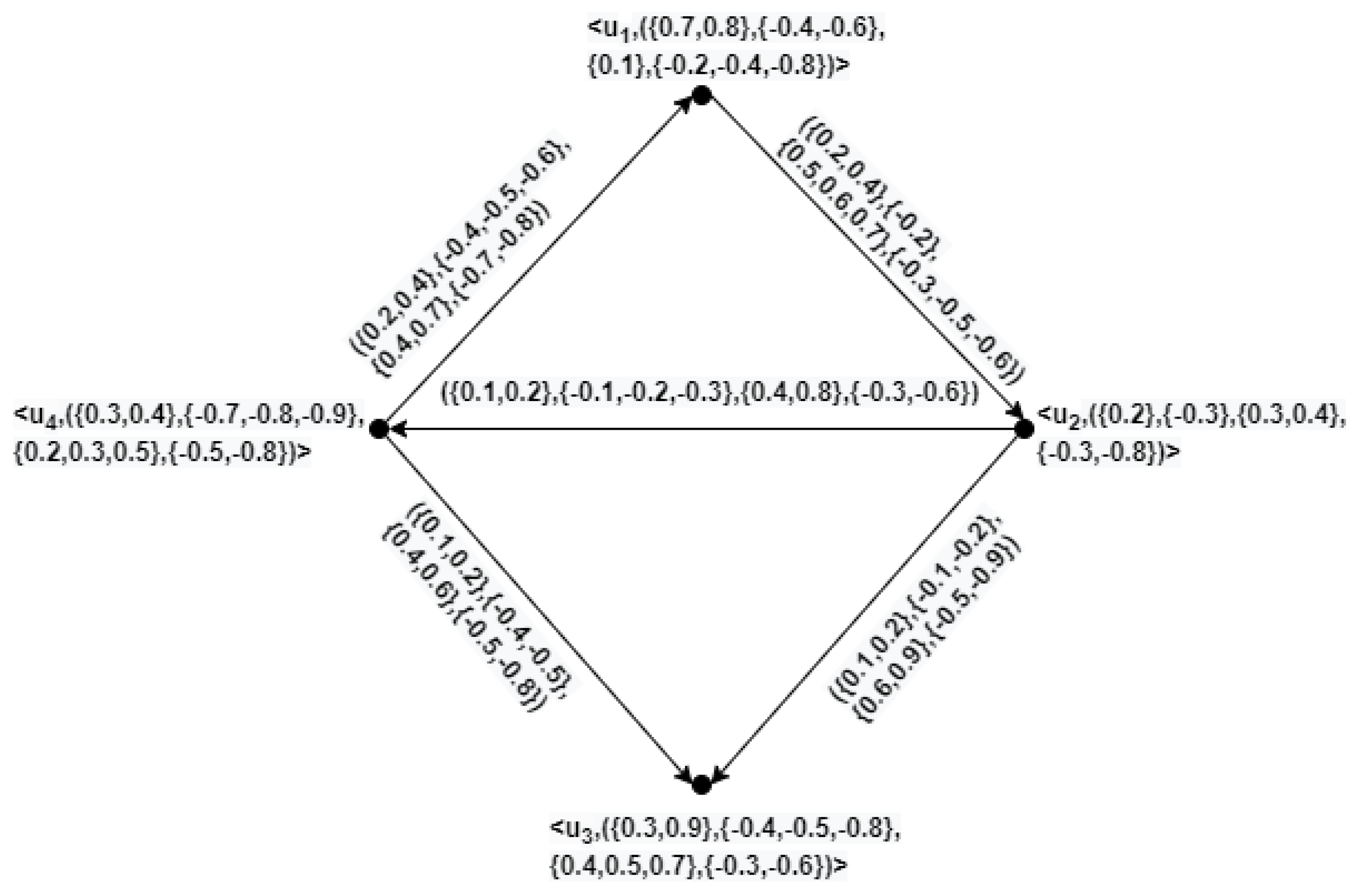
$\forall u_1,u_2\in V$. Here, R is the hesitant bipolar-valued intuitionistic fuzzy node set (HBVIFNS) of Ǧ and $\mathcal{E}$ is the hesitant bipolar-valued intuitionistic fuzzy edge set (HBVIFES) of Ǧ, respectively. Furthermore, $\mathcal{E}$ is symmetric HBVIFR on R. The elements ${\vartheta }_t^R\left(u_1\right)=(\{0,0\},\{0,0\})$ and ${\vartheta }_f^R\left(u_1\right)=(\{0,0\},\{0,0\})$ are omitted. Figure 2 shows the flowchart representation of constructing HBVIFG.

Example 7. 

Let $V=\{u_1,u_2,u_3,u_4,u_5,u_6\}$ and $E=\{(u_1,u_2),(u_2,u_3),(u_3,u_4),(u_4,u_5),(u_5,u_6),(u_3,u_6),(u_6,u_1),(u_1,u_5)\}$. The HBVIFSs $R,\mathcal{E}$ are defined as $R=\{\langle u_1,(\{0.3,0.6\},\{-0.4,-0.6\},\left\{0.2\right\},\{-0.3,-0.5,-0.6\})\rangle ,\langle u_2,(\{0.1,0.2\},\{-0.1,-0.5\},\{0.5,0.8\},\{-0.4,-0.5\})\rangle \},\langle u_3,(\{0.3,0.9\},\{-0.4,-0.5,-0.8\},\{0.4,0.5,0.7\},\{-0.3,-0.6\})\rangle ,\langle u_4,(\{0.1,0.3,0.4\},\{-0.5,-0.6\},\{0.3,0.4,0.6\},\{-0.5,-0.7\})\rangle ,\langle u_5,(\{0.2,0.4,0.6\},\{-0.5,-0.7\},\{0.2,0.5\},\{-0.1,-0.2,-0.3\})\rangle ,\langle u_6,(\{0.3,0.4\},\{-0.7,-0.8,-0.9\},\{0.2,0.3,0.5\},\{-0.5,-0.8\})\rangle \}$.

Here, ${\delta }_t\left({\vartheta }_t^R\left(u_1\right)\right)=0.475$, ${\delta }_f\left({\vartheta }_f^R\left(u_1\right)\right)=0.3334$, ${\delta }_t\left({\vartheta }_t^R\left(u_2\right)\right)=0.225$, ${\delta }_f\left({\vartheta }_f^R\left(u_2\right)\right)=0.55$, ${\delta }_t\left({\vartheta }_t^R\left(u_3\right)\right)=0.5834$, ${\delta }_f\left({\vartheta }_f^R\left(u_3\right)\right)=0.4917$, ${\delta }_t\left({\vartheta }_t^R\left(u_4\right)\right)=0.4084$, ${\delta }_f\left({\vartheta }_f^R\left(u_4\right)\right)=0.5167$, ${\delta }_t\left({\vartheta }_t^R\left(u_5\right)\right)=0.5$, ${\delta }_f\left({\vartheta }_f^R\left(u_5\right)\right)=0.275$, ${\delta }_t\left({\vartheta }_t^R\left(u_6\right)\right)=0.5750$, ${\delta }_f\left({\vartheta }_f^R\left(u_6\right)\right)=0.4917$. $\mathcal{E}=\{\langle (u_1,u_2),(\{0.1,0.2\},\{-0.1,-0.2,-0.3\},\{0.7,0.9\},\{-0.4,-0.5,-0.8\})\rangle ,\langle (u_2,u_3),(\left\{0.1\right\},\{-0.1,-0.3\},\{0.6,0.8\},\{-0.6,-0.8,-0.9\})\rangle ,\langle (u_3,u_4),(\{0.1,0.2\},\{-0.2,-0.4,-0.5\},\{0.4,0.6,0.7\},\{-0.5,-0.7,-0.9\})\rangle ,\langle (u_4,u_5),(\{0.1,0.2,0.3\},\{-0.2,-0.4\},\{0.4,0.6\},\{-0.5,-0.8\})\rangle ,\langle (u_5,u_6),(\{0.1,0.2\},\{-0.4,-0.5\},\{0.5,0.7\},\{-0.5,-0.7,-0.9\})\rangle ,\langle (u_6,u_1),(\{0.2,0.4\},\{-0.4,-0.5,-0.6\},\{0.4,0.7\},\{-0.7,-0.8\})\rangle ,\langle (u_3,u_6),(\{0.1,0.2\},\{-0.5,-0.6,-0.7\},\{0.4,0.8\},\{-0.3,-0.6\})\rangle ,\langle (u_1,u_5),(\{0.2,0.4\},\{-0.2,-0.4,-0.6\},\{0.2,0.5\},\{-0.5,-0.6,$$-0.7\left\}\right)\rangle \}$.

Here, ${\delta }_t\left({\vartheta }_t^{\mathcal{E}}(u_1,u_2)\right)=0.175$, ${\delta }_f\left({\vartheta }_f^{\mathcal{E}}(u_1,u_2)\right)=0.6834$, ${\delta }_t\left({\vartheta }_t^{\mathcal{E}}(u_2,u_3)\right)=0.15$, ${\delta }_f\left({\vartheta }_f^{\mathcal{E}}(u_2,u_3)\right)=0.7334$, ${\delta }_t\left({\vartheta }_t^{\mathcal{E}}(u_3,u_4)\right)=0.2583$, ${\delta }_f\left({\vartheta }_f^{\mathcal{E}}(u_3,u_4)\right)=0.6334$, ${\delta }_t\left({\vartheta }_t^{\mathcal{E}}(u_4,u_5)\right)=0.25$, ${\delta }_f\left({\vartheta }_f^{\mathcal{E}}(u_4,u_5)\right)=0.575$, ${\delta }_t\left({\vartheta }_t^{\mathcal{E}}(u_5,u_6)\right)=0.3$, ${\delta }_f\left({\vartheta }_f^{\mathcal{E}}(u_5,u_6)\right)=0.65$, ${\delta }_t\left({\vartheta }_t^{\mathcal{E}}(u_6,u_1)\right)=0.4$, ${\delta }_f\left({\vartheta }_f^{\mathcal{E}}(u_6,u_1)\right)=0.65$, ${\delta }_t\left({\vartheta }_t^{\mathcal{E}}(u_3,u_6)\right)=0.375$, ${\delta }_f\left({\vartheta }_f^{\mathcal{E}}(u_3,u_6)\right)=0.525$, ${\delta }_t\left({\vartheta }_t^{\mathcal{E}}(u_1,u_5)\right)=0.35$, ${\delta }_f\left({\vartheta }_f^{\mathcal{E}}(u_1,u_5)\right)=0.475$. From the above calculations, it is observed that Ǧ is a directed HBVIFG of $G=(V,E)$ and it is represented in Figure 3.

Remark 1. 

• HBVIFG is the generalization of both HBVFG and BVHFG as it can handle the uncertain information possessing membership and non-membership values along with their positive and negative aspects simultaneously.
• Furthermore, it is possible to include multiple attribute values with respect to both positive and negative sides in each of its membership and non-membership grades and thus facilitate a better understanding of uncertain/imprecise information.

Definition 18. 

Let Ǧ $=(R,\mathcal{E})$ and Ȟ $=(S,\mathcal{H})$ be a directed HBVIFG of $G=(V,E)$. Then, Ȟ $=(S,\mathcal{H})$ is called a partial directed HBVIFSG of Ǧ $=(R,\mathcal{E})$ if ${\delta }_t\left({\vartheta }_t^S\left(u_1\right)\right)\le {\delta }_t\left({\vartheta }_t^R\left(u_1\right)\right)$, ${\delta }_f\left({\vartheta }_f^S\left(u_1\right)\right)\ge {\delta }_f\left({\vartheta }_f^R\left(u_1\right)\right)$, ${\delta }_t\left({\vartheta }_t^{\mathcal{H}}(u_1,u_2)\right)\le {\delta }_t\left({\vartheta }_t^{\mathcal{E}}(u_1,u_2)\right)$ and ${\delta }_f\left({\vartheta }_f^{\mathcal{H}}(u_1,u_2)\right)\ge {\delta }_f\left({\vartheta }_f^{\mathcal{E}}(u_1,u_2)\right)$, $\forall u_1,u_2\in V$.

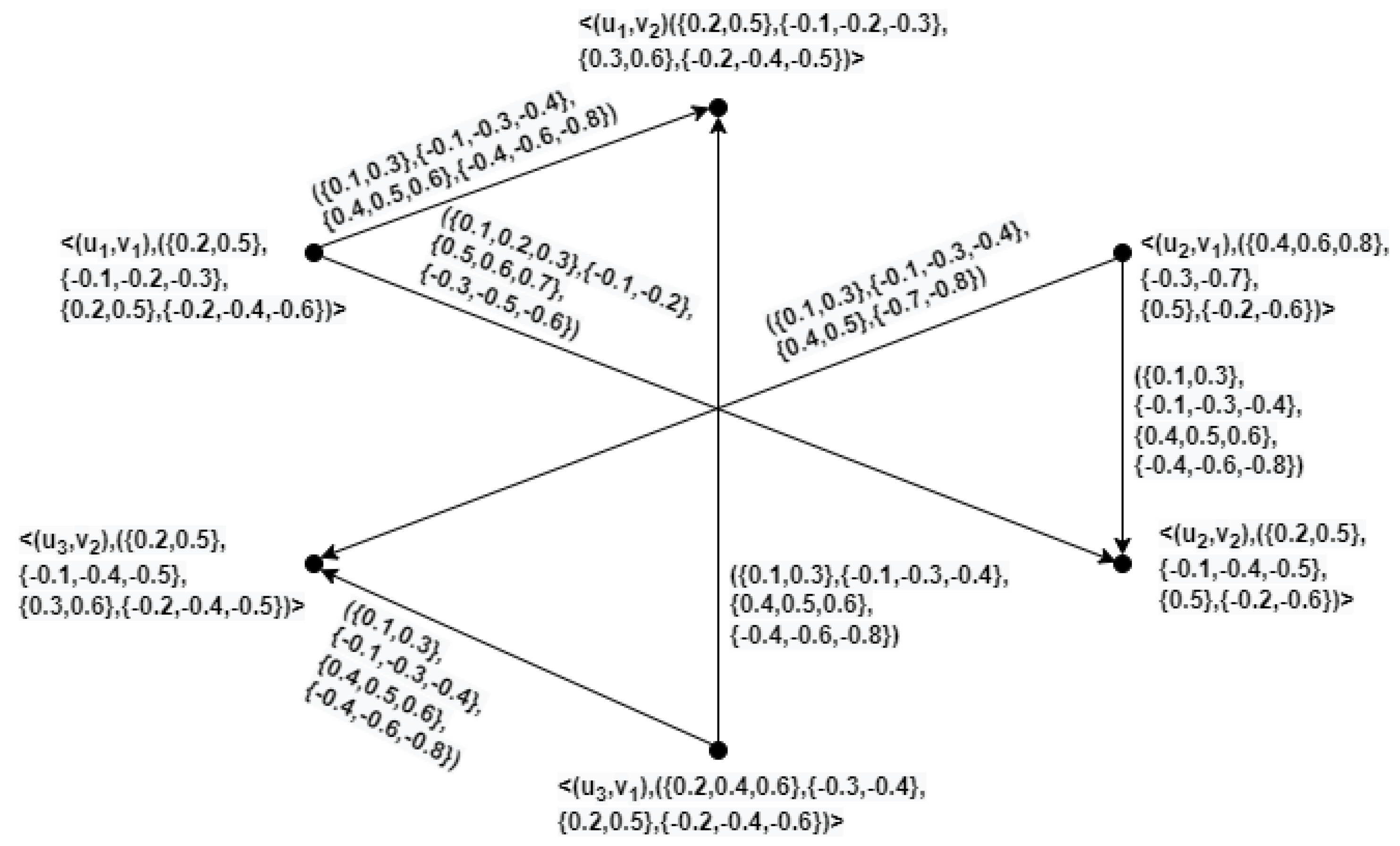
Example 8. 

Let Ȟ$=(S,\mathcal{H})$ be a directed HBVIFG of $G=(V,E)$ where $S=\{\langle u_1,(\{0.3,0.4\},$$\{-0.4,-0.6\},\{0.2,0.3\},\{-0.4,-0.6,-0.7\})\rangle ,\langle u_2,(\left\{0.2\right\},\{-0.1,-0.3\},\{0.6,0.9\},\{-0.5,$$-0.9\left\}\right)\rangle \},\langle u_3,(\{0.2,0.5\},\{-0.2,-0.4\},\{0.6,0.8\},\{-0.4,-0.8,-0.9\})\rangle ,\langle u_4,(\{0.1,0.3\},$$\{-0.2,-0.5\},\{0.4,0.5,0.7\},\{-0.6,-0.8\})\rangle ,\langle u_5,(\{0.2,0.4\},\{-0.3,-0.4\},\{0.3,0.6\},\{-0.2,$$-0.4,-0.6\left\}\right)\rangle ,\langle u_6,(\{0.1,0.2\},\{-0.4,-0.5,-0.6\},\{0.5,0.6,0.7\},\{-0.6,-0.8\})\rangle \}$.

Here, ${\delta }_t\left({\vartheta }_t^S\left(u_1\right)\right)=0.425$, ${\delta }_f\left({\vartheta }_f^S\left(u_1\right)\right)=0.4084$, ${\delta }_t\left({\vartheta }_t^S\left(u_2\right)\right)=0.2$, ${\delta }_f\left({\vartheta }_f^S\left(u_2\right)\right)=0.725$, ${\delta }_t\left({\vartheta }_t^S\left(u_3\right)\right)=0.325$, ${\delta }_f\left({\vartheta }_f^S\left(u_3\right)\right)=0.7$, ${\delta }_t\left({\vartheta }_t^S\left(u_4\right)\right)=0.275$, ${\delta }_f\left({\vartheta }_f^S\left(u_4\right)\right)=0.6167$, ${\delta }_t\left({\vartheta }_t^S\left(u_5\right)\right)=0.325$, ${\delta }_f\left({\vartheta }_f^S\left(u_5\right)\right)=0.425$, ${\delta }_t\left({\vartheta }_t^S\left(u_6\right)\right)=0.325$, ${\delta }_f\left({\vartheta }_f^S\left(u_6\right)\right)=0.65$. $\mathcal{H}=\{\langle (u_1,u_2),(\{0.1,0.2\},\{-0.1,-0.2\},\{0.7,0.8,0.9\},\{-0.6,-0.8,-0.9\})\rangle ,\langle (u_2,u_3),(\left\{0.1\right\},$$\{-0.1,-0.2\},\{0.7,0.9\},\{-0.7,-0.8,-0.9\})\rangle ,\langle (u_3,u_4),(\{0.1,0.2\},\{-0.2,-0.3\},\{0.6,0.7,0.8\},$$\{-0.5,-0.7,-0.9\})\rangle ,\langle (u_4,u_5),(\{0.1,0.2\},\{-0.1,-0.2\},\{0.5,0.8\},\{-0.6,-0.8\})\rangle ,\langle (u_5,u_6),$$(\{0.1,0.2\},\{-0.3,-0.4\},\{0.6,0.8\},\{-0.6,-0.8,-0.9\})\rangle ,\langle (u_6,u_1),(\{0.1,0.3\},\{-0.1,-0.2,$$-0.4\},\{0.6,0.8\},\{-0.7,-0.8\})\rangle ,\langle (u_3,u_6),(\{0.1,0.2\},\{-0.4,-0.5\},\{0.5,0.7\},\{-0.8,-0.9\})\rangle ,$$\langle (u_1,u_5),(\{0.1,0.3\},\{-0.1,-0.3\},\{0.5,0.8\},\{-0.6,-0.8,-0.9\})\rangle \}$.

Here, ${\delta }_t\left({\vartheta }_t^{\mathcal{H}}(u_1,u_2)\right)=0.15$, ${\delta }_f\left({\vartheta }_f^{\mathcal{H}}(u_1,u_2)\right)=0.7834$, ${\delta }_t\left({\vartheta }_t^{\mathcal{H}}(u_2,u_3)\right)=0.125$, ${\delta }_f\left({\vartheta }_f^{\mathcal{H}}(u_2,u_3)\right)=0.8$, ${\delta }_t\left({\vartheta }_t^{\mathcal{H}}(u_3,u_4)\right)=0.2$, ${\delta }_f\left({\vartheta }_f^{\mathcal{H}}(u_3,u_4)\right)=0.7$, ${\delta }_t\left({\vartheta }_t^{\mathcal{H}}(u_4,u_5)\right)=0.15$, ${\delta }_f\left({\vartheta }_f^{\mathcal{H}}(u_4,u_5)\right)=0.675$, ${\delta }_t\left({\vartheta }_t^{\mathcal{H}}(u_5,u_6)\right)=0.25$, ${\delta }_f\left({\vartheta }_f^{\mathcal{H}}(u_5,u_6)\right)=0.7334$, ${\delta }_t\left({\vartheta }_t^{\mathcal{H}}(u_6,u_1)\right)=0.1167$, ${\delta }_f\left({\vartheta }_f^{\mathcal{H}}(u_6,u_1)\right)=0.725$, ${\delta }_t\left({\vartheta }_t^{\mathcal{H}}(u_3,u_6)\right)=0.3$, ${\delta }_f\left({\vartheta }_f^{\mathcal{H}}(u_3,u_6)\right)=0.725$, ${\delta }_t\left({\vartheta }_t^{\mathcal{H}}(u_1,u_5)\right)=0.2$, ${\delta }_f\left({\vartheta }_f^{\mathcal{H}}(u_1,u_5)\right)=0.7084$.

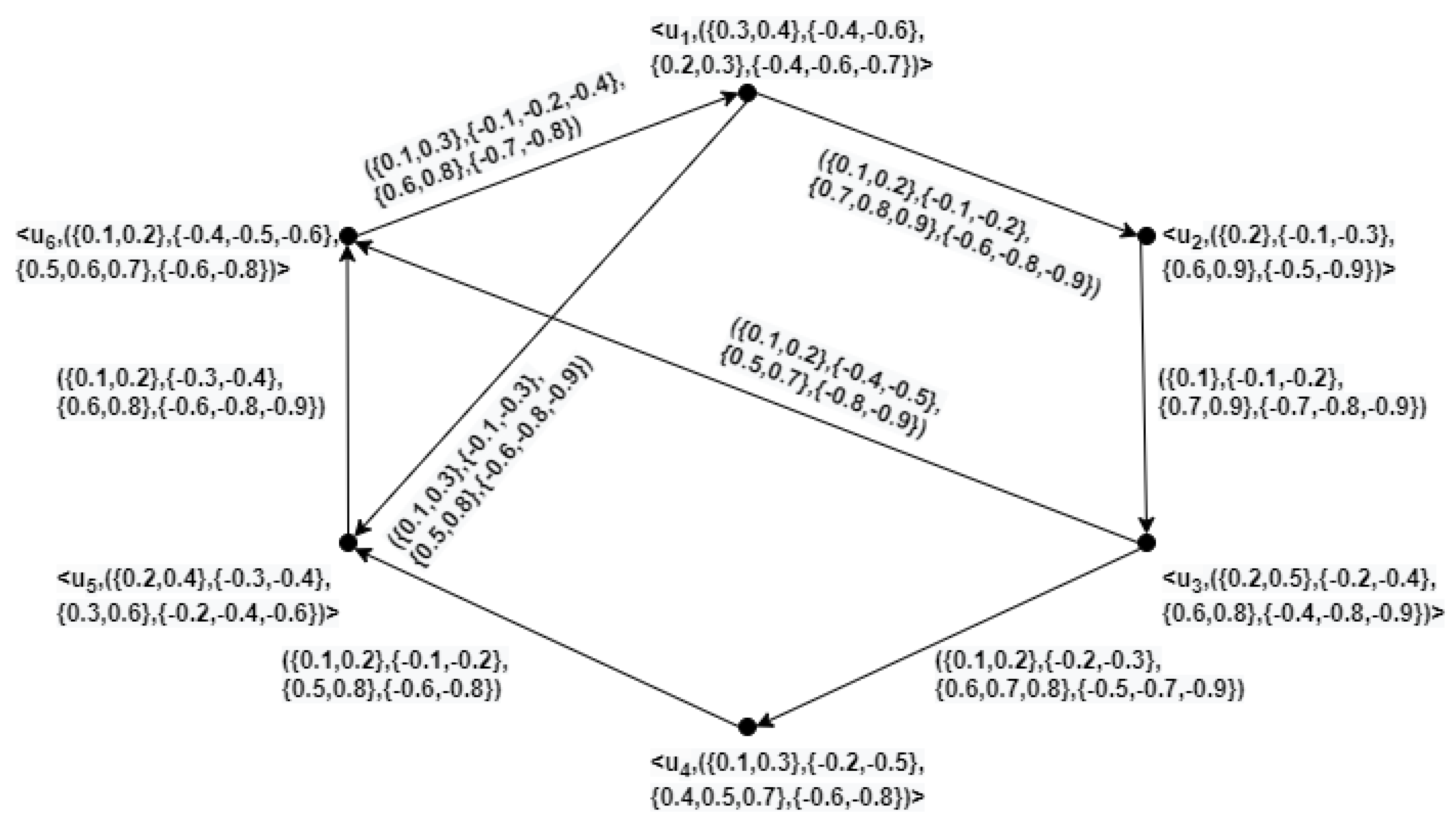
From the above calculations, it is observed that Ȟ is a partial directed HBVIFG of Ǧ $=(R,\mathcal{E})$ and is given in Figure 4.

Definition 19. 

Let Ǧ $=(R,\mathcal{E})$ and Ȟ $=(S,\mathcal{H})$ be a directed HBVIFG of $G_1=(V_1,E_1)$ and $G_2=(V_2,E_2)$. Then, Ȟ $=(S,\mathcal{H})$ is called a directed HBVIFSG of Ǧ $=(R,\mathcal{E})$ induced by $V_2$ if $V_2\subseteq V_1$, ${\delta }_t\left({\vartheta }_t^S\left(u_1\right)\right)={\delta }_t\left({\vartheta }_t^R\left(u_1\right)\right)$, ${\delta }_f\left({\vartheta }_f^S\left(u_1\right)\right)={\delta }_f\left({\vartheta }_f^R\left(u_1\right)\right)$, ${\delta }_t\left({\vartheta }_t^{\mathcal{H}}(u_1,u_2)\right)={\delta }_t\left({\vartheta }_t^{\mathcal{E}}(u_1,u_2)\right)$ and ${\delta }_f\left({\vartheta }_f^{\mathcal{H}}(u_1,u_2)\right)={\delta }_f\left({\vartheta }_f^{\mathcal{E}}(u_1,u_2)\right)$, $\forall u_1,u_2\in V_2$.

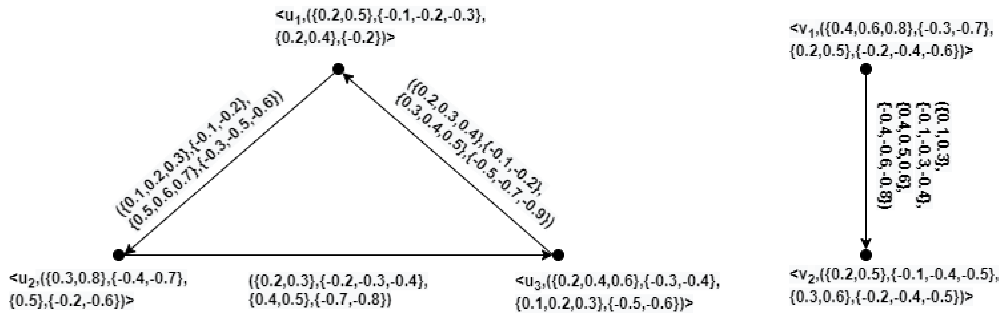
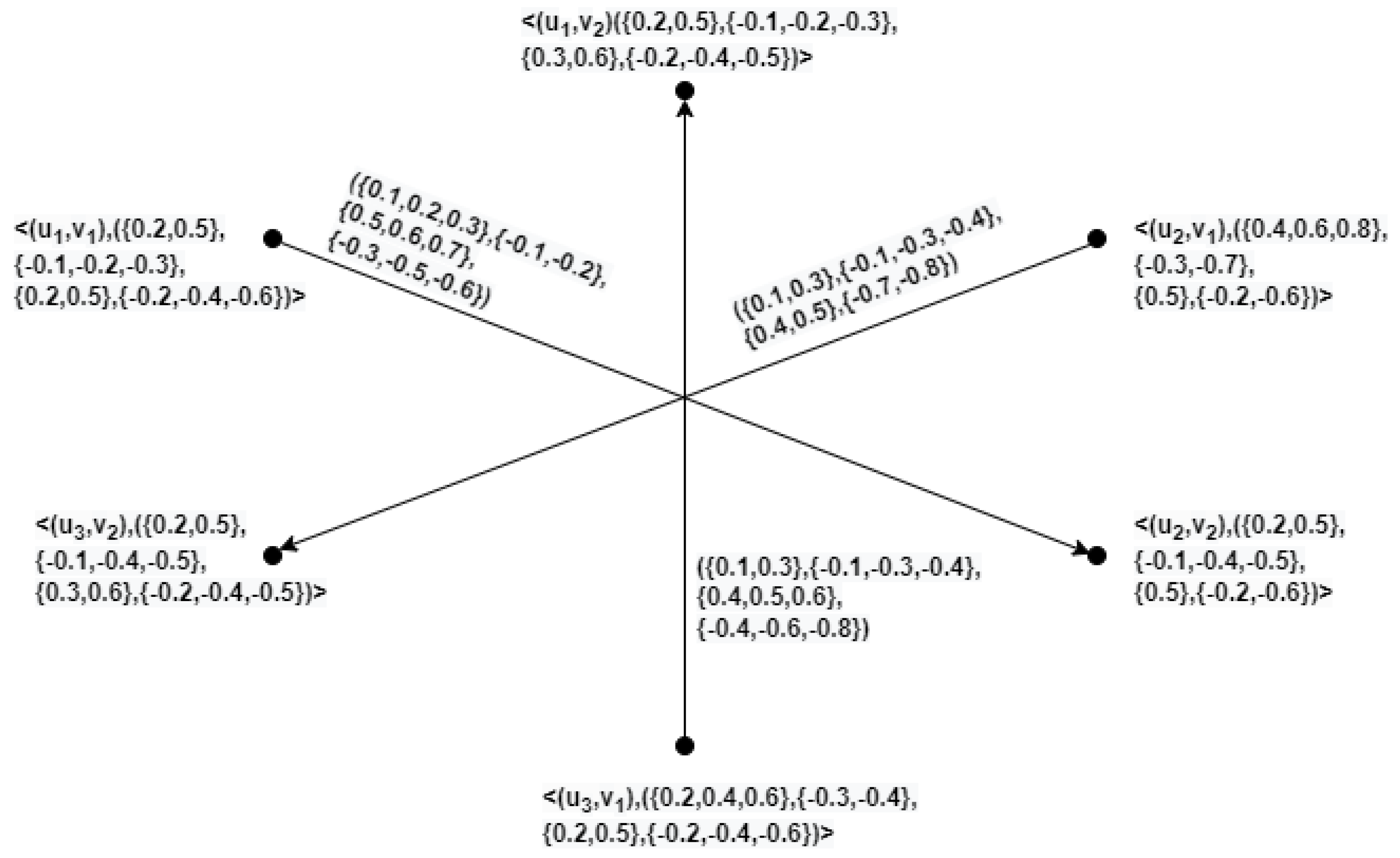
Example 9. 

Let Ǐ $=(T,\mathcal{I})$ be a directed HBVIFG of $G_1=\{V_1,E_1\}$ where $V=\{u_1,u_2,u_3,u_6\}$ and $E=\{(u_1,u_2),(u_2,u_3),(u_3,u_6),(u_6,u_1)\}$.

The HBVIFSs $R,\mathcal{E}$ are defined as $R=\{\langle u_1,(\{0.3,0.6\},\{-0.4,-0.6\},\left\{0.2\right\},\{-0.3,-0.5,$$-0.6\left\}\right)\rangle ,\langle u_2,(\{0.1,0.2\},\{-0.1,-0.5\},\{0.5,0.8\},\{-0.4,-0.5\})\rangle \},\langle u_3,(\{0.3,0.9\},\{-0.4,$$-0.5,-0.8\},\{0.4,0.5,0.7\},\{-0.3,-0.6\})\rangle ,\langle u_6,(\{0.3,0.4\},\{-0.7,-0.8,-0.9\},\{0.2,0.3,0.5\},$$\{-0.5,-0.8\})\rangle \}$.

Here, ${\delta }_t\left({\vartheta }_t^R\left(u_1\right)\right)=0.475$, ${\delta }_f\left({\vartheta }_f^R\left(u_1\right)\right)=0.3334$, ${\delta }_t\left({\vartheta }_t^R\left(u_2\right)\right)=0.225$, ${\delta }_f\left({\vartheta }_f^R\left(u_2\right)\right)=0.55$, ${\delta }_t\left({\vartheta }_t^R\left(u_3\right)\right)=0.5834$, ${\delta }_f\left({\vartheta }_f^R\left(u_3\right)\right)=0.4917$, ${\delta }_t\left({\vartheta }_t^R\left(u_6\right)\right)=0.5750$, ${\delta }_f\left({\vartheta }_f^R\left(u_6\right)\right)=0.4917$. $\mathcal{E}=\{\langle (u_1,u_2),(\{0.1,0.2\},\{-0.1,-0.2,-0.3\},\{0.7,0.9\},\{-0.4,-0.5,-0.8\})\rangle ,\langle (u_2,u_3),(\left\{0.1\right\},$$\{-0.1,-0.3\},\{0.6,0.8\},\{-0.6,-0.8,-0.9\})\rangle ,\langle (u_6,u_1),(\{0.2,0.4\},\{-0.4,-0.5,-0.6\},\{0.4,$$0.7\},\{-0.7,-0.8\})\rangle ,\langle (u_3,u_6),(\{0.1,0.2\},\{-0.5,-0.6,-0.7\},\{0.4,0.8\},\{-0.3,-0.6\})\rangle \}$.

Here, ${\delta }_t\left({\vartheta }_t^{\mathcal{E}}(u_1,u_2)\right)=0.175$, ${\delta }_f\left({\vartheta }_f^{\mathcal{E}}(u_1,u_2)\right)=0.6834$, ${\delta }_t\left({\vartheta }_t^{\mathcal{E}}(u_2,u_3)\right)=0.15$, ${\delta }_f\left({\vartheta }_f^{\mathcal{E}}(u_2,u_3)\right)=0.7334$, ${\delta }_t\left({\vartheta }_t^{\mathcal{E}}(u_6,u_1)\right)=0.4$, ${\delta }_f\left({\vartheta }_f^{\mathcal{E}}(u_6,u_1)\right)=0.65$, ${\delta }_t\left({\vartheta }_t^{\mathcal{E}}(u_3,u_6)\right)=0.375$, ${\delta }_f\left({\vartheta }_f^{\mathcal{E}}(u_3,u_6)\right)=0.525$. From the above calculations, it is observed that Ǐ is a directed HBVIFSG of Ǧ $=(R,\mathcal{E})$.

Definition 20. 

Let Ǧ $=(R,\mathcal{E})$ and Ȟ $=(S,\mathcal{H})$ be a directed HBVIFG of $G=(V,E)$. The span of Ǧ is a partial directed HBVIFSG Ȟ $=(S,\mathcal{H})$ if ${\delta }_t\left({\vartheta }_t^{\mathcal{E}}\left(u_1\right)\right)={\delta }_t\left({\vartheta }_t^{\mathcal{H}}\left(u_1\right)\right)$, ${\delta }_f\left({\vartheta }_f^{\mathcal{E}}\left(u_1\right)\right)={\delta }_f\left({\vartheta }_f^{\mathcal{H}}\left(u_1\right)\right)$, $\forall u_1\in V$. Furthermore, Ȟ $=(S,\mathcal{H})$ is called a spanning directed HBVIFSG of Ǧ $=(R,\mathcal{E})$.

Definition 21. 

A directed Ǧ $=(R,\mathcal{E})$ of $G=(V,E)$ is called a strong directed HBVIFG if ${\delta }_t\left({\vartheta }_t^{\mathcal{E}}(u_1,u_2)\right)=min\{{\delta }_t\left({\vartheta }_t^R\left(u_1\right)\right),{\delta }_t\left({\vartheta }_t^R\left(u_2\right)\right)\}$, ${\delta }_f\left({\vartheta }_f^{\mathcal{E}}(u_1,u_2)\right)=max\{{\delta }_f\left({\vartheta }_f^R\left(u_1\right)\right),{\delta }_f\left({\vartheta }_f^R\left(u_2\right)\right)\}$, $\forall (u_1,u_2)\in E$.

Definition 22. 

A directed Ǧ $=(R,\mathcal{E})$ of $G=(V,E)$ is called a complete directed HBVIFG if ${\delta }_t\left({\vartheta }_t^{\mathcal{E}}(u_1,u_2)\right)=min\{{\delta }_t\left({\vartheta }_t^R\left(u_1\right)\right),{\delta }_t\left({\vartheta }_t^R\left(u_2\right)\right)\}$, ${\delta }_f\left({\vartheta }_f^{\mathcal{E}}(u_1,u_2)\right)=max\{{\delta }_f\left({\vartheta }_f^R\left(u_1\right)\right),{\delta }_f\left({\vartheta }_f^R\left(u_2\right)\right)\}$, $\forall u_1,u_2\in V$.

4. Product of HBVIFG

This section discusses the operations of HBVIFGs. Various operations including Cartesian product, direct product, lexicographic product, and strong product are introduced. Further, it is verified that the directed HBVIFG is obtained after all these operations. In addition, the homomorphic and isomorphic mapping relations are discussed.

Definition 23. 

Let ${Ǧ}_1=(R_1,{\mathcal{E}}_1)$ and ${Ǧ}_2=(R_2,{\mathcal{E}}_2)$ be directed HBVIFGs of $G_1=(V_1,E_1)$ and $G_2=(V_2,E_2)$, respectively. Then, we have:

• The Cartesian product ${Ǧ}_1\times {Ǧ}_2=(R_1\times R_2,{\mathcal{E}}_1\times {\mathcal{E}}_2)$ of ${Ǧ}_1$ and ${Ǧ}_2$ is defined as follows:

  (a)

  $({\vartheta }_t^{R_1}\times {\vartheta }_t^{R_2})(u_1,{\nu }_1)={\vartheta }_t^{R_1}\left(u_1\right)\cap {\vartheta }_t^{R_2}\left({\nu }_1\right)$, $\forall (u_1,{\nu }_1)\in V_1\times V_2,$

  $({\vartheta }_f^{R_1}\times {\vartheta }_f^{R_2})(u_1,{\nu }_1)={\vartheta }_f^{R_1}\left(u_1\right)\cap {\vartheta }_f^{R_2}\left({\nu }_1\right)$, $\forall (u_1,{\nu }_1)\in V_1\times V_2.$

  (b)

  $({\vartheta }_t^{{\mathcal{E}}_1}\times {\vartheta }_t^{{\mathcal{E}}_2})\left((u_1,{\nu }_1)(u_1,{\nu }_2)\right)={\vartheta }_t^{R_1}\left(u_1\right)\cap {\vartheta }_t^{{\mathcal{E}}_2}({\nu }_1,{\nu }_2)$, $\forall u_1\in V_1,({\nu }_1,{\nu }_2)\in E_2,$

  $({\vartheta }_f^{{\mathcal{E}}_1}\times {\vartheta }_f^{{\mathcal{E}}_2})\left((u_1,{\nu }_1)(u_1,{\nu }_2)\right)={\vartheta }_f^{R_1}\left(u_1\right)\cap {\vartheta }_f^{{\mathcal{E}}_2}({\nu }_1,{\nu }_2)$, $\forall u_1\in V_1,({\nu }_1,{\nu }_2)\in E_2.$

  (c)

  $({\vartheta }_t^{{\mathcal{E}}_1}\times {\vartheta }_t^{{\mathcal{E}}_2})\left((u_1,{\nu }_1)(u_2,{\nu }_1)\right)={\vartheta }_t^{{\mathcal{E}}_1}(u_1,u_2)\cap {\vartheta }_t^{R_2}\left({\nu }_1\right)$, $\forall (u_1,u_2)\in E_1,{\nu }_1\in V_2,$

  $({\vartheta }_f^{{\mathcal{E}}_1}\times {\vartheta }_f^{{\mathcal{E}}_2})\left((u_1,{\nu }_1)(u_2,{\nu }_1)\right)={\vartheta }_f^{{\mathcal{E}}_1}(u_1,u_2)\cap {\vartheta }_f^{R_2}\left({\nu }_1\right)$, $\forall (u_1,u_2)\in E_1,{\nu }_1\in V_2.$

• The direct product ${Ǧ}_1\ast {Ǧ}_2=(R_1\ast R_2,{\mathcal{E}}_1\ast {\mathcal{E}}_2)$ of ${Ǧ}_1$ and ${Ǧ}_2$ is defined as follows:

  (a)

  $({\vartheta }_t^{R_1}*{\vartheta }_t^{R_2})(u_1,{\nu }_1)={\vartheta }_t^{R_1}\left(u_1\right)\cap {\vartheta }_t^{R_2}\left({\nu }_1\right)$, $\forall (u_1,{\nu }_1)\in V_1\times V_2,$

  $({\vartheta }_f^{R_1}\ast {\vartheta }_f^{R_2})(u_1,{\nu }_1)={\vartheta }_f^{R_1}\left(u_1\right)\cap {\vartheta }_f^{R_2}\left({\nu }_1\right)$, $\forall (u_1,{\nu }_1)\in V_1\times V_2.$

  (b)

  $({\vartheta }_t^{{\mathcal{E}}_1}\ast {\vartheta }_t^{{\mathcal{E}}_2})\left((u_1,{\nu }_1)(u_2,{\nu }_2)\right)={\vartheta }_t^{{\mathcal{E}}_1}(u_1,u_2)\cap {\vartheta }_t^{{\mathcal{E}}_2}({\nu }_1,{\nu }_2)$, $\forall (u_1,u_2)\in E_1,({\nu }_1,{\nu }_2)\in E_2,$

  $({\vartheta }_f^{{\mathcal{E}}_1}\ast {\vartheta }_f^{{\mathcal{E}}_2})\left((u_1,{\nu }_1)(u_2,{\nu }_2)\right)={\vartheta }_f^{{\mathcal{E}}_1}(u_1,u_2)\cap {\vartheta }_f^{{\mathcal{E}}_2}({\nu }_1,{\nu }_2)$, $\forall (u_1,u_2)\in E_1,({\nu }_1,{\nu }_2)\in E_2.$

• The lexicographic product ${Ǧ}_1\odot {Ǧ}_2=(R_1\odot R_2,{\mathcal{E}}_1\odot {\mathcal{E}}_2)$ of ${Ǧ}_1$ and ${Ǧ}_2$ is defined as follows:

  (a)

  $({\vartheta }_t^{R_1}\odot {\vartheta }_t^{R_2})(u_1,{\nu }_1)={\vartheta }_t^{R_1}\left(u_1\right)\cap {\vartheta }_t^{R_2}\left({\nu }_1\right)$, $\forall (u_1,{\nu }_1)\in V_1\times V_2,$

  $({\vartheta }_f^{R_1}\odot {\vartheta }_f^{R_2})(u_1,{\nu }_1)={\vartheta }_f^{R_1}\left(u_1\right)\cap {\vartheta }_f^{R_2}\left({\nu }_1\right)$, $\forall (u_1,{\nu }_1)\in V_1\times V_2.$

  (b)

  $({\vartheta }_t^{{\mathcal{E}}_1}\odot {\vartheta }_t^{{\mathcal{E}}_2})\left((u_1,{\nu }_1)(u_1,{\nu }_2)\right)={\vartheta }_t^{R_1}\left(u_1\right)\cap {\vartheta }_t^{{\mathcal{E}}_2}({\nu }_1,{\nu }_2)$, $\forall u_1\in V_1,({\nu }_1,{\nu }_2)\in E_2,$

  $({\vartheta }_f^{{\mathcal{E}}_1}\odot {\vartheta }_f^{{\mathcal{E}}_2})\left((u_1,{\nu }_1)(u_1,{\nu }_2)\right)={\vartheta }_f^{R_1}\left(u_1\right)\cap {\vartheta }_f^{{\mathcal{E}}_2}({\nu }_1,{\nu }_2)$, $\forall u_1\in V_1,({\nu }_1,{\nu }_2)\in E_2.$

  (c)

  $({\vartheta }_t^{{\mathcal{E}}_1}\odot {\vartheta }_t^{{\mathcal{E}}_2})\left((u_1,{\nu }_1)(u_2,{\nu }_2)\right)={\vartheta }_t^{{\mathcal{E}}_1}(u_1,u_2)\cap {\vartheta }_t^{{\mathcal{E}}_2}({\nu }_1,{\nu }_2)$, $\forall (u_1,u_2)\in E_1,({\nu }_1,{\nu }_2)\in E_2,$

  $({\vartheta }_f^{{\mathcal{E}}_1}\odot {\vartheta }_f^{{\mathcal{E}}_2})\left((u_1,{\nu }_1)(u_2,{\nu }_2)\right)={\vartheta }_f^{{\mathcal{E}}_1}(u_1,u_2)\cap {\vartheta }_f^{{\mathcal{E}}_2}({\nu }_1,{\nu }_2)$, $\forall (u_1,u_2)\in E_1,({\nu }_1,{\nu }_2)\in E_2.$

• The strong product ${Ǧ}_1\otimes {Ǧ}_2=(R_1\otimes R_2,{\mathcal{E}}_1\otimes {\mathcal{E}}_2)$ of ${Ǧ}_1$ and ${Ǧ}_2$ is defined as follows:

  (a)

  $({\vartheta }_t^{R_1}\otimes {\vartheta }_t^{R_2})(u_1,{\nu }_1)={\vartheta }_t^{R_1}\left(u_1\right)\cap {\vartheta }_t^{R_2}\left({\nu }_1\right)$, $\forall (u_1,{\nu }_1)\in V_1\times V_2,$

  $({\vartheta }_f^{R_1}\otimes {\vartheta }_f^{R_2})(u_1,{\nu }_1)={\vartheta }_f^{R_1}\left(u_1\right)\cap {\vartheta }_f^{R_2}\left({\nu }_1\right)$, $\forall (u_1,{\nu }_1)\in V_1\times V_2.$

  (b)

  $({\vartheta }_t^{{\mathcal{E}}_1}\otimes {\vartheta }_t^{{\mathcal{E}}_2})\left((u_1,{\nu }_1)(u_1,{\nu }_2)\right)={\vartheta }_t^{R_1}\left(u_1\right)\cap {\vartheta }_t^{{\mathcal{E}}_2}({\nu }_1,{\nu }_2)$, $\forall u_1\in V_1,({\nu }_1,{\nu }_2)\in E_2,$

  $({\vartheta }_f^{{\mathcal{E}}_1}\otimes {\vartheta }_f^{{\mathcal{E}}_2})\left((u_1,{\nu }_1)(u_1,{\nu }_2)\right)={\vartheta }_f^{R_1}\left(u_1\right)\cap {\vartheta }_f^{{\mathcal{E}}_2}({\nu }_1,{\nu }_2)$, $\forall u_1\in V_1,({\nu }_1,{\nu }_2)\in E_2.$

  (c)

  $({\vartheta }_t^{{\mathcal{E}}_1}\otimes {\vartheta }_t^{{\mathcal{E}}_2})\left((u_1,{\nu }_1)(u_2,{\nu }_1)\right)={\vartheta }_t^{{\mathcal{E}}_1}(u_1,u_2)\cap {\vartheta }_t^{R_2}\left({\nu }_1\right)$, $\forall (u_1,u_2)\in E_1,{\nu }_1\in V_2,$

  $({\vartheta }_f^{{\mathcal{E}}_1}\otimes {\vartheta }_f^{{\mathcal{E}}_2})\left((u_1,{\nu }_1)(u_2,{\nu }_1)\right)={\vartheta }_f^{{\mathcal{E}}_1}(u_1,u_2)\cap {\vartheta }_f^{R_2}\left({\nu }_1\right)$, $\forall (u_1,u_2)\in E_1,{\nu }_1\in V_2.$

  (d)

  $({\vartheta }_t^{{\mathcal{E}}_1}\otimes {\vartheta }_t^{{\mathcal{E}}_2})\left((u_1,{\nu }_1)(u_2,{\nu }_2)\right)={\vartheta }_t^{{\mathcal{E}}_1}(u_1,u_2)\cap {\vartheta }_t^{{\mathcal{E}}_2}({\nu }_1,{\nu }_2)$, $\forall (u_1,u_2)\in E_1,({\nu }_1,{\nu }_2)\in E_2,$

  $({\vartheta }_f^{{\mathcal{E}}_1}\otimes {\vartheta }_f^{{\mathcal{E}}_2})\left((u_1,{\nu }_1)(u_2,{\nu }_2)\right)={\vartheta }_f^{{\mathcal{E}}_1}(u_1,u_2)\cap {\vartheta }_f^{{\mathcal{E}}_2}({\nu }_1,{\nu }_2)$, $\forall (u_1,u_2)\in E_1,({\nu }_1,{\nu }_2)\in E_2.$

Example 10. 

Let ${Ǧ}_1=(R_1,{\mathcal{E}}_1)$ and ${Ǧ}_2=(R_2,{\mathcal{E}}_2)$ be two directed HBVIFGs as given in Figure 5. Then, ${Ǧ}_1\times {Ǧ}_2$, ${Ǧ}_1\ast {Ǧ}_2$, ${Ǧ}_1\odot {Ǧ}_2$, and ${Ǧ}_1\otimes {Ǧ}_2$ of ${Ǧ}_1$ and ${Ǧ}_2$ are represented in Figure 6, Figure 7, Figure 8, and Figure 9, respectively.

Theorem 1. 

Let ${Ǧ}_1=(R_1,{\mathcal{E}}_1)$ and ${Ǧ}_2=(R_2,{\mathcal{E}}_2)$ be directed HBVIFGs of $G_1=(V_1,E_1)$ and $G_2=(V_2,E_2)$, respectively. Then,

• ${Ǧ}_1\times {Ǧ}_2=(R_1\times R_2,{\mathcal{E}}_1\times {\mathcal{E}}_2)$ is a directed HBVIFG of $G_1\times G_2$.
• ${Ǧ}_1\ast {Ǧ}_2=(R_1\ast R_2,{\mathcal{E}}_1\ast {\mathcal{E}}_2)$ is a directed HBVIFG of $G_1\times G_2$.
• ${Ǧ}_1\odot {Ǧ}_2=(R_1\odot R_2,{\mathcal{E}}_1\odot {\mathcal{E}}_2)$ is a directed HBVIFG of $G_1\times G_2$.
• ${Ǧ}_1\otimes {Ǧ}_2=(R_1\otimes R_2,{\mathcal{E}}_1\otimes {\mathcal{E}}_2)$ is a directed HBVIFG of $G_1\times G_2$.

Proof. 

(1) Case 1 For all $(u_1,{\nu }_1)\in V_1\times V_2$, we have

$$\begin{array}{cc}\hfill {\delta }_t\left(({\vartheta }_t^{R_1}\times {\vartheta }_t^{R_2})(u_1,{\nu }_1)\right)& ={\delta }_t({\vartheta }_t^{R_1}\left(u_1\right)\cap {\vartheta }_t^{R_2}\left({\nu }_1\right)),\hfill \\ \hfill & =min\{{\delta }_t\left({\vartheta }_t^{R_1}\left(u_1\right)\right),{\delta }_t\left({\vartheta }_t^{R_2}\left({\nu }_1\right)\right)\}\hfill \end{array}$$

$$\begin{array}{cc}\hfill {\delta }_f\left(({\vartheta }_f^{R_1}\times {\vartheta }_f^{R_2})(u_1,{\nu }_1)\right)& ={\delta }_f({\vartheta }_f^{R_1}\left(u_1\right)\cap {\vartheta }_f^{R_2}\left({\nu }_1\right)),\hfill \\ \hfill & =max\{{\delta }_f\left({\vartheta }_f^{R_1}\left(u_1\right)\right),{\delta }_f\left({\vartheta }_f^{R_2}\left({\nu }_1\right)\right)\}\hfill \end{array}$$

Case 2 Let $u_1\in V_1,({\nu }_1,{\nu }_2)\in E_2$, then,

$$\begin{array}{cc}\hfill {\delta }_t\left(({\vartheta }_t^{{\mathcal{E}}_1}\times {\vartheta }_t^{{\mathcal{E}}_2})\right((u_1,{\nu }_1)& (u_1,{\nu }_2)\left)\right)={\delta }_t({\vartheta }_t^{R_1}\left(u_1\right)\cap {\vartheta }_t^{{\mathcal{E}}_2}({\nu }_1,{\nu }_2)),\hfill \\ \hfill & =min\{{\delta }_t\left({\vartheta }_t^{R_1}\left(u_1\right)\right),{\delta }_t\left({\vartheta }_t^{{\mathcal{E}}_2}({\nu }_1,{\nu }_2)\right)\},\hfill \\ \hfill & \le min\{{\delta }_t\left({\vartheta }_t^{R_1}\left(u_1\right)\right),min\{{\delta }_t\left({\vartheta }_t^{R_2}\left({\nu }_1\right)\right),{\delta }_t\left({\vartheta }_t^{R_2}\left({\nu }_2\right)\right)\}\},\hfill \\ \hfill & =min\{min\{{\delta }_t\left({\vartheta }_t^{R_1}\left(u_1\right)\right),{\delta }_t\left({\vartheta }_t^{R_2}\left({\nu }_1\right)\right)\},min\{{\delta }_t\left({\vartheta }_t^{R_1}\left(u_1\right)\right),{\delta }_t\left({\vartheta }_t^{R_2}\left({\nu }_2\right)\right)\}\},\hfill \\ \hfill & =min\{{\delta }_t({\vartheta }_t^{R_1}\left(u_1\right)\cap {\vartheta }_t^{R_2}\left({\nu }_1\right)),{\delta }_t({\vartheta }_t^{R_1}\left(u_1\right)\cap {\vartheta }_t^{R_2}\left({\nu }_2\right))\},\hfill \\ \hfill & =min\{{\delta }_t\left(({\vartheta }_t^{R_1}\times {\vartheta }_t^{R_2})(u_1,{\nu }_1)\right),{\delta }_t\left(({\vartheta }_t^{R_1}\times {\vartheta }_t^{R_2})(u_1,{\nu }_2)\right)\}.\hfill \end{array}$$

$$\begin{array}{cc}\hfill {\delta }_f\left(({\vartheta }_f^{{\mathcal{E}}_1}\times {\vartheta }_f^{{\mathcal{E}}_2})\right((u_1,{\nu }_1)& (u_1,{\nu }_2)\left)\right)={\delta }_f({\vartheta }_f^{R_1}\left(u_1\right)\cap {\vartheta }_f^{{\mathcal{E}}_2}({\nu }_1,{\nu }_2)),\hfill \\ \hfill & =max\{{\delta }_f\left({\vartheta }_f^{R_1}\left(u_1\right)\right),{\delta }_f\left({\vartheta }_t^{{\mathcal{E}}_2}({\nu }_1,{\nu }_2)\right)\},\hfill \\ \hfill & \ge max\{{\delta }_f\left({\vartheta }_f^{R_1}\left(u_1\right)\right),max\{{\delta }_f\left({\vartheta }_f^{R_2}\left({\nu }_1\right)\right),{\delta }_f\left({\vartheta }_f^{R_2}\left({\nu }_2\right)\right)\}\},\hfill \\ \hfill & =max\{max\{{\delta }_f\left({\vartheta }_f^{R_1}\left(u_1\right)\right),{\delta }_f\left({\vartheta }_f^{R_2}\left({\nu }_1\right)\right)\},max\{{\delta }_f\left({\vartheta }_f^{R_1}\left(u_1\right)\right),{\delta }_f\left({\vartheta }_f^{R_2}\left({\nu }_2\right)\right)\}\},\hfill \\ \hfill & =max\{{\delta }_f({\vartheta }_f^{R_1}\left(u_1\right)\cap {\vartheta }_f^{R_2}\left({\nu }_1\right)),{\delta }_f({\vartheta }_f^{R_1}\left(u_1\right)\cap {\vartheta }_f^{R_2}\left({\nu }_2\right))\},\hfill \\ \hfill & =max\{{\delta }_f\left(({\vartheta }_f^{R_1}\times {\vartheta }_f^{R_2})(u_1,{\nu }_1)\right),{\delta }_f\left(({\vartheta }_f^{R_1}\times {\vartheta }_f^{R_2})(u_1,{\nu }_2)\right)\}.\hfill \end{array}$$

Case 3 Let $(u_1,u_2)\in E_1,{\nu }_1\in V_2,$

$$\begin{array}{cc}\hfill {\delta }_t\left(({\vartheta }_t^{{\mathcal{E}}_1}\times {\vartheta }_t^{{\mathcal{E}}_2})\right((u_1,{\nu }_1)& (u_2,{\nu }_1)\left)\right)={\delta }_t({\vartheta }_t^{{\mathcal{E}}_1}(u_1,u_2)\cap {\vartheta }_t^{R_2}\left({\nu }_1\right)),\hfill \\ \hfill & =min\{{\delta }_t\left({\vartheta }_t^{{\mathcal{E}}_1}(u_1,u_2)\right),{\delta }_t\left({\vartheta }_t^{R_2}\left({\nu }_1\right)\right)\},\hfill \\ \hfill & \le min\{min\{{\delta }_t\left({\vartheta }_t^{R_1}\left(u_1\right)\right),{\delta }_t\left({\vartheta }_t^{R_1}\left(u_2\right)\right)\},{\delta }_t\left({\vartheta }_t^{R_2}\left({\nu }_1\right)\right)\},\hfill \\ \hfill & =min\{min\{{\delta }_t\left({\vartheta }_t^{R_1}\left(u_1\right)\right),{\delta }_t\left({\vartheta }_t^{R_2}\left({\nu }_1\right)\right)\},min\{{\delta }_t\left({\vartheta }_t^{R_1}\left(u_2\right)\right),{\delta }_t\left({\vartheta }_t^{R_2}\left({\nu }_1\right)\right)\}\},\hfill \\ \hfill & =min\{{\delta }_t({\vartheta }_t^{R_1}\left(u_1\right)\cap {\vartheta }_t^{R_2}\left({\nu }_1\right)),{\delta }_t({\vartheta }_t^{R_1}\left(u_2\right)\cap {\vartheta }_t^{R_2}\left({\nu }_1\right))\},\hfill \\ \hfill & =min\{{\delta }_t\left(({\vartheta }_t^{R_1}\times {\vartheta }_t^{R_2})(u_1,{\nu }_1)\right),{\delta }_t\left(({\vartheta }_t^{R_1}\times {\vartheta }_t^{R_2})(u_2,{\nu }_1)\right)\}.\hfill \end{array}$$

$$\begin{array}{cc}\hfill {\delta }_f\left(({\vartheta }_f^{{\mathcal{E}}_1}\times {\vartheta }_f^{{\mathcal{E}}_2})\right((u_1,{\nu }_1)& (u_2,{\nu }_1)\left)\right)={\delta }_f({\vartheta }_f^{{\mathcal{E}}_1}(u_1,u_2)\cap {\vartheta }_f^{R_2}\left({\nu }_1\right)),\hfill \\ \hfill & =max\{{\delta }_f\left({\vartheta }_f^{{\mathcal{E}}_1}(u_1,u_2)\right),{\delta }_f\left({\vartheta }_f^{R_2}\left({\nu }_1\right)\right)\},\hfill \\ \hfill & \ge max\{max\{{\delta }_f\left({\vartheta }_f^{R_1}\left(u_1\right)\right),{\delta }_f\left({\vartheta }_f^{R_1}\left(u_2\right)\right)\},{\delta }_f\left({\vartheta }_f^{R_2}\left({\nu }_1\right)\right)\},\hfill \\ \hfill & =max\{max\{{\delta }_f\left({\vartheta }_f^{R_1}\left(u_1\right)\right),{\delta }_f\left({\vartheta }_f^{R_2}\left({\nu }_1\right)\right)\},max\{{\delta }_f\left({\vartheta }_f^{R_1}\left(u_2\right)\right),{\delta }_f\left({\vartheta }_f^{R_2}\left({\nu }_1\right)\right)\}\},\hfill \\ \hfill & =max\{{\delta }_f({\vartheta }_f^{R_1}\left(u_1\right)\cap {\vartheta }_f^{R_2}\left({\nu }_1\right)),{\delta }_f({\vartheta }_f^{R_1}\left(u_2\right)\cap {\vartheta }_f^{R_2}\left({\nu }_1\right))\},\hfill \\ \hfill & =max\{{\delta }_f\left(({\vartheta }_f^{R_1}\times {\vartheta }_f^{R_2})(u_1,{\nu }_1)\right),{\delta }_f\left(({\vartheta }_f^{R_1}\times {\vartheta }_f^{R_2})(u_2,{\nu }_1)\right)\}.\hfill \end{array}$$

From Case 1, 2, and 3, ${\mathrm{Ǧ}}_1\times {\mathrm{Ǧ}}_2=(R_1\times R_2,{\mathcal{E}}_1\times {\mathcal{E}}_2)$ is a directed HBVIFG of $G_1\times G_2$. The remaining operations can be proved in a similar way.    □

Note The working procedure of Theorem 1 is given here. For instance, from Figure 5 and Figure 6, consider, $\langle u_1,(\{0.2,0.5\},\{-0.1,-0.2,-0.3\},\{0.2,0.4\},\{-0.2\})\rangle \in R_1$, ${\nu }_1,$$(\{0.4,0.8,0.6\},\{-0.3,-0.7\},\{0.2,0.5\},\{-0.2,-0.4,-0.6\})\rangle \in R_2$, ${\nu }_2,(\{0.2,0.5\},\{-0.1,-0.4,$$-0.5\},\{0.6,0.3\},\{-0.2,-0.4,-0.5\})\rangle \in R_2$ and $\langle (u_1,{\nu }_1),(\{0.2,0.5\},\{-0.1,-0.2,-0.3\},\{0.2,$$0.5\},\{-0.2,-0.4,-0.6\})\rangle \in R_1\times R_2$, $\langle (u_1,{\nu }_2),(\{0.2,0.5\},\{-0.1,-0.2,-0.3\},\{0.3,0.6\},\{-0.2,$$-0.4,-0.5\left\}\right)\rangle \in R_1\times R_2$ and $\langle ((u_1,{\nu }_1),(u_1,{\nu }_2)),(\{0.1,0.3\},\{-0.1,-0.3,-0.4\},\{0.4,0.5,0.6\},$$\{-0.8,-0.4,-0.6\})\rangle \in {\mathcal{E}}_1\times {\mathcal{E}}_2$. Their HBVIFSVs and HBVIFNSVs are ${\delta }_t\left({\vartheta }_t^{R_1}\left(u_1\right)\right)=0.275$, ${\delta }_f\left({\vartheta }_f^{R_1}\left(u_1\right)\right)=0.25$, ${\delta }_t\left({\vartheta }_t^{R_2}\left({\nu }_1\right)\right)=0.55$, ${\delta }_f\left({\vartheta }_f^{R_2}\left({\nu }_1\right)\right)=0.3333$, ${\delta }_t\left({\vartheta }_t^{R_2}\left({\nu }_2\right)\right)=0.3417$, ${\delta }_f\left({\vartheta }_f^{R_2}\left({\nu }_2\right)\right)=0.4084$, ${\delta }_t\left(({\vartheta }_t^{R_1}\times {\vartheta }_t^{R_2})(u_1,{\nu }_1)\right)=0.275$, ${\delta }_f\left(({\vartheta }_f^{R_1}\times {\vartheta }_f^{R_2})(u_1,{\nu }_1)\right)=0.375$, ${\delta }_t\left(({\vartheta }_t^{R_1}\times {\vartheta }_t^{R_2})(u_1,{\nu }_2)\right)=0.275$, ${\delta }_f\left(({\vartheta }_f^{R_1}\times {\vartheta }_f^{R_2})(u_1,{\nu }_2)\right)=0.4084$, ${\delta }_t\left(({\vartheta }_t^{{\mathcal{E}}_1}\times {\vartheta }_t^{{\mathcal{E}}_2})\right((u_1,{\nu }_1)$$(u_1,{\nu }_2)\left)\right)=0.2334$ and ${\delta }_f\left(({\vartheta }_f^{{\mathcal{E}}_1}\times {\vartheta }_f^{{\mathcal{E}}_2})\left((u_1,{\nu }_1)(u_1,{\nu }_2)\right)\right)=0.55$. To check whether these HBVIFEs satisfy the minimality and maximality conditions provided in Definition 17, we employ Theorem 1. We have ${\delta }_t\left(({\vartheta }_t^{{\mathcal{E}}_1}\times {\vartheta }_t^{{\mathcal{E}}_2})\left((u_1,{\nu }_1)(u_1,{\nu }_2)\right)\right)=0.2334$. From Theorem 1, Case 2, we have

$$\begin{array}{cc}\hfill {\delta }_t\left(({\vartheta }_t^{{\mathcal{E}}_1}\times {\vartheta }_t^{{\mathcal{E}}_2})\left((u_1,{\nu }_1)(u_1,{\nu }_2)\right)\right)& =0.2334\hfill \\ \hfill & \le min\{{\delta }_t\left(({\vartheta }_t^{R_1}\times {\vartheta }_t^{R_2})(u_1,{\nu }_1)\right),{\delta }_t\left(({\vartheta }_t^{R_1}\times {\vartheta }_t^{R_2})(u_1,{\nu }_2)\right)\}\hfill \\ \hfill & =min\{0.275,0.275\}=0.275.\hfill \end{array}$$

Similarly,

$$\begin{array}{cc}\hfill {\delta }_f\left(({\vartheta }_f^{{\mathcal{E}}_1}\times {\vartheta }_f^{{\mathcal{E}}_2})\left((u_1,{\nu }_1)(u_1,{\nu }_2)\right)\right)& =0.55\hfill \\ \hfill & \ge max\{{\delta }_f\left(({\vartheta }_f^{R_1}\times {\vartheta }_f^{R_2})(u_1,{\nu }_1)\right),{\delta }_f\left(({\vartheta }_f^{R_1}\times {\vartheta }_f^{R_2})(u_1,{\nu }_2)\right)\}\hfill \\ \hfill & =max\{0.375,0.4084\}=0.4084.\hfill \end{array}$$

Thus, the minimality and maximality conditions provided in Definition 17 is satisfied using Theorem 1. The other minimality and maximality conditions can be obtained in the same manner. Thus, ${\mathrm{Ǧ}}_1\times {\mathrm{Ǧ}}_2$ is the resulting directed HBVIFG obtained using Theorem 1.

Definition 24. 

Let ${Ǧ}_1=(R_1,{\mathcal{E}}_1)$ and ${Ǧ}_2=(R_2,{\mathcal{E}}_2)$ be directed HBVIFGs of $G_1=(V_1,E_1)$ and $G_2=(V_2,E_2)$, respectively. Then, the mapping relationships of directed HBVIFGs are defined as follows:

• The homomorphism between ${Ǧ}_1$ and ${Ǧ}_2$ is a bijective mapping $g:V_1\to V_2$ which satisfies

  (a)

  ${\delta }_t\left({\vartheta }_t^{R_1}\left(u_1\right)\right)\le {\delta }_t\left({\vartheta }_t^{R_2}\left(g\left(u_1\right)\right)\right)$

  ${\delta }_f\left({\vartheta }_f^{R_1}\left(u_1\right)\right)\ge {\delta }_f\left({\vartheta }_f^{R_2}\left(g\left(u_1\right)\right)\right)$, $\forall u_1\in V_1$.

  (b)

  ${\delta }_t\left({\vartheta }_t^{{\mathcal{E}}_1}(u_1,u_2)\right)\le {\delta }_t\left({\vartheta }_t^{{\mathcal{E}}_2}(g\left(u_1\right),g\left(u_2\right))\right)$

  ${\delta }_f\left({\vartheta }_t^{{\mathcal{E}}_1}(u_1,u_2)\right)\ge {\delta }_f\left({\vartheta }_f^{{\mathcal{E}}_2}(g\left(u_1\right),g\left(u_2\right))\right)$, $\forall u_1,u_2\in V_1$.

• The isomorphism between ${Ǧ}_1$ and ${Ǧ}_2$ is a bijective mapping $g:V_1\to V_2$ which satisfies

  (a)

  ${\delta }_t\left({\vartheta }_t^{R_1}\left(u_1\right)\right)={\delta }_t\left({\vartheta }_t^{R_2}\left(g\left(u_1\right)\right)\right)$

  ${\delta }_f\left({\vartheta }_f^{R_1}\left(u_1\right)\right)={\delta }_f\left({\vartheta }_f^{R_2}\left(g\left(u_1\right)\right)\right)$, $\forall u_1\in V_1$.

  (b)

  ${\delta }_t\left({\vartheta }_t^{{\mathcal{E}}_1}(u_1,u_2)\right)={\delta }_t\left({\vartheta }_t^{{\mathcal{E}}_2}(g\left(u_1\right),g\left(u_2\right))\right)$

  ${\delta }_f\left({\vartheta }_t^{{\mathcal{E}}_1}(u_1,u_2)\right)={\delta }_f\left({\vartheta }_f^{{\mathcal{E}}_2}(g\left(u_1\right),g\left(u_2\right))\right)$, $\forall u_1,u_2\in V_1$.

• The weak isomorphism between ${Ǧ}_1$ and ${Ǧ}_2$ is a bijective mapping $g:V_1\to V_2$ which satisfies

  (a)

  g is a homomorphism.

  (b)

  ${\delta }_t\left({\vartheta }_t^{R_1}\left(u_1\right)\right)={\delta }_t\left({\vartheta }_t^{R_2}\left(g\left(u_1\right)\right)\right)$

  ${\delta }_f\left({\vartheta }_f^{R_1}\left(u_1\right)\right)={\delta }_f\left({\vartheta }_f^{R_2}\left(g\left(u_1\right)\right)\right)$, $\forall u_1\in V_1$.

• The co-weak isomorphism between ${Ǧ}_1$ and ${Ǧ}_2$ is a bijective mapping $g:V_1\to V_2$ which satisfies

  (a)

  g is a homomorphism

  (b)

  ${\delta }_t\left({\vartheta }_t^{{\mathcal{E}}_1}(u_1,u_2)\right)={\delta }_t\left({\vartheta }_t^{{\mathcal{E}}_2}(g\left(u_1\right),g\left(u_2\right))\right)$

  ${\delta }_f\left({\vartheta }_t^{{\mathcal{E}}_1}(u_1,u_2)\right)={\delta }_f\left({\vartheta }_f^{{\mathcal{E}}_2}(g\left(u_1\right),g\left(u_2\right))\right)$, $\forall u_1,u_2\in V_1$.

Example 11. 

Let $V_1=\{u_1,u_2,u_3\}$, $V_2=\{{\nu }_1,{\nu }_2,{\nu }_3\}$ and $g:V_1\to V_2$ is defined as $g\left(u_1\right)={\nu }_1$, $g\left(u_2\right)={\nu }_2$ and $g\left(u_3\right)={\nu }_3$. Let ${Ǧ}_1=(R_1,{\mathcal{E}}_1)$ and ${Ǧ}_2=(R_2,{\mathcal{E}}_2)$ be a directed HBVIFGs of $G_1$ and $G_2$, respectively, where $R_1=\{\langle u_1,(\{0.3,0.8\},\{-0.4,-0.7\},\{0.2,0.4,0.6\},\{-0.3,-0.4\})\rangle ,$$\langle u_2,(\{0.4,0.5,0.6\},\{-0.3,-0.4\},\{0.2,0.5\},\{-0.1,-0.2,-0.3\})\rangle ,\langle u_3,(\{0.5,0.6,0.7\},\{-0.3,$$-0.5\},\{0.1,0.2\},\{-0.2,-0.4\left\}\right)\rangle \}$. $R_2=\{\langle {\nu }_1,(\{0.4,0.6,0.8\},\{-0.3,-0.7\},\{0.1,0.2,0.3\},$$\{-0.5,-0.6\})\rangle ,\langle {\nu }_2,(\{0.3,0.4\},\{-0.4,-0.5,-0.6\},\{0.1,0.6\},\{-0.1,-0.2,-0.3\})\rangle ,\langle {\nu }_3,\left(\right\{0.4,$$0.6,0.8\},\{-0.3,-0.5\},\{0.1,0.2\},\{-0.1,-0.5\left\}\right)\rangle \}$. ${\mathcal{E}}_1=\{\langle (u_1,u_2),(\{0.2,0.3\},\{-0.1,-0.2\},$$\{0.5,0.6,0.7\},\{-0.6,-0.8\})\rangle ,\langle (u_2,u_3),(\{0.1,0.2,0.3\},\{-0.2,-0.3\},\{0.4,0.6\},\{-0.4,-0.5,$$-0.8\left\}\right)\rangle \}$ and ${\mathcal{E}}_2=\{\langle ({\nu }_1,{\nu }_2),(\{0.1,0.2\},\{-0.2,-0.3\},\{0.6,0.8\},\{-0.5,-0.6,-0.7\})\rangle ,$$\langle ({\nu }_2,{\nu }_3),(\{0.2,0.3\},\{-0.1,-0.2,-0.3\},\{0.4,0.5,0.8\},\{-0.4,-0.6\})\rangle \}$.

Here, ${\delta }_t\left({\vartheta }_t^{R_1}\left(u_1\right)\right)={\delta }_t\left({\vartheta }_t^{R_2}\left({\nu }_1\right)\right)$,${\delta }_f\left({\vartheta }_f^{R_1}\left(u_1\right)\right)={\delta }_f\left({\vartheta }_f^{R_2}\left({\nu }_1\right)\right)$, ${\delta }_t\left({\vartheta }_t^{R_1}\left(u_2\right)\right)={\delta }_t\left({\vartheta }_t^{R_2}\left({\nu }_2\right)\right)$, ${\delta }_f\left({\vartheta }_f^{R_1}\left(u_2\right)\right)={\delta }_f\left({\vartheta }_f^{R_2}\left({\nu }_2\right)\right)$, ${\delta }_t\left({\vartheta }_t^{R_1}\left(u_3\right)\right)={\delta }_t\left({\vartheta }_t^{R_2}\left({\nu }_3\right)\right)$,${\delta }_f\left({\vartheta }_f^{R_1}\left(u_3\right)\right)={\delta }_f\left({\vartheta }_f^{R_2}\left({\nu }_3\right)\right)$, ${\delta }_t\left({\vartheta }_t^{{\mathcal{E}}_1}(u_1,u_2)\right)={\delta }_t\left({\vartheta }_t^{{\mathcal{E}}_2}({\nu }_1,{\nu }_2)\right)$, ${\delta }_f\left({\vartheta }_f^{{\mathcal{E}}_1}(u_1,u_2)\right)={\delta }_f\left({\vartheta }_f^{{\mathcal{E}}_2}({\nu }_1,{\nu }_2)\right)$, ${\delta }_t\left({\vartheta }_t^{{\mathcal{E}}_1}(u_2,u_3)\right)={\delta }_t\left({\vartheta }_t^{{\mathcal{E}}_2}({\nu }_2,{\nu }_3)\right)$ and ${\delta }_f\left({\vartheta }_f^{{\mathcal{E}}_1}(u_2,u_3)\right)={\delta }_f\left({\vartheta }_f^{{\mathcal{E}}_2}({\nu }_2,{\nu }_3)\right)$. Therefore, g is a isomorphism between ${Ǧ}_1$ and ${Ǧ}_2$.

Definition 25. 

Let Ǧ$=(R,\mathcal{E})$ be a directed HBVIFG of $G=(V,E)$, respectively. Then, a sequence of some distinct nodes $u_l\in V$, $l\in \{1,2,\dots ,n\}$ is called a directed path of Ǧ if ${\delta }_t\left({\vartheta }_t^{\mathcal{E}}(u_l,u_s)\right)>0$ and ${\delta }_f\left({\vartheta }_f^{\mathcal{E}}(u_l,u_s)\right)>0$ for some $l,s\in \{1,2,\dots ,n\}$.

Definition 26. 

Let $c=u_1,u_2,\dots ,u_{n+1}=d(n>0)$ be a directed path of length n in a directed HBVIFG Ǧ$=(R,\mathcal{E})$. This path is called a cycle, if $u_1=u_{n+1}$ for $(n\ge 3)$. Further, the degree of the directed path $d^{\check{G}}=(d_t^{\check{G}},d_f^{\check{G}})$ from c to d is defined as:

$$d_t^{\check{G}}(c,d)=\sum _{u_l,u_s\in V,l\ne t}{\delta }_t\left({\vartheta }_t^{\mathcal{E}}(u_l,u_s)\right)$$

$$d_f^{\check{G}}(c,d)=\sum _{u_l,u_s\in V,l\ne t}{\delta }_f\left({\vartheta }_f^{\mathcal{E}}(u_l,u_s)\right)$$

Example 12. 

Let $V_1=\{u_1,u_2,u_3,u_4\}$ and $E=\{u_1{u}_2,u_2{u}_3,u_4{u}_3,u_4{u}_1,u_2{u}_4\}$, and the corresponding HBVIFG is given in Figure 10. Here, $c=u_1,u_2,u_4=d$ forms a directed path of length 2. Furthermore, $u_1,u_2,u_4,u_1$ forms a directed cycle. The degree of directed path from c to d is $d_t^{\check{G}}(c,d)={\delta }_t\left({\vartheta }_t^{\mathcal{E}}(u_1,u_2)\right)+{\delta }_t\left({\vartheta }_t^{\mathcal{E}}(u_2,u_4)\right)=0.25+0.175=0.425$ and d is $d_f^{\check{G}}(c,d)={\delta }_f\left({\vartheta }_f^{\mathcal{E}}(u_1,u_2)\right)+{\delta }_f\left({\vartheta }_f^{\mathcal{E}}(u_2,u_4)\right)=0.8334+0.525=1.3584$.

5. Identification of Dominant Person in WhatsApp Groups

Currently, social media has become an inevitable part of modern society, affecting various aspects of our daily lives, communication, and even our societal frameworks. Various social platforms like Facebook, WhatsApp, Instagram, and Twitter have revolutionized the way of one’s communication with the rest of society. Social media networks enable instantaneous information sharing among people worldwide. Among these social networks, WhatsApp is one of the most widely used social apps around the world. As per the recent statistical study, WhatsApp is used by over 3 billion users around the world. Due to its simplistic and attractive features, the number of WhatsApp users is increasing enormously. It is primarily used for sharing information like messages, videos, documents, etc. Sharing information determines how much the person is dominant and possess significant influence in social networks. We evaluate this with the help of directed HBVIFG. Information may be good with high importance/good with less importance/bad with high importance/bad with less importance. These four crucial factors determines how the dominant and self-persistent individual. The following definitions are necessary to identify the dominant node with influence index.

Definition 27. 

The algebraic sum between two HBVIFEs ${\vartheta }^R\left(u\right)=({\vartheta }_t^R\left(u\right),{\vartheta }_f^R\left(u\right))$ and ${\vartheta }^S\left(u\right)=({\vartheta }_t^S\left(u\right),{\vartheta }_f^S\left(u\right))$ of $R,S\in ϝ\left(U\right)$ is defined as follows:

$$\begin{array}{cc}\hfill {\vartheta }^R\oplus {\vartheta }^S& =(\bigcup _{{\psi }_{1t}^{+}\in {\vartheta }_t^{R+},{\psi }_{2t}^{+}\in {\vartheta }_t^{S+}}\{{\psi }_{1t}^{+}+{\psi }_{2t}^{+}-{\psi }_{1t}^{+}{\psi }_{2t}^{+}\},\hfill \\ \hfill & \bigcup _{{\psi }_{1t}^{-}\in {\vartheta }_t^{R-},{\psi }_{2t}^{-}\in {\vartheta }_t^{S-}}\{{\psi }_{1t}^{-}+{\psi }_{2t}^{-}+{\psi }_{1t}^{-}{\psi }_{2t}^{-}\},\hfill \\ \hfill & \bigcup _{{\psi }_{1f}^{+}\in {\vartheta }_f^{R+},{\psi }_{2f}^{+}\in {\vartheta }_f^{S+}}\{{\psi }_{1f}^{+}+{\psi }_{2f}^{+}-{\psi }_{1f}^{+}{\psi }_{2f}^{+}\},\hfill \\ \hfill & \bigcup _{{\psi }_{1f}^{-}\in {\vartheta }_f^{R-},{\psi }_{2f}^{-}\in {\vartheta }_f^{S-}}\{{\psi }_{1f}^{-}+{\psi }_{2f}^{-}+{\psi }_{1f}^{-}{\psi }_{2f}^{-}\})\hfill \end{array}$$

Definition 28. 

The aggregation operators for the collection of HBVIFEs ${\vartheta }_j^R=({\vartheta }_{jt}^R,{\vartheta }_{jf}^R)$ is defined as follows:

$$\begin{array}{cc}\hfill {\vartheta }_1^R\oplus {\vartheta }_2^R\oplus & {\vartheta }_3^R\oplus \dots \oplus {\vartheta }_n^R={\oplus }_{j=1}^n{\vartheta }_j^R\hfill \\ & =(\bigcup _{{\psi }_{1t}^{+}\in {\vartheta }_{1t}^{R+},{\psi }_{2t}^{+}\in {\vartheta }_{2t}^{R+},\dots ,{\psi }_{nt}^{+}\in {\vartheta }_{nt}^{R+}}\{1-\prod _{j=1}^n(1-{\psi }_{jt}^{+})\},\hfill \\ \hfill & \bigcup _{{\psi }_{1t}^{-}\in {\vartheta }_{1t}^{R-},{\psi }_{2t}^{-}\in {\vartheta }_{2t}^{R-},\dots ,{\psi }_{nt}^{-}\in {\vartheta }_{nt}^{R-}}\{-1+\prod _{j=1}^n(1+{\psi }_{jt}^{-})\},\hfill \\ \hfill & \bigcup _{{\psi }_{1f}^{+}\in {\vartheta }_{1f}^{R+},{\psi }_{2f}^{+}\in {\vartheta }_{2f}^{R+},\dots ,{\psi }_{nf}^{+}\in {\vartheta }_{nf}^{R+}}\{1-\prod _{j=1}^n(1-{\psi }_{jf}^{+})\},\hfill \\ \hfill & \bigcup _{{\psi }_{1f}^{-}\in {\vartheta }_{1f}^{R-},{\psi }_{2f}^{-}\in {\vartheta }_{2f}^{R-},\dots ,{\psi }_{nt}^{-}\in {\vartheta }_{nf}^{R-}}\{-1+\prod _{j=1}^n(1+{\psi }_{jf}^{-})\})\hfill \end{array}$$

By using Definition 28, we now define the indegree and outdegree of a node.

Definition 29. 

Let Ǧ$=(R,\mathcal{E})$ be directed HBVIFG of $G=(V,E)$ and $u_s(s\in 1,2,\dots ,n)$ be adjacent HBVIF nodes of $u_l(l\in 1,2,\dots ,n)$. The indegree $\left(InD\right)$ and outdegree $\left(OtD\right)$ of $u_l$ is defined as follows:

$$\begin{array}{cc}\hfill InD\left(u_l\right)& =(\bigcup _{{\psi }_{it}^{+}\in {\vartheta }_t^{\mathcal{E}+}(u_s,u_l),u_s\in IDG\left(u_l\right),i=1,2,\dots ,\left|IDG\left(u_l\right)\right|}\{1-\prod _{j=1}^{\left|IDG\right(u_l\left)\right|}(1-{\psi }_{jt}^{+})\},\hfill \\ \hfill & \bigcup _{{\psi }_{it}^{-}\in {\vartheta }_t^{\mathcal{E}-}(u_s,u_l),u_s\in IDG\left(u_l\right),i=1,2,\dots ,\left|IDG\left(u_l\right)\right|}\{-1+\prod _{j=1}^{\left|IDG\right(u_l\left)\right|}(1+{\psi }_{jt}^{-})\},\hfill \\ \hfill & \bigcup _{{\psi }_{if}^{+}\in {\vartheta }_f^{\mathcal{E}+}(u_s,u_l),u_s\in IDG\left(u_l\right),i=1,2,\dots ,\left|IDG\left(u_l\right)\right|}\{1-\prod _{j=1}^{\left|IDG\right(u_l\left)\right|}(1-{\psi }_{jf}^{+})\},\hfill \\ \hfill & \bigcup _{{\psi }_{if}^{-}\in {\vartheta }_f^{\mathcal{E}-}(u_s,u_l),u_s\in IDG\left(u_l\right),i=1,2,\dots ,\left|IDG\left(u_l\right)\right|}\{-1+\prod _{j=1}^{\left|IDG\right(u_l\left)\right|}(1+{\psi }_{jf}^{-})\})\hfill \end{array}$$

(1)

Here, $IDG\left(u_l\right)$ denotes the set of all vertices which are incident inward to $u_l$. Similarly, the outdegree is defined as follows:

$$\begin{array}{cc}\hfill OtD\left(u_l\right)& =(\bigcup _{{\psi }_{it}^{+}\in {\vartheta }_t^{\mathcal{E}+}(u_l,u_s),u_s\in ODG\left(u_l\right),i=1,2,\dots ,\left|ODG\left(u_l\right)\right|}\{1-\prod _{j=1}^{\left|ODG\right(u_l\left)\right|}(1-{\psi }_{jt}^{+})\},\hfill \\ \hfill & \bigcup _{{\psi }_{it}^{-}\in {\vartheta }_t^{\mathcal{E}-}{u}_l,u_s),u_s\in ODG\left(u_l\right),i=1,2,\dots ,\left|ODG\left(u_l\right)\right|}\{-1+\prod _{j=1}^{\left|ODG\right(u_l\left)\right|}(1+{\psi }_{jt}^{-})\},\hfill \\ \hfill & \bigcup _{{\psi }_{if}^{+}\in {\vartheta }_f^{\mathcal{E}+}(u_l,u_s),u_s\in ODG\left(u_l\right),i=1,2,\dots ,\left|ODG\left(u_l\right)\right|}\{1-\prod _{j=1}^{\left|ODG\right(u_l\left)\right|}(1-{\psi }_{jf}^{+})\},\hfill \\ \hfill & \bigcup _{{\psi }_{if}^{-}\in {\vartheta }_f^{\mathcal{E}-}(u_l,u_s),u_s\in ODG\left(u_l\right),i=1,2,\dots ,\left|ODG\left(u_l\right)\right|}\{-1+\prod _{j=1}^{\left|ODG\right(u_l\left)\right|}(1+{\psi }_{jf}^{-})\})\hfill \end{array}$$

(2)

Here, $ODG\left(u_l\right)$ denotes the set of all vertices which are incident outward to $u_l$.

The following definitions give the dominant degree and influence index of a node.

Definition 30. 

Let Ǧ$=(R,\mathcal{E})$ be a directed HBVIFG of $G=(V,E)$ and $u_s(s\in 1,2,\dots ,n)$ be adjacent HBVIF nodes of $u_l(l\in 1,2,\dots ,n)$. Then, the dominant degree of a node $u_l$ is denoted by

$$DM\left(u_l\right)={\delta }_t\left(OtD\left(u_l\right)\right)+{\delta }_f\left(OtD\left(u_l\right)\right)-{\delta }_t\left(InD\left(u_l\right)\right)-{\delta }_f\left(InD\left(u_l\right)\right)$$

Definition 31. 

The influence index of $u_l(l\in 1,2,\dots ,n)$ is defined as

$$ItI\left(u_l\right)={\displaystyle \frac{{\beta }_l+{\delta }_t\left(OtD\left(u_l\right)\right)+{\delta }_f\left(OtD\left(u_l\right)\right)+{\delta }_t\left(InD\left(u_l\right)\right)+{\delta }_f\left(InD\left(u_l\right)\right)}{5}}$$

Here, ${\beta }_l\in [0,1](l\in 1,2,\dots ,n)$ is the self-persistence degree of $u_l$.

The following proposed algorithm evaluate the dominant node along with influence index. Let Ǧ$=(R,\mathcal{E})$ be directed HBVIFG of $G=(V,E)$ and $u_l(l\in 1,2,\dots ,n)$. Then, we have the following Algorithm 1:

Algorithm 1

Input: Based on HBVIFEs, each node’s uncertainty information is given, with self-persistence values ${\beta }_l\in [0,1](l\in 1,2,\dots ,n)$.

Output: A list of each node’s influence index and dominant node identification.

Step 1 Acquire the HBVIFEs that meet the specified requirements ${\delta }_t\left({\vartheta }_t^{\mathcal{E}}(u_1,u_2)\right)\le min\{{\delta }_t\left({\vartheta }_t^R\left(u_1\right)\right),{\delta }_t\left({\vartheta }_t^R\left(u_2\right)\right)\}$, ${\delta }_f\left({\vartheta }_f^{\mathcal{E}}(u_1,u_2)\right)\ge max\{{\delta }_f\left({\vartheta }_f^R\left(u_1\right)\right),{\delta }_f\left({\vartheta }_f^R\left(u_2\right)\right)\}$.

Step 2 Compute indegree and outdegree each node by Equations (1) and (2).

Step 3 Evaluate the dominant degree of every node using Definition 31.

Step 4 Obtain the rank of all nodes by finding the maximum dominant degree.

Step 5 Obtain the influential index of every node using Definition 32.

Here, we consider an application taken in [35]. Suppose there are seven people in a WhatsApp network. Each person may share/receive information in a network. A person having information on their WhatsApp account may be good with high importance/good with less importance/bad with high importance/bad with less importance. And the information they share with others may be less than or equal to the amount of information they possesses in their account. By observing these factors, we design a directed HBVIFG Ǧ $=(R,\mathcal{E})$ of $G=(V,E)$ where $V=\{u_1,u_2,u_3,u_4,u_5,u_6,u_7\}$. Figure 11 represents the network model of seven people connected using WhatsApp group. The HBVIFSV and HBVIFNSV values of HBVIFSs R and $\mathcal{E}$ on V and E are given in

Table 1. The HBVIFS R on V.

Nodes	HBVIFEs $({\mathit{\vartheta }}_{\mathit{t}}^{\mathit{R}}\left({\mathit{u}}_{\mathit{l}}\right),{\mathit{\vartheta }}_{\mathit{f}}^{\mathit{R}}\left({\mathit{u}}_{\mathit{l}}\right))$	${\mathit{\delta }}_{\mathit{t}}\left({\mathit{\vartheta }}_{\mathit{t}}^{\mathit{R}}\left({\mathit{u}}_{\mathit{l}}\right)\right)$	${\mathit{\delta }}_{\mathit{f}}\left({\mathit{\vartheta }}_{\mathit{f}}^{\mathit{R}}\left({\mathit{u}}_{\mathit{l}}\right)\right)$
$u_1$	$\langle (0.4,0.6,0.8),(-0.3,-0.7),(0.1,0.2,0.3),(-0.5,-0.6)\rangle$	0.55	0.375
$u_2$	$\langle (0.1,0.5),(-0.2,-0.5),(0.2,0.7),(-0.4,-0.8)\rangle$	0.325	0.525
$u_3$	$\langle (0.4,0.5),(-0.3,-0.5),(0.2,0.4),(-0.3,-0.4)\rangle$	0.425	0.325
$u_4$	$\langle (0.3,0.6),(-0.4,-0.6),(0.5,0.8),(-0.4,-0.5)\rangle$	0.475	0.55
$u_5$	$\langle (0.1,0.4,0.5),(-0.2,-0.4),(0.5,0.7),(-0.4,-0.6)\rangle$	0.3167	0.55
$u_6$	$\langle (0.4,0.8),(-0.8,-0.9),(0.7,0.9),(-0.3,-0.6)\rangle$	0.5834	0.4917
$u_7$	$\langle (0.2,0.6),(-0.2,-0.4),(0.3,0.4),(-0.6,-0.7)\rangle$	0.35	0.5

and

Table 2. The HBVIFS $\mathcal{E}$ on E.

Edges	HBVIFEs $({\mathit{\vartheta }}_{\mathit{t}}^{\mathcal{E}}({\mathit{u}}_{\mathit{l}},{\mathit{u}}_{\mathit{s}}),{\mathit{\vartheta }}_{\mathit{f}}^{\mathcal{E}}({\mathit{u}}_{\mathit{l}},{\mathit{u}}_{\mathit{s}}))$	${\mathit{\delta }}_{\mathit{t}}\left({\mathit{\vartheta }}_{\mathit{t}}^{\mathcal{E}}({\mathit{u}}_{\mathit{l}},{\mathit{u}}_{\mathit{s}})\right)$	${\mathit{\delta }}_{\mathit{f}}\left({\mathit{\vartheta }}_{\mathit{f}}^{\mathcal{E}}({\mathit{u}}_{\mathit{l}},{\mathit{u}}_{\mathit{s}})\right)$
$(u_1,u_3)$	$\langle (0.2,0.5),(-0.1,-0.2,-0.3),(0.3,0.8),(-0.4,-0.7)\rangle$	0.275	0.55
$(u_1,u_6)$	$\langle (0.4,0.5),(-0.2,-0.4),(0.8,0.9),(-0.6,-0.8)\rangle$	0.375	0.775
$(u_1,u_7)$	$\langle (0.2,0.3),(-0.2,-0.4),(0.4,0.5),(-0.7,-0.8)\rangle$	0.275	0.6
$(u_2,u_1)$	$\langle (0.1,0.2),(-0.2,-0.3),(0.4,0.7),(-0.5,-0.9)\rangle$	0.2	0.625
$(u_2,u_3)$	$\langle (0.2,0.3),(-0.2,-0.3),(0.5,0.7),(-0.6,-0.8)\rangle$	0.25	0.65
$(u_3,u_4)$	$\langle (0.3,0.6),(-0.3,-0.4),(0.6,0.8),(-0.5,-0.9)\rangle$	0.4	0.7
$(u_3,u_7)$	$\langle (0.1,0.2),(-0.1,-0.5),(0.5,0.8),(-0.4,-0.5)\rangle$	0.225	0.55
$(u_4,u_7)$	$\langle (0.1,0.3),(-0.2,-0.5),(0.4,0.6),(-0.5,-0.8)\rangle$	0.275	0.575
$(u_5,u_2)$	$\langle (0.2,0.4),(-0.2,-0.4),(0.4,0.7),(-0.7,-0.8)\rangle$	0.3	0.65
$(u_5,u_4)$	$\langle (0.1,0.2),(-0.3,-0.6),(0.5,0.6),(-0.6,-0.9)\rangle$	0.3	0.65
$(u_6,u_2)$	$\langle (0.1,0.2),(-0.3,-0.4),(0.6,0.9),(-0.5,-0.9)\rangle$	0.25	0.725
$(u_6,u_3)$	$\langle (0.2,0.3),(-0.3,-0.4),(0.4,0.5),(-0.7,-0.8)\rangle$	0.3	0.6
$(u_6,u_4)$	$\langle (0.1,0.3),(-0.1,-0.2),(0.5,0.8),(-0.4,-0.5)\rangle$	0.175	0.55
$(u_6,u_7)$	$\langle (0.2,0.4),(-0.2,-0.4),(0.6,0.7),(-0.6,-0.7)\rangle$	0.3	0.65
$(u_7,u_5)$	$\langle (0.2,0.5),(-0.2,-0.3),(0.6,0.8),(-0.8,-0.9)\rangle$	0.3	0.775

.

Using Step 2 of Algorithm 1, we find the $InD$ and $OtD$ of every $u_l,(l=1,2,\dots ,7)$. For instance, the $InD$ and $OtD$ for $u_7$ is calculated as follows:

$$\begin{array}{cc}\hfill InD\left(u_7\right)& =(\bigcup _{{\psi }_{it}^{+}\in {\vartheta }_t^{\mathcal{E}+}(u_s,u_7),u_s\in IDG\left(u_7\right),i=1,2,\dots ,\left|IDG\left(u_7\right)\right|}\{1-\prod _{j=1}^{\left|IDG\right(u_7\left)\right|}(1-{\psi }_{jt}^{+})\},\hfill \\ \hfill & \bigcup _{{\psi }_{it}^{-}\in {\vartheta }_t^{\mathcal{E}-}(u_s,u_7),u_s\in IDG\left(u_7\right),i=1,2,\dots ,\left|IDG\left(u_7\right)\right|}\{-1+\prod _{j=1}^{\left|IDG\right(u_7\left)\right|}(1+{\psi }_{jt}^{-})\},\hfill \end{array}$$

$$\begin{array}{cc}\hfill & \bigcup _{{\psi }_{if}^{+}\in {\vartheta }_f^{\mathcal{E}+}(u_s,u_7),u_s\in IDG\left(u_7\right),i=1,2,\dots ,\left|IDG\left(u_7\right)\right|}\{1-\prod _{j=1}^{\left|IDG\right(u_7\left)\right|}(1-{\psi }_{jf}^{+})\},\hfill \\ \hfill & \bigcup _{{\psi }_{if}^{-}\in {\vartheta }_f^{\mathcal{E}-}(u_s,u_7),u_s\in IDG\left(u_7\right),i=1,2,\dots ,\left|IDG\left(u_7\right)\right|}\{-1+\prod _{j=1}^{\left|IDG\right(u_7\left)\right|}(1+{\psi }_{jf}^{-})\})\hfill \\ \hfill & =(\bigcup _{{\psi }_{it}^{+}\in {\vartheta }_t^{\mathcal{E}+}(u_s,u_7),u_s\in [u_1,u_3,u_4,u_7],i=1,2,3,4}\{1-\prod _{j=1}^4(1-{\psi }_{jt}^{+})\},\hfill \\ \hfill & \bigcup _{{\psi }_{it}^{-}\in {\vartheta }_t^{\mathcal{E}-}(u_s,u_7),u_s\in [u_1,u_3,u_4,u_7],i=1,2,3,4}\{-1+\prod _{j=1}^4(1+{\psi }_{jt}^{-})\},\hfill \end{array}$$

$$\begin{array}{cc}\hfill & \bigcup _{{\psi }_{if}^{+}\in {\vartheta }_f^{\mathcal{E}+}(u_s,u_7),u_s\in [u_1,u_3,u_4,u_7],i=1,2,3,4}\{1-\prod _{j=1}^4(1-{\psi }_{jf}^{+})\},\hfill \\ \hfill & \bigcup _{{\psi }_{if}^{-}\in {\vartheta }_f^{\mathcal{E}-}(u_s,u_7),u_s\in [u_1,u_3,u_4,u_7],i=1,2,3,4}\{-1+\prod _{j=1}^4(1+{\psi }_{jf}^{-})\})\hfill \\ \hfill & =(\bigcup _{{\psi }_{1t}^{+}\in {\vartheta }_t^{\mathcal{E}+}(u_1,u_7),{\psi }_{2t}^{+}\in {\vartheta }_t^{\mathcal{E}+}(u_3,u_7),{\psi }_{3t}^{+}\in {\vartheta }_t^{\mathcal{E}+}(u_4,u_7),{\psi }_{4t}^{+}\in {\vartheta }_t^{\mathcal{E}+}(u_6,u_7)}\{1-\prod _{j=1}^4(1-{\psi }_{jt}^{+})\},\hfill \\ \hfill & \bigcup _{{\psi }_{1t}^{-}\in {\vartheta }_t^{\mathcal{E}-}(u_1,u_7),{\psi }_{2t}^{-}\in {\vartheta }_t^{\mathcal{E}-}(u_3,u_7),{\psi }_{3t}^{-}\in {\vartheta }_t^{\mathcal{E}-}(u_4,u_7),{\psi }_{4t}^{-}\in {\vartheta }_t^{\mathcal{E}-}(u_6,u_7)}\{-1+\prod _{j=1}^4(1+{\psi }_{jt}^{-})\},\hfill \\ \hfill & \bigcup _{{\psi }_{1f}^{+}\in {\vartheta }_f^{\mathcal{E}+}(u_1,u_7),{\psi }_{2f}^{+}\in {\vartheta }_f^{\mathcal{E}+}(u_3,u_7),{\psi }_{3f}^{+}\in {\vartheta }_f^{\mathcal{E}+}(u_4,u_7),{\psi }_{4f}^{+}\in {\vartheta }_f^{\mathcal{E}+}(u_6,u_7)}\{1-\prod _{j=1}^4(1-{\psi }_{jf}^{+})\},\hfill \\ \hfill & \bigcup _{{\psi }_{1f}^{-}\in {\vartheta }_f^{\mathcal{E}-}(u_1,u_7),{\psi }_{2f}^{-}\in {\vartheta }_f^{\mathcal{E}-}(u_3,u_7),{\psi }_{3f}^{-}\in {\vartheta }_f^{\mathcal{E}-}(u_4,u_7),{\psi }_{4f}^{-}\in {\vartheta }_f^{\mathcal{E}-}(u_6,u_7)}\{-1+\prod _{j=1}^4(1+{\psi }_{jf}^{-})\})\hfill \\ \hfill & =(\bigcup _{{\psi }_{1t}^{+}\in (0.2,0.3),{\psi }_{2t}^{+}\in (0.1,0.2),{\psi }_{3t}^{+}\in (0.1,0.3),{\psi }_{4t}^{+}\in (0.2,0.4)}\{1-\prod _{j=1}^4(1-{\psi }_{jt}^{+})\},\hfill \\ \hfill & \bigcup _{{\psi }_{1t}^{-}\in (-0.2,-0.4),{\psi }_{2t}^{-}\in (-0.1,-0.5),{\psi }_{3t}^{-}\in (-0.2,-0.5),{\psi }_{4t}^{-}\in (-0.2,-0.4)}\{-1+\prod _{j=1}^4(1+{\psi }_{jt}^{-})\},\hfill \\ \hfill & \bigcup _{{\psi }_{1f}^{+}\in (0.4,0.5),{\psi }_{2f}^{+}\in (0.5,0.8),{\psi }_{3f}^{+}\in (0.4,0.6),{\psi }_{4f}^{+}\in (0.6,0.7)}\{1-\prod _{j=1}^4(1-{\psi }_{jf}^{+})\},\hfill \\ \hfill & \bigcup _{{\psi }_{1f}^{-}\in (-0.7,-0.8),{\psi }_{2f}^{-}\in (-0.4,-0.5),{\psi }_{3f}^{-}\in (-0.5,-0.8),{\psi }_{4f}^{-}\in (-0.6,-0.7)}\{-1+\prod _{j=1}^4(1+{\psi }_{jf}^{-})\})\hfill \end{array}$$

$$\begin{array}{cc}\hfill & =\left(\right\{1-(1-0.2)(1-0.1)(1-0.1)(1-0.2),1-(1-0.2)(1-0.1)(1-0.1)(1-0.4),\hfill \\ \hfill & 1-(1-0.2)(1-0.2)(1-0.1)(1-0.2),1-(1-0.2)(1-0.2)(1-0.1)(1-0.4),\hfill \\ \hfill & 1-(1-0.3)(1-0.1)(1-0.1)(1-0.2),1-(1-0.3)(1-0.1)(1-0.1)(1-0.4),\hfill \\ \hfill & 1-(1-0.3)(1-0.2)(1-0.1)(1-0.2),1-(1-0.3)(1-0.2)(1-0.1)(1-0.4),\hfill \\ \hfill & 1-(1-0.2)(1-0.1)(1-0.3)(1-0.2),1-(1-0.2)(1-0.1)(1-0.3)(1-0.4),\hfill \\ \hfill & 1-(1-0.3)(1-0.1)(1-0.3)(1-0.2),1-(1-0.3)(1-0.1)(1-0.3)(1-0.4),\hfill \\ \hfill & 1-(1-0.2)(1-0.2)(1-0.3)(1-0.2),1-(1-0.2)(1-0.2)(1-0.3)(1-0.4),\hfill \\ \hfill & 1-(1-0.3)(1-0.2)(1-0.3)(1-0.2),1-(1-0.3)(1-0.2)(1-0.3)(1-0.4)\},\hfill \\ \hfill & \{-1+(1-0.2\left)\right(1-0.1\left)\right(1-0.2\left)\right(1-0.2),-1+(1-0.2\left)\right(1-0.1\left)\right(1-0.2\left)\right(1-0.4),\hfill \\ \hfill & -1+(1-0.4)(1-0.1)(1-0.2)(1-0.2),-1+(1-0.4)(1-0.1)(1-0.2)(1-0.4),\hfill \\ \hfill & -1+(1-0.2)(1-0.5)(1-0.2)(1-0.2),-1+(1-0.2)(1-0.5)(1-0.2)(1-0.4),\hfill \\ \hfill & -1+(1-0.4)(1-0.5)(1-0.2)(1-0.2),-1+(1-0.4)(1-0.5)(1-0.2)(1-0.4),\hfill \\ \hfill & -1+(1-0.2)(1-0.5)(1-0.5)(1-0.2),-1+(1-0.2)(1-0.5)(1-0.5)(1-0.4),\hfill \\ \hfill & -1+(1-0.4)(1-0.5)(1-0.5)(1-0.2),-1+(1-0.4)(1-0.5)(1-0.5)(1-0.4),\hfill \\ \hfill & -1+(1-0.2)(1-0.1)(1-0.5)(1-0.2),-1+(1-0.2)(1-0.1)(1-0.5)(1-0.4),\hfill \\ \hfill & -1+(1-0.4)(1-0.1)(1-0.5)(1-0.2),-1+(1-0.4)(1-0.1)(1-0.5)(1-0.4)\},\hfill \end{array}$$

$$\begin{array}{cc}\hfill & \{1-(1-0.4\left)\right(1-0.5\left)\right(1-0.4\left)\right(1-0.6),1-(1-0.4\left)\right(1-0.5\left)\right(1-0.4\left)\right(1-0.7),\hfill \\ \hfill & 1-(1-0.5)(1-0.5)(1-0.4)(1-0.6),1-(1-0.5)(1-0.5)(1-0.4)(1-0.7),\hfill \\ \hfill & 1-(1-0.4)(1-0.8)(1-0.4)(1-0.6),1-(1-0.4)(1-0.8)(1-0.4)(1-0.7),\hfill \\ \hfill & 1-(1-0.5)(1-0.8)(1-0.4)(1-0.6),1-(1-0.5)(1-0.8)(1-0.4)(1-0.7),\hfill \\ & 1-(1-0.4)(1-0.8)(1-0.6)(1-0.6),1-(1-0.4)(1-0.8)(1-0.6)(1-0.7),\hfill \\ \hfill & 1-(1-0.5)(1-0.8)(1-0.6)(1-0.6),1-(1-0.5)(1-0.8)(1-0.6)(1-0.7),\hfill \\ \hfill & 1-(1-0.4)(1-0.5)(1-0.6)(1-0.6),1-(1-0.4)(1-0.5)(1-0.6)(1-0.7)\hfill \\ \hfill & 1-(1-0.5)(1-0.5)(1-0.6)(1-0.6),1-(1-0.5)(1-0.5)(1-0.6)(1-0.7)\},\hfill \\ \hfill & \{-1+(1-0.7\left)\right(1-0.4\left)\right(1-0.5\left)\right(1-0.6),-1+(1-0.7\left)\right(1-0.4\left)\right(1-0.5\left)\right(1-0.7),\hfill \\ \hfill & -1+(1-0.8)(1-0.4)(1-0.5)(1-0.6),-1+(1-0.8)(1-0.4)(1-0.5)(1-0.7),\hfill \\ \hfill & -1+(1-0.7)(1-0.5)(1-0.5)(1-0.6),-1+(1-0.7)(1-0.5)(1-0.5)(1-0.7),\hfill \\ \hfill & -1+(1-0.8)(1-0.5)(1-0.5)(1-0.6),-1+(1-0.8)(1-0.5)(1-0.5)(1-0.7),\hfill \\ \hfill & -1+(1-0.7)(1-0.5)(1-0.8)(1-0.6),-1+(1-0.7)(1-0.5)(1-0.8)(1-0.7),\hfill \\ \hfill & -1+(1-0.8)(1-0.5)(1-0.8)(1-0.6),-1+(1-0.8)(1-0.5)(1-0.8)(1-0.7),\hfill \\ \hfill & -1+(1-0.7)(1-0.4)(1-0.8)(1-0.6),-1+(1-0.7)(1-0.4)(1-0.8)(1-0.7),\hfill \\ \hfill & -1+(1-0.8)(1-0.4)(1-0.8)(1-0.6),-1+(1-0.8)(1-0.4)(1-0.8)(1-0.7)\left\}\right)\hfill \end{array}$$

$=\left(\{0.4816,0.6112,0.5392,0.6544,0.5464,0.6598,0.5968,0.6976,0.5968,0.6974,0.6472,0.7354,0.6416,0.7312,0.6864,0.7648\},\{-0.5392,-0.6544,-0.6544,-0.7408,-0.744,-0.806,-0.806,-0.856,-0.84,-0.88,-0.88,-0.91,-0.712,-0.784,-0.784,-0.836\},\{0.928,0.946,0.94,0.955,0.9712,0.9784,0.976,0.982,0.9808,0.9856,0.984,0.988,0.952,0.964,0.96,0.97\},\{-0.964,-0.973,-0.976,-0.982,-0.97,-0.9775,-0.98,-0.985,-0.988,-0.991,-0.992,-0.994,-0.9856,-0.9892,-0.9904,-0.9928\}\right).$

The outdegree of $u_7$ is calculated as follows:

$$\begin{array}{cc}\hfill OtD\left(u_7\right)& =(\bigcup _{{\psi }_{it}^{+}\in {\vartheta }_t^{\mathcal{E}+}(u_7,u_s),u_s\in ODG\left(u_7\right),i=1,2,\dots ,\left|ODG\left(u_7\right)\right|}\{1-\prod _{j=1}^{\left|ODG\right(u_7\left)\right|}(1-{\psi }_{jt}^{+})\},\hfill \\ \hfill & \bigcup _{{\psi }_{it}^{-}\in {\vartheta }_t^{\mathcal{E}-}{u}_7,u_s),u_s\in ODG\left(u_7\right),i=1,2,\dots ,\left|ODG\left(u_7\right)\right|}\{-1+\prod _{j=1}^{\left|ODG\right(u_7\left)\right|}(1+{\psi }_{jt}^{-})\},\hfill \\ \hfill & \bigcup _{{\psi }_{if}^{+}\in {\vartheta }_f^{\mathcal{E}+}(u_7,u_s),u_s\in ODG\left(u_7\right),i=1,2,\dots ,\left|ODG\left(u_7\right)\right|}\{1-\prod _{j=1}^{\left|ODG\right(u_7\left)\right|}(1-{\psi }_{jf}^{+})\},\hfill \\ \hfill & \bigcup _{{\psi }_{if}^{-}\in {\vartheta }_f^{\mathcal{E}-}(u_7,u_s),u_s\in ODG\left(u_7\right),i=1,2,\dots ,\left|ODG\left(u_7\right)\right|}\{-1+\prod _{j=1}^{\left|ODG\right(u_7\left)\right|}(1+{\psi }_{jf}^{-})\})\hfill \\ \hfill & =\bigcup _{{\psi }_{it}^{+}\in {\vartheta }_t^{\mathcal{E}+}(u_7,u_s),u_s\in \left[u_5\right],i=1}\{1-\prod _{j=1}^1(1-{\psi }_{jt}^{+})\},\bigcup _{{\psi }_{it}^{-}\in {\vartheta }_t^{\mathcal{E}-}{u}_7,u_s),u_s\in \left[u_5\right],i=1}\{1-\prod _{j=1}^1(1+{\psi }_{jt}^{-})\},\hfill \\ \hfill & \bigcup _{{\psi }_{if}^{+}\in {\vartheta }_f^{\mathcal{E}+}(u_7,u_s),u_s\in \left[u_5\right],i=1}\{1-\prod _{j=1}^1(1-{\psi }_{jf}^{+})\},\bigcup _{{\psi }_{if}^{-}\in {\vartheta }_f^{\mathcal{E}-}(u_7,u_s),u_s\in \left[u_5\right],i=1}\{1-\prod _{j=1}^1(1+{\psi }_{jf}^{-})\}\hfill \end{array}$$

$$\begin{array}{cc}\hfill & =\bigcup _{{\psi }_{1t}^{+}\in {\vartheta }_t^{\mathcal{E}+}(u_7,u_5)}\{1-\prod _{j=1}^1(1-{\psi }_{jt}^{+})\},\bigcup _{{\psi }_{1t}^{-}\in {\vartheta }_t^{\mathcal{E}-}(u_7,u_5)}\{1-\prod _{j=1}^1(1+{\psi }_{jt}^{-})\},\hfill \\ \hfill & \bigcup _{{\psi }_{1f}^{+}\in {\vartheta }_f^{\mathcal{E}+}(u_7,u_5)}\{1-\prod _{j=1}^1(1-{\psi }_{jf}^{+})\},\bigcup _{{\psi }_{1f}^{-}\in {\vartheta }_f^{\mathcal{E}-}(u_7,u_5)}\{1-\prod _{j=1}^1(1+{\psi }_{jf}^{-})\}\hfill \\ \hfill & =\bigcup _{{\psi }_{1t}^{+}\in (0.2,0.5)}\{1-\prod _{j=1}^1(1-{\psi }_{jt}^{+})\},\bigcup _{{\psi }_{1t}^{-}\in (-0.2,-0.3)}\{1-\prod _{j=1}^1(1+{\psi }_{jt}^{-})\},\hfill \\ \hfill & \bigcup _{{\psi }_{1f}^{+}\in (0.6,0.8)}\{1-\prod _{j=1}^1(1-{\psi }_{jf}^{+})\},\bigcup _{{\psi }_{1f}^{-}\in (-0.8,-0.9)}\{1-\prod _{j=1}^1(1+{\psi }_{jf}^{-})\})\hfill \\ \hfill & =\left(\{0.2,0.5\},\{-0.2,-0.3\},\{0.6,0.8\},\{-0.8,-0.9\}\right).\hfill \end{array}$$

Similarly, we can find the $InD$ and $OtD$ of other nodes.

Table 3. The dominant degree and influence index of V.

Nodes	${\mathit{\delta }}_{\mathit{t}}\left(\mathit{InD}\left({\mathit{u}}_{\mathit{l}}\right)\right)$	${\mathit{\delta }}_{\mathit{f}}\left(\mathit{InD}\left({\mathit{u}}_{\mathit{l}}\right)\right)$	${\mathit{\delta }}_{\mathit{t}}\left(\mathit{OtD}\left({\mathit{u}}_{\mathit{l}}\right)\right)$	${\mathit{\delta }}_{\mathit{f}}\left(\mathit{OtD}\left({\mathit{u}}_{\mathit{l}}\right)\right)$	$\mathit{DM}\left({\mathit{u}}_{\mathit{l}}\right)$	$\mathit{ItI}\left({\mathit{u}}_{\mathit{l}}\right)$
$u_1$	0.2	0.625	0.66995	0.9646	0.80955	0.51189
$u_2$	0.475	0.90625	0.4	0.865	−0.11625	0.54923
$u_3$	0.6222	0.933625	0.5398	0.865	−0.151025	0.612105
$u_4$	0.6591	0.95563	0.275	0.575	0.76473	0.512926
$u_5$	0.3	0.775	0.5125	0.8675	0.305	0.51098
$u_6$	0.375	0.775	0.6958	0.9844	0.5302	0.58602
$u_7$	0.7098	0.9748	0.3	0.775	−0.6096	0.5719

gives the $DM\left(u_l\right)$ and $ItI\left(u_l\right)$ of every node $u_l(l=1,2,\dots ,7)$. Using Algorithm 1, we calculate the $InD$ and $OtD$ of each node in a step-by-step manner which helps to evaluate the $DM\left(u_l\right)$ and $ItI\left(u_l\right)$ of each node. Here, the self-persistence of every node is taken as $0.1$.

As per the dominant degree, the ranking is $u_1>u_4>u_6>u_5>u_2>u_3>u_7$. As per the influence index, the ranking is $u_3>u_6>u_7>u_2>u_4>u_1>u_5$. Therefore, according to the dominant degree, $u_1$ is a dominant person in this WhatsApp group, but if we consider self-persistence the person is $u_3$.

Comparative Study with Discussion

For comparative study, we took an example provided in [40]. In [40], the authors took into account both the good and negative aspects of each person’s information in order to identify the dominating and self-persistent individual in a social network. A study of the prevalence of incomplete information, on both the positive and the negative sides, has not been conducted. Incomplete information can be either positive or negative, depending upon its nature. With this observation, we consider good influence/good influence but less effectiveness/bad influence/bad influence with less effectiveness of each person in WhatsApp network. Since, we choose four different types of information from each person, our result differs from the existing result in [40]. The pictorial representation of the comparison between our proposed method and the existing work is given in Figure 12.

From the comparative study, the following merits are observed and given below.

• Our proposed work gathers more detailed information than the existing related works.
• Since various possible types of positive and negative sides of the information have been taken into consideration, our proposed method works effectively for incomplete/partial data.
• Furthermore, it is useful to evaluate the dominant degree and self-persistence of an individual in a communication network. Since each node is value-dependent, the dominant degree and influence index may vary from person to person and need not be same for the same person in a network. This intrinsic relationship between $DM\left(u_l\right)$ and $ItI\left(u_l\right)$ of every node $u_l(l=1,2,\dots ,7)$ is shown in Figure 13.

6. Comparison of Algorithm 1 with the Related Existing Literature

For comparative study, we considered an application provided in [40]. We calculate indegree, outdegree, and their respective score values as well as dominant and influence index altogether. The detailed comparison is given in Figure 12. Some of the following advantages of Algorithm 1 are as follows:

• The identification of a self-persistent person in WhatsApp network is not provided in [41]. We calculated both dominant and self-persistent nodes in a brief manner.
• In [40], the authors considered only positive and negative aspects of membership value alone. Since the uncertainty prevails in both membership and non-membership grades of an information along with their own positive and negative aspects, we considered a WhatsApp network as an HBVIFG model and find the dominant and influence index of a node by using Algorithm 1. The step-by-step and straightforward approach of Algorithm 1 aids in finding the solution effectively.

7. Conclusions

Many real-world challenges involve data that display both positive and negative behaviors and change its character dynamically based on numerous inputs. This demonstrates the importance of HBVIF modeling methodologies. This study introduces the notion of HBVIFS and provides some preliminary definitions. In addition to their associated theorems, we explain the concept of directed HBVIFG and many HBVIFG operations, such as the Cartesian product, direct product, lexicographic product, and strong product. We also provide different mapping relations between any two directed HBVIFGs, such as homomorphism, isomorphism, weak isomorphism, and co-weak isomorphism, as well as an appropriate instance. In this application, we employ the influential index and dominating degree of HBVIFG to identify the dominant and self-persistent individual in a WhatsApp network. It can be further applied to find the most dominant and self-persistent person in Twitter, Facebook, etc. The suggested directed HBVIFG may be used for scientific and engineering problems, multi-criteria decision making, communication, and networking issues. Our future work could include topics such as hesitant bipolar valued neutrosophic graph, incorporation of HBVIFG in real-time social networking problems, and connectivity in HBVIFG.