Modeling and Dynamic Analysis of Algae–Fish Model with Two State-Dependent Impulse Controls

Abstract

In ecological modeling, symmetry can manifest in multiple ways, significantly contributing to our understanding of ecosystem stability, species interactions, and ecological balance. Considering the bloom phenomenon caused by excessive algae in ponds and its impact on aquaculture, we establish a class of algae–fish ecological models with two state-dependent impulse controls. In this paper, we first discuss the existence of positive equilibria in the system without impulses. Second, the existence and asymptotic stability of the order-1 and order-2 periodic solutions are analyzed by applying successor functions and a Similar Poincare Criterion. Finally, numerical simulations demonstrate that the model exhibits order-1 and order-2 periodic solutions, clarifying that the system with two impulses can address the problem more effectively.

1. Introduction

Algae play a crucial role in aquaculture, as they are essential for maintaining the normal function of the water ecosystem and stabilizing the aquatic environment. Research indicates that algae have various regulatory functions within the water environment. By planting algae strategically, not only can the pond’s cleanliness be maintained and the balance of dissolved salts in the water be stabilized, but as primary producers, algae also directly influence the entire water ecosystem through their role in the food web and the energy flow cycle [1,2]. Therefore, the rational use of algae in aquaculture can be highly effective. However, excessive algae can cause harmful algal blooms, leading to the death of other species. Thus, controlling the algae population within a reasonable economic threshold is a critical concern.

In ecological modeling, symmetry can manifest in multiple ways, significantly contributing to our understanding of ecosystem stability, species interactions, and ecological balance. Within predator–prey models, symmetry is evident in the dynamics between predators and their prey. Such symmetries assist in the analysis of system stability and dynamic equilibrium. In essence, symmetry in ecological models enhances our ability to comprehend and forecast the behavior, stability, and intricate interspecies relationships within ecosystems. Beyond simplifying model construction and analysis, symmetry offers deep biological insights. Analyzing population ecosystems through continuous differential equation models is common practice. However, many ecological phenomena are not continuous processes and cannot be adequately described by differential or difference equations alone. To address this, impulsive differential equations are introduced for analyzing population models [3,4]. The key feature of impulsive differential equations is their ability to account for the effects of instantaneous events on the system’s state. For instance, Chen developed an impulsive feedback control model for pest management, leveraging the geometric theory of semi-continuous dynamical systems to prove the existence of at least one order-1 periodic solution [5]. Gazi and Das established a nonlinear differential equation involving phytoplankton and zooplankton, considering both the stability and bifurcation scenarios of the model systems with and without time delay, to study the dynamical behaviors of plankton population ecosystems [6]. Yoshioka, H. and Yaegashi, Y. presented a stochastic control model for finding an ecologically sound, fit-for-purpose dam operation policy to suppress blooms of attached algae in its downstream [7]. Fu et al. applied state feedback control to a water hyacinth ecosystem, using the successor function method within the geometric theory of differential equations to establish the existence and asymptotic stability of order-1 periodic solutions [8]. In recent years, considerable research has focused on using two state-dependent impulse controls to address practical problems. Zhao et al. developed a predator–prey model with two state-dependent impulse controls and identified conditions for the existence of order-2 periodic solutions [9]. Fu et al. created a two-pulse model for managing water hyacinth populations, devising strategies to regulate their growth [10]. Zhou proposed a population model for a competitive system with two state-dependent impulse controls, discussing how to optimize shrimp and crab mixed culture for maximum benefits [11]. Additionally, Zhang et al. designed a predator–prey model involving phytoplankton and aquaculture fisheries to prevent pond water blooms and sustain aquaculture [12].

Based on the results mentioned above, this paper develops an algae–fish model with two state-dependent impulse controls.

2. State Feedback Impulsive Model

The state feedback impulsive model and the free-development model will be discussed in this section.

2.1. Free Developing Model

Let x and y stand for the density of the predator (culture fish) and prey (algae). We put the free-developing model as

$$\left\{\begin{array}{c}{\displaystyle \frac{dx}{dt}}=rx(1-{\displaystyle \frac{x}{K}})-Ex-bxy,\hfill \\ {\displaystyle \frac{dy}{dt}}=axy-dy,\hfill \end{array}\right.$$

(1)

where $r\in [0,1]$ is the intricsic growth rate of algae. $K>0$ is the carrying capacity of algae, $E>0$ is the harvesting coefficient of algae, $b>0$ is the catch rate of fish on algae, $a>0$ is the feeding capacity of algae on fish, and $d\in [0,1]$ denotes the death rate of fish.

2.2. State Feedback Impulsive Model

Given that both extremely low and excessively high population densities are detrimental to the growth of the prey population (x), we propose implementing a state-feedback impulsive control strategy on the baseline free-development model (1). This approach involves intervention based on the current density of the prey population. Specifically, when the prey population density dips below a predetermined threshold $h_1$, we introduce additional prey individuals and harvest a portion of the predator population to facilitate prey recovery. Conversely, if the prey population density surpasses a higher threshold $h_2$ (where $h_1<h_2<K$, with K being the carrying capacity), we reduce the prey population density through thinning and introduce more predators to maintain balance. By incorporating these interventions into the model, we arrive at a state-feedback impulsive model.

$$\left\{\begin{array}{c}\left\{\begin{array}{c}{\displaystyle \frac{dx}{dt}}=rx\left(1-{\displaystyle \frac{x}{K}}\right)-Ex-bxy,\hfill \\ {\displaystyle \frac{dy}{dt}}=axy-dy,\hfill \end{array}\right\}{h}_1<x<h_2,\hfill \\ \left\{\begin{array}{c}\Delta x={\tau }_1,\hfill \\ \Delta y=-{\beta }_{1}y+\tau ,\hfill \end{array}\right\}x=h_1,\hfill \\ \left\{\begin{array}{c}\Delta x=-{\tau }_2,\hfill \\ \Delta y={\beta }_{2}y,\hfill \end{array}\right\}x=h_2,\hfill \end{array}\right.$$

(2)

We consider using the methods of harvesting algae and putting in fish to control the ecological balance. ${\tau }_1$ and ${\tau }_2$ are the densities of putting in algae and harvesting algae. ${\beta }_1$, ${\beta }_2$ are the harvesting and putting in coefficients for fish, and $\tau$ is the amount of released fries, where $0<{\beta }_1<1$, $0<{\beta }_2<1$. Considering the biological significance of the model, assume that $arK-rd-aEK>0$, where all parameters are positive, the initial conditions $x\left(0\right)=x_0>0$, $y\left(0\right)=y_0>0$, and ${\mathbb{R}}_{+}^2=\left\{(x,y)\right|x⩾0,y⩾0\}$.

3. Analysis of Continuous System Dynamic Behavior

$$\left\{\begin{array}{c}P(x,y):=rx(1-{\displaystyle \frac{x}{K}})-Ex-bxy=0,\hfill \\ Q(x,y):=axy-dy=0,\hfill \end{array}\right.$$

(3)

First, we analyze the free-development model. As $arK-rd-aEK>0$, we get $r>E$. By solving the Equation (3), the model possesses boundary equilibria $E_0(0,0)$, $E_1(K(1-{\displaystyle \frac{E}{r}}),0)$ and one positive equilibrium $E_2({\displaystyle \frac{d}{a}},{\displaystyle \frac{arK-rd-aEK}{abK}})$.

Theorem 1. 

The boundary equilibria $E_0(0,0)$ and $E_1(K(1-{\displaystyle \frac{E}{r}}),0)$ are the saddle points.

When $r^2>16{(arK-rd-aEK)}^2$, $E_2$ is the stable node point.

When $r^2=16{(arK-rd-aEK)}^2$, $E_2$ is the degenerate node point.

When $r^2<16{(arK-rd-aEK)}^2$, $E_2$ is the stable focus point.

Proof. 

The Jacobian matrix of the Equation (3) at equilibria $E_i(i=0,1,2)$ is

$${J|}_{E_i}=\left(\begin{array}{cc}{\displaystyle \frac{𝜕P}{𝜕x}}& {\displaystyle \frac{𝜕P}{𝜕y}}\\ {\displaystyle \frac{𝜕Q}{𝜕x}}& {\displaystyle \frac{𝜕Q}{𝜕y}}\end{array}\right),$$

where

$$\begin{array}{c}{\displaystyle \frac{𝜕P}{𝜕x}}=r-{\displaystyle \frac{2rx}{K}}-E-by,{\displaystyle \frac{𝜕P}{𝜕y}}=-bx,{\displaystyle \frac{𝜕Q}{𝜕x}}=ay,{\displaystyle \frac{𝜕Q}{𝜕y}}=ax-d,\end{array}$$

Obviously, $E_0(0,0)$ is a saddle point.

The Jacobian matrix of the system (1) at point $E_1$ is

$$J\left(E_1\right)=\left(\begin{array}{cc}E-r& -bK(1-{\displaystyle \frac{E}{r}})\\ 0& aK(1-{\displaystyle \frac{E}{r}})-d\end{array}\right);$$

its characteristic equation is $[\lambda -(E-r)][\lambda -\left({\displaystyle \frac{arK-rd-aEK}{r}}\right)]=0$, which has two roots with opposite signs, so $E_1$ is the saddle point.

The Jacobian matrix of the system (1) at point $E_2$ is

$$J\left(E_2\right)=\left(\begin{array}{cc}r-E-{\displaystyle \frac{rd-arK-aEK}{aK}}& -{\displaystyle \frac{bd}{a}}\\ {\displaystyle \frac{arK-rd-aEK}{bK}}& 0\end{array}\right);$$

its characteristic equation is ${\lambda }^2+p\lambda +q=0$, where

$$p=-{\displaystyle \frac{rd}{aK}},q={\displaystyle \frac{(arK-rd-aEK)d}{aK}},$$

let

$$\Delta =p^2-4q={\displaystyle \frac{{\left(rd\right)}^2-16{(arK-rd-aEK)}^2{d}^2}{{\left(aK\right)}^2}},$$

(1)

If $r^2>16{(arK-rd-aEK)}^2$, then $E_2$ is the stable node point.

(2)

If $r^2=16{(arK-rd-aEK)}^2$, then $E_2$ is the degenerate node point.

(3)

If $r^2<16{(arK-rd-aEK)}^2$, then $E_2$ is the stable focus point.

□

Theorem 2. 

System (1) has the positive invariant set ${\mathbb{R}}_{+}^2=\left\{(x,y)\right|x⩾0,y⩾0\}$.

Proof. 

System (1) can be written as the following equivalent equation:

$$\left\{\begin{array}{c}{\displaystyle \frac{dx}{x}}=r(1-{\displaystyle \frac{x}{K}})-E-by,\hfill \\ {\displaystyle \frac{dy}{y}}=ax-d,\hfill \end{array}\right.$$

(4)

Note that $x\left(0\right)=x_0>0$ and $y\left(0\right)=y_0>0$. Integrating both sides of Equation (4) simultaneously from $0tot$ yields Equation (5).

$$\left\{\begin{array}{c}x\left(t\right)=x\left(0\right)e^{{\int }_0^t[r(1-{\displaystyle \frac{x\left(s\right)}{K}})-E-by\left(s\right)]ds}>0,\hfill \\ y\left(t\right)=y\left(0\right)e^{{\int }_0^t\left[ax\right(s)-d]ds}>0.\hfill \end{array}\right.$$

(5)

It is proved that system (1) has the positive invariant set ${\mathbb{R}}_{+}^2$. □

Theorem 3. 

The system (1) has no limit cycle.

Proof. 

Suppose that it is continuous and has partial derivatives of the Dulac function $B(x,y)={\displaystyle \frac{1}{xy}}$, where $B(x,y)\ne 0$.

$${\displaystyle \frac{𝜕\left(BP\right)}{𝜕x}}+{\displaystyle \frac{𝜕\left(BQ\right)}{𝜕y}}=-{\displaystyle \frac{r}{Ky}}<0.$$

(6)

The proof is completed. □

Theorem 4. 

System (1) is all bounded with the positive half trajectory in ${\mathbb{R}}_{+}^2=\left\{(x,y)\right|x⩾0,y⩾0\}$.

Proof. 

As shown in Figure 1, making a positive invariant set $\mathsf{\Omega }$, the Bendixon domain consists of an $L_1$, $L_2$, and x axis and a y axis. Assuming a straight line $L_1:x-x_1=0$, if $y>0$, the ${\displaystyle \frac{d{L}_1}{dt}}{|}_{L_1=0}=-b{x}_{1}y<0$, the trajectory passes through the domain from right to left. We consider the line $L_2:x+y-M=0$ (M sufficiently large), ${\displaystyle \frac{d{L}_2}{dt}}{|}_{L_2=0}=-({\displaystyle \frac{r}{K}}-b+a)x^2-M(bx-ax+d)+(r-E+d)x<0$, as long as M is sufficiently large so that $0<x<x_1$. The line goes from top to bottom into the invariant set $\mathsf{\Omega }$. The positive half trajectory of system (1) in ${\mathbb{R}}_{+}^2=\left\{(x,y)\right|x⩾0,y⩾0\}$ finally passes into domain $\mathsf{\Omega }$. Then, we complete the proof. □

Figure 1. Bounded domain $\mathsf{\Omega }$.

Theorem 5. 

According to the discussion above, the positive equilibria $E_2$ of system (1) is globally asymptotically stable on ${\mathbb{R}}_{+}^2$.

4. Existence and Stability of Periodic Solution

Based on the above analysis, the equilibria $E_2$ of the system (1) is a globally asymptotically stable focus or node, as shown in Figure 2. The existence and stability of the system’s order-1 and order-2 periodic solution, when the equilibria $E_2$ is a stable focus, will be discussed next.

Figure 2. Schematic representation of the equilibrium $E_2$. (a) stable node. (b) stable focus.

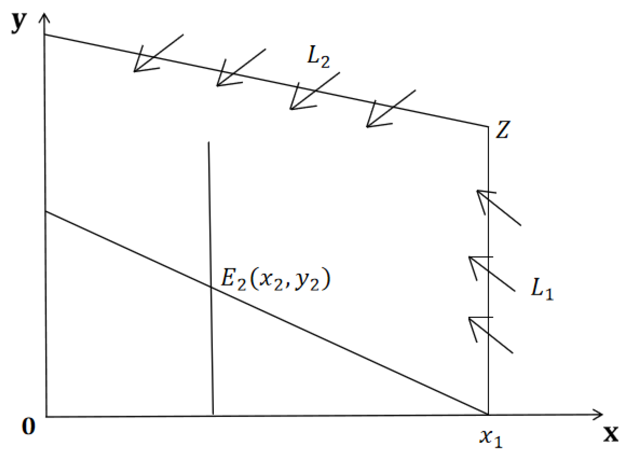
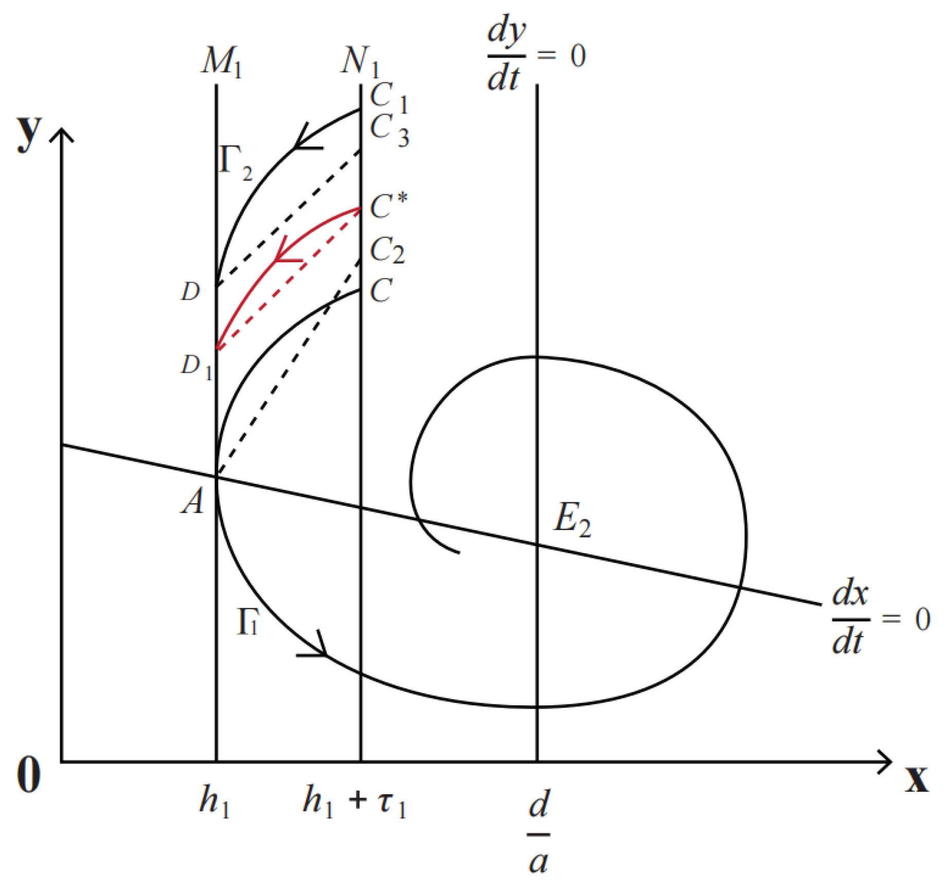
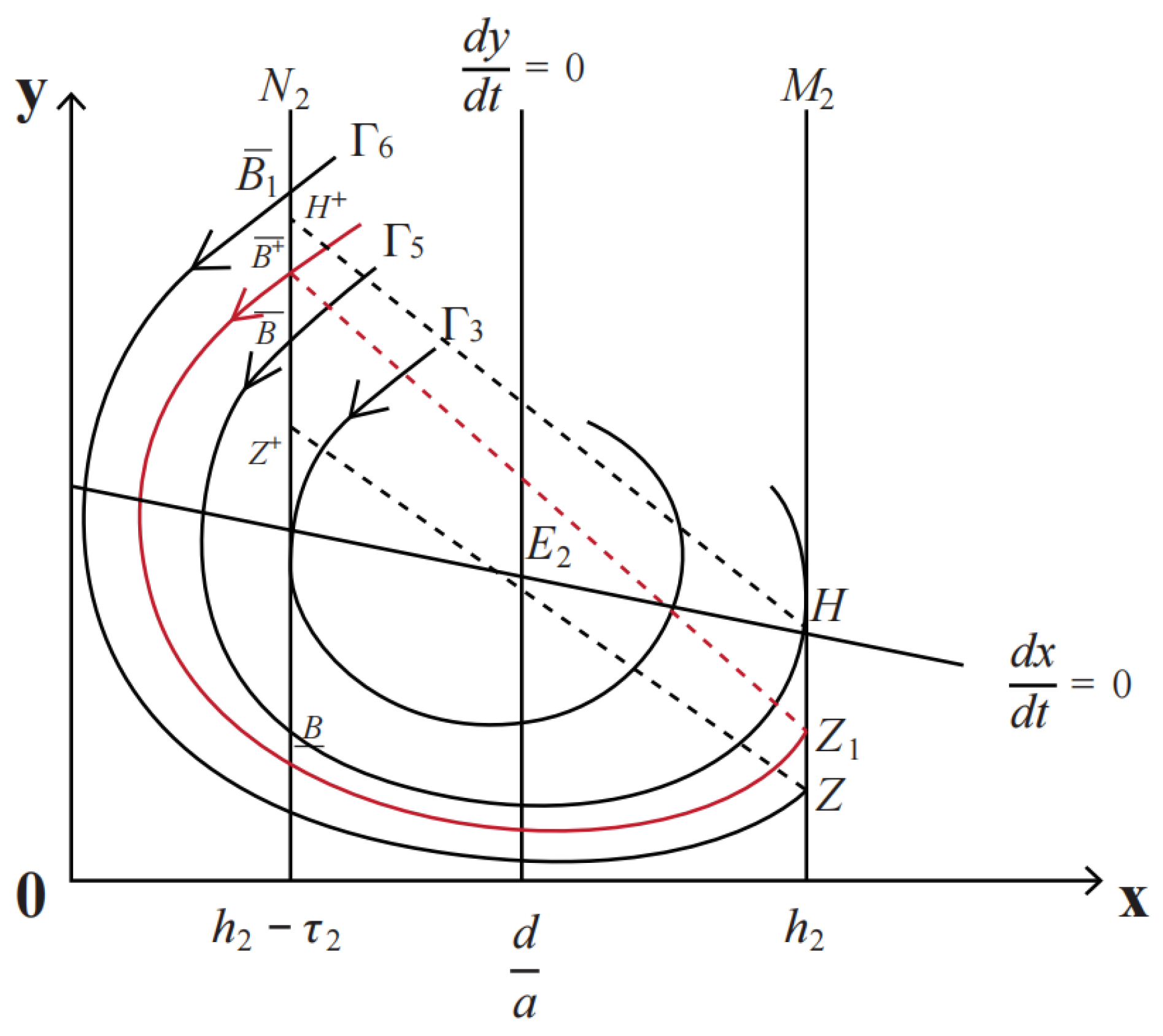
4.1. Existence and Stability of Order-1 Periodic Solution

First, we consider the system with one state-dependent impulse control.

$$\left\{\begin{array}{c}\left\{\begin{array}{c}{\displaystyle \frac{dx}{dt}}=rx\left(1-{\displaystyle \frac{x}{K}}\right)-Ex-bxy,\hfill \\ {\displaystyle \frac{dy}{dt}}=axy-dy,\hfill \end{array}\right\}x>h_1,\hfill \\ \left\{\begin{array}{c}\Delta x={\tau }_1,\hfill \\ \Delta y=-{\beta }_{1}y+\tau ,\hfill \end{array}\right\}x=h_1,\hfill \end{array}\right.$$

(7)

Let $x\left(t\right)$, $y\left(t\right)$ be a solution of system (1), defining the pulse set $M_1=\{(x\left(t\right),y\left(t\right))\in {\mathbb{R}}_{+}^2|x=h_1,y>0\}$, the phase set $N_1=\{(x\left(t\right),y\left(t\right))\in {\mathbb{R}}_{+}^2|x=h_1+{\tau }_1,y>0\}$, and the impulse function $I_1:(h_1,y)\in M_1\to (h_1+{\tau }_1,(1-{\beta }_1)y+\tau )\in N_1$. In order to facilitate the discussion, it is necessary to define the following.

The point $A(h_1,y_A)(y_A={\displaystyle \frac{1}{b}}[r(1-{\displaystyle \frac{h_1}{K}})-E])$ is the intersection of the pulse set $M_1$ with the ${\displaystyle \frac{dx}{dt}}=0$. From the qualitative theory of differential equations, it follows that there exists a unique trajectory ${\mathsf{\Gamma }}_1$ tangent to the pulse set at point A. When the trajectory ${\mathsf{\Gamma }}_1$ is tangent to the pulse set $M_1$ at the point A, crossing $N_1$ at $C(h_1+{\tau }_1,y_c)$.

Theorem 6. 

When ${\tau }_1>{\displaystyle \frac{d}{a}}-h_1$ and $\tau >y_C-(1-{\beta }_1)y_A$, the system (6) has an order-1 periodic solution.

Proof. 

As shown in Figure 3, the trajectory ${\mathsf{\Gamma }}_1$ is tangent to the pulse set $M_1$ at point $A(h_1,y_A)$, crossing at point $C(h_1+{\tau }_1,y_C)$. Then, the impulse function $I_1$ maps A to $C_2(x_{C_2},y_{C_2})$. If $\tau >y_C-(1-{\beta }_1)y_A$, the $C_2$ is above at C. We can conclude the successor function of point $C(h_1+{\tau }_1,y_C)$, $G\left(C\right)=y_{C_2}-y_C>0$.

Figure 3. System (6) has an order-1 periodic solution.

On the other hand, select the point $C_1(x_{C_1},y_{C_1})$, satisfying $y_{C_1}⋙0$. The orbit ${\mathsf{\Gamma }}_2$ starts from $C_1$ and crosses $M_1$ at the point D. Then, the impulse function will map it to the corresponding phase point $C_3(x_{C_3},y_{C_3})$. It is obvious that if $y_{C_3}<y_{C_1}$, we have $G\left(C_1\right)=y_{C_3}-y_{C_1}<0$.

So, there is a point $C*$ between $C_1$ and C satisfying $G\left(C*\right)=0$, and the system has an order-1 periodic solution. □

Theorem 7. 

The order-1 periodic solution of system (6) is orbital asymptotically stable over the initial point $(h_1,{\phi }_0)$.

Proof. 

Let

$$\begin{array}{cc}\hfill P(x,y)& =rx(1-{\displaystyle \frac{x}{K}})-Ex-bxy,Q(x,y)=axy-dy;\hfill \\ \hfill \Delta x& =A(x,y)={\tau }_1,\Delta y=B(x,y)=-{\beta }_{1}y+\tau ,\mathsf{\Phi }(x,y)=x-h_1=0;\hfill \\ \hfill \left(x\right(t),y(t\left)\right)& =(h_1,{\phi }_0),(x\left(t^{+}\right),y\left(t^{+}\right))=(h_1+{\tau }_1,(1-{\beta }_1){\phi }_0+\tau );\hfill \end{array}$$

$$\begin{array}{cc}\hfill {\displaystyle \frac{𝜕P}{𝜕x}}& =r-{\displaystyle \frac{2r}{K}}-E-by,{\displaystyle \frac{𝜕Q}{𝜕y}}=ax-d,{\displaystyle \frac{𝜕A}{𝜕x}}=0,{\displaystyle \frac{𝜕A}{𝜕y}}=0,\hfill \\ \hfill {\displaystyle \frac{𝜕B}{𝜕x}}& =0,{\displaystyle \frac{𝜕B}{𝜕y}}=-{\beta }_1,{\displaystyle \frac{𝜕\mathsf{\Phi }}{𝜕x}}=1,{\displaystyle \frac{𝜕\mathsf{\Phi }}{𝜕y}}=0;\hfill \\ \hfill {\Delta }_1& ={\displaystyle \frac{P_{+}(\frac{𝜕B}{𝜕y}\frac{𝜕\mathsf{\Phi }}{𝜕x}-\frac{𝜕B}{𝜕x}\frac{𝜕\mathsf{\Phi }}{𝜕y}+\frac{𝜕\mathsf{\Phi }}{𝜕x})+Q_{+}(\frac{𝜕A}{𝜕x}\frac{𝜕\mathsf{\Phi }}{𝜕y}-\frac{𝜕A}{𝜕y}\frac{𝜕\mathsf{\Phi }}{𝜕x}+\frac{𝜕\mathsf{\Phi }}{𝜕y})}{P\left(\frac{𝜕\mathsf{\Phi }}{𝜕x}\right)+Q\left(\frac{𝜕\mathsf{\Phi }}{𝜕y}\right)}}\hfill \\ & ={\displaystyle \frac{(1-{\beta }_1)P_{+}}{P}};\hfill \\ \hfill {\int }_0^T({\displaystyle \frac{𝜕P}{𝜕x}}+{\displaystyle \frac{𝜕Q}{𝜕y}})\mathrm{d}t& ={\int }_0^T(r-{\displaystyle \frac{2r}{K}}-E-by+ax-d)\mathrm{d}t;\hfill \\ \hfill {\int }_0^T(r-{\displaystyle \frac{r}{K}}-E-by)\mathrm{d}t& ={\int }_0^T{\displaystyle \frac{dx}{x}}={\int }_{h_1}^{h_1+{\tau }_1}{\displaystyle \frac{dx}{x}}=ln{\displaystyle \frac{h_1+{\tau }_1}{h_1}};\hfill \end{array}$$

$$\begin{array}{cc}\hfill {\int }_0^T(ax-d)\mathrm{d}t& ={\int }_0^T{\displaystyle \frac{dy}{y}}=ln{\displaystyle \frac{{\phi }_0}{(1-{\beta }_1){\phi }_0+\tau }};\hfill \\ \hfill {\mu }_2& ={\Delta }_{1}exp(ln{\displaystyle \frac{h_1+{\tau }_1}{h_1}}+ln{\displaystyle \frac{{\phi }_0}{(1-{\beta }_1){\phi }_0+\tau }}+{\int }_0^T(-{\displaystyle \frac{r}{K}}x)\mathrm{d}t)\hfill \\ \hfill & ={\Delta }_1{\displaystyle \frac{{\phi }_0(h_1+{\tau }_1)}{h_1[(1-{\beta }_1){\phi }_0+\tau ]}}exp[{\int }_0^T(-{\displaystyle \frac{r}{K}}x)\mathrm{d}t]\hfill \\ \hfill & ={\displaystyle \frac{(1-{\beta }_1)(h_1+{\tau }_1){\phi }_0{P}_{+}}{h_1[(1-{\beta }_1){\phi }_0+\tau ]}}exp[{\int }_0^T(-{\displaystyle \frac{r}{K}}x)\mathrm{d}t]\hfill \\ \hfill & =|1-{\displaystyle \frac{h_1[(1-{\beta }_1){\phi }_0+\tau -(1-{\beta }_1)(h_1+{\tau }_1){\phi }_0{P}_{+}}{h_1[(1-{\beta }_1){\phi }_0+\tau }}|exp[{\int }_0^T(-{\displaystyle \frac{r}{K}}x)\mathrm{d}t].\hfill \end{array}$$

Since $h_1[(1-{\beta }_1){\phi }_0+\tau ]-(1-{\beta }_1)(h_1+{\tau }_1)-h_1\left[(1-{\beta }_1){\phi }_0\right]<0$ and ${\int }_0^T(-{\displaystyle \frac{r}{K}}x)\mathrm{d}t<0$, the order-1 periodic solution of system (6) is orbital asymptotically stable over the initial point $(h_1,{\phi }_0)$. □

Then, we consider another system with one state-dependent impulse control.

$$\left\{\begin{array}{c}\left\{\begin{array}{c}{\displaystyle \frac{dx}{dt}}=rx\left(1-{\displaystyle \frac{x}{K}}\right)-Ex-bxy,\hfill \\ {\displaystyle \frac{dy}{dt}}=axy-dy,\hfill \end{array}\right\}x<h_2,\hfill \\ \left\{\begin{array}{c}\Delta x=-{\tau }_2,\hfill \\ \Delta y={\beta }_{2}y,\hfill \end{array}\right\}x=h_2.\hfill \end{array}\right.$$

(8)

Let $\left(x\right(t),y(t\left)\right)$ be a solution of the system, the pulse set $M_2=\{(x\left(t\right),y\left(t\right))\in {\mathbb{R}}_{+}^2|x=h_2,y>0\}$, the phase set $N_2=\{(x\left(t\right),y\left(t\right))\in {\mathbb{R}}_{+}^2|x=h_2-{\tau }_2,y>0\}$, and the impulse function $I_2:(h_2,y)\in M_2\to ((h_2-{\tau }_2),(1+{\beta }_2)y)\in N_2$. We denoted the point $H(h_2,y_H)(y_H={\displaystyle \frac{1}{b}}[r(1-{\displaystyle \frac{h_2}{K}})-E])$ as the intersection of pulse set $M_2$ with ${\displaystyle \frac{dx}{dt}}=0$; $Q(h_2-{\tau }_2,y_Q)$ is the intersection of phase set $N_2$ with ${\displaystyle \frac{dx}{dt}}=0$. There exists a unique trajectory ${\mathsf{\Gamma }}_3$ tangential to the phase set at point Q.

Case I. If the trajectory ${\mathsf{\Gamma }}_3$ is just through the point H.

Case II. If the trajectory ${\mathsf{\Gamma }}_3$ and $M_2$ do not have a crossing point, we denoted a trajectory ${\mathsf{\Gamma }}_4$, which is tangential to the $M_2$ at point $\overline{B}(x_{\overline{B}},y_{\overline{B}})$ and $\underline{B}(x_{\underline{B}},y_{\underline{B}})$

Theorem 8. 

For the Case I, if ${\tau }_2>max\{h_2-{\displaystyle \frac{d}{a}},{\displaystyle \frac{{\beta }_{2}KE}{r}}+{\beta }_2(K-h_2)\}$, the system (7) has an order-1 periodic solution.

Proof. 

As shown in Figure 4, when ${\tau }_2>h_2-{\displaystyle \frac{d}{a}}$, select point H, then the impulse function maps H to $Q_1(h_2-{\tau }_2,(1+{\beta }_2)y_H)$. If ${\tau }_2>{\displaystyle \frac{{\beta }_{2}KE}{r}}+{\beta }_2(K-h_2)>0$ is satisfied, then point $Q_1$ is below point Q. Thus, the successor function of point Q is $G\left(Q\right)=y_{Q_1}-y_Q<0$.

Figure 4. System (7) has an order-1 periodic solution.

On the other hand, choose another point $Q_2$ in the phase set $N_2$ that is sufficiently close to the x axis, and its coordinate is denoted as $Q_2(h_2-{\tau }_2,\epsilon )$, where $\epsilon$ is an arbitrarily small positive number. Under the control of the continuous map of system (7), the track initiating from $Q_2$ will reach the pulse set at $H_1$, then the impulsive function maps $H_1$ to $Q_3(h_2-{\tau }_2,(1+{\beta }_2)y_{H_1})$. Since $\epsilon$ is arbitrarily small, we can conclude that in the successor function of $Q_2$, $G\left(Q_2\right)=y_{Q_3}-y_{Q_2}>0$, there exists a point $Q^{*}$ between $Q_2$ and Q satisfying $G\left(Q*\right)=0$, so the system has an order-1 periodic solution. □

Theorem 9. 

For the CaseII, if $y_{\overline{B}}<{\displaystyle \frac{(1+{\beta }_2)}{b}}[r(1-{\displaystyle \frac{h_2}{K}})-E]$, the system has an order-1 periodic solution.

Proof. 

As shown in Figure 5, if ${\mathsf{\Gamma }}_3$ and $M_2$ do not have crossing points, the trajectory ${\mathsf{\Gamma }}_4$ with $M_2$ is tangential to the $H(h_2,{\displaystyle \frac{1}{b}}[r(1-{\displaystyle \frac{h_2}{K}})-E])$ and has two points crossing the $N_2$, denoted by $\overline{B}(x_{\overline{B}},y_{\overline{B}})$, $\underline{B}(x_{\underline{B}},y_{\underline{B}})$, respectively. The impulse function will map H to the corresponding phase point $H^{+}(h_2-{\tau }_2,{\displaystyle \frac{(1+{\beta }_2)}{b}}[r(1-{\displaystyle \frac{h_2}{K}})-E])$. If $y_{\overline{B}}<{\displaystyle \frac{(1+{\beta }_2)}{b}}[r(1-{\displaystyle \frac{h_2}{K}})-E]$, the point $H^{+}$ is above $\overline{B}$. So the successor function of point $\overline{B}$ is $G\left(\overline{B}\right)=y_{H^{+}}-y_{\overline{B}}>0$.

Figure 5. System (7) has an order-1 periodic solution.

On the other hand, there exists another point $\overline{B_1}$, satisfying $y_{\overline{B_1}}⋙0$, the trajectory ${\mathsf{\Gamma }}_5$ through it crossing the pulse sets $M_2$ at point Z. We can then get the successor function $G\left(\overline{B_1}\right)=y_{Z^{+}}-y_{\overline{B_1}}<0$. So there exists a point $\overline{B^{*}}$ between $\overline{B_1}$ and $\overline{B}$ where $G\left(\overline{B*}\right)=0$, and the system has an order-1 periodic solution. □

Theorem 10. 

The order-1 periodic solution of system (7) is orbital asymptotically stable over the initial point $(h_2,{\phi }_1)$.

Proof. 

Let

$$\begin{array}{cc}\hfill P(x,y)& =rx(1-{\displaystyle \frac{x}{K}})-Ex-bxy,Q(x,y)=axy-dy;\hfill \\ \hfill \Delta x=C(x,y)& =-{\tau }_2,\Delta y=D(x,y)={\beta }_{2}y,\mathsf{\Phi }(x,y)=x-h_2=0;\hfill \\ \hfill \left(x\right(t),y(t\left)\right)& =(h_2,{\phi }_1),(x\left(t^{+}\right),y\left(t^{+}\right))=(h_2-{\tau }_2,(1+{\beta }_2){\phi }_1);\hfill \\ \hfill {\displaystyle \frac{𝜕P}{𝜕x}}& =r-{\displaystyle \frac{2r}{K}}-E-by,{\displaystyle \frac{𝜕Q}{𝜕y}}=ax-d;\hfill \\ \hfill {\displaystyle \frac{𝜕C}{𝜕x}}& =0,{\displaystyle \frac{𝜕C}{𝜕y}}=0,{\displaystyle \frac{𝜕D}{𝜕x}}=0,{\displaystyle \frac{𝜕D}{𝜕y}}={\beta }_2,{\displaystyle \frac{𝜕{\mathsf{\Phi }}_1}{𝜕x}}=1,{\displaystyle \frac{𝜕{\mathsf{\Phi }}_1}{𝜕y}}=0;\hfill \\ \hfill {\Delta }_1& ={\displaystyle \frac{P_{+}(\frac{𝜕D}{𝜕y}\frac{𝜕{\mathsf{\Phi }}_1}{𝜕x}-\frac{𝜕D}{𝜕x}\frac{𝜕{\mathsf{\Phi }}_1}{𝜕y}+\frac{𝜕{\mathsf{\Phi }}_1}{𝜕x})+Q_{+}(\frac{𝜕C}{𝜕x}\frac{𝜕{\mathsf{\Phi }}_1}{𝜕y}-\frac{𝜕C}{𝜕y}\frac{𝜕{\mathsf{\Phi }}_1}{𝜕x}+\frac{𝜕{\mathsf{\Phi }}_1}{𝜕y})}{P\left(\frac{𝜕{\mathsf{\Phi }}_1}{𝜕x}\right)+Q\left(\frac{𝜕\mathsf{\Phi }}{𝜕y}\right)}}\hfill \\ & ={\displaystyle \frac{(1+{\beta }_2)P_{+}}{P}};\hfill \\ \hfill {\int }_0^T({\displaystyle \frac{𝜕P}{𝜕x}}+{\displaystyle \frac{𝜕Q}{𝜕y}})\mathrm{d}t& ={\int }_0^T(r-{\displaystyle \frac{2r}{K}}-E-by+ax-d)\mathrm{d}t;\hfill \\ \hfill {\int }_0^T(r-{\displaystyle \frac{r}{K}}-E-by)\mathrm{d}t& ={\int }_0^T{\displaystyle \frac{dx}{x}}={\int }_{h_2}^{h_2-{\tau }_2}{\displaystyle \frac{dx}{x}}=ln{\displaystyle \frac{h_2}{h_2-{\tau }_2}};\hfill \\ \hfill {\int }_0^T(ax-d)\mathrm{d}t& ={\int }_0^T{\displaystyle \frac{dy}{y}}=ln{\displaystyle \frac{1}{1+{\beta }_2}};\hfill \\ \hfill {\mu }_2& ={\Delta }_{1}exp(ln{\displaystyle \frac{h_2}{h_2-{\tau }_2}}+ln{\displaystyle \frac{1}{1+{\beta }_2}}+{\int }_0^T(-{\displaystyle \frac{r}{K}}x)\mathrm{d}t)\hfill \\ \hfill & ={\Delta }_1{\displaystyle \frac{h_2}{(1+{\beta }_2)(h_2-{\tau }_2)}}exp\left[{\int }_0^T(-{\displaystyle \frac{r}{K}}x)\mathrm{d}t\right]\hfill \\ \hfill & ={\displaystyle \frac{h_2{P}_{+}}{(h_2-{\tau }_2)P}}exp\left[{\int }_0^T(-{\displaystyle \frac{r}{K}}x)\mathrm{d}t\right]\hfill \\ \hfill & =|1-{\displaystyle \frac{(h_2-{\tau }_2)P-h_2{P}_{+}}{(h_2-{\tau }_2)P}}|exp\left[{\int }_0^T(-{\displaystyle \frac{r}{K}}x)\mathrm{d}t\right].\hfill \end{array}$$

Because $(h_2-{\tau }_2)P-h_2{P}_{+}-(h_2-{\tau }_2)P<0$ and ${\int }_0^T(-{\displaystyle \frac{r}{K}}x)\mathrm{d}t<0$, the order-1 periodic solution of system (7) is orbital asymptotically stable over the initial point $(h_2,{\phi }_1)$. □

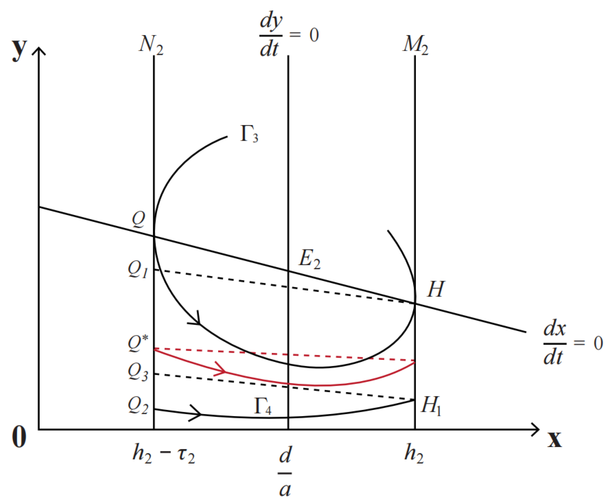
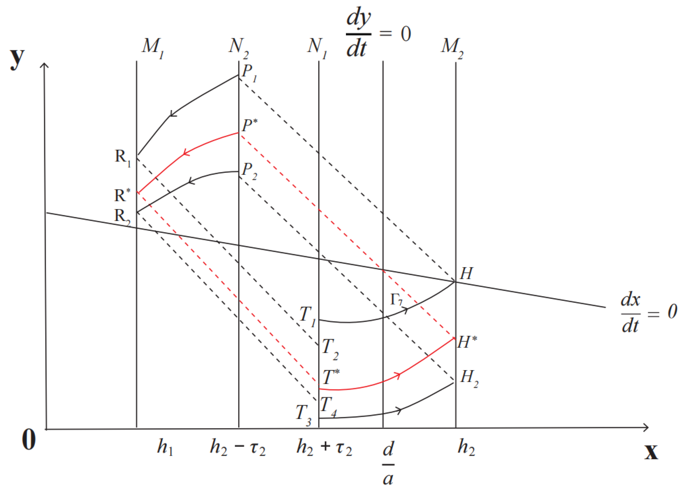
4.2. Existence and Stability of Order-2 Periodic Solution

First, we denoted a special trajectory ${\mathsf{\Gamma }}_7$, which from the initial point $T(h_1+\tau ,y_T)\in N_1$ is just tangential to the point H.

Theorem 11. 

If $h_1+{\tau }_1>h_2-{\tau }_2$ and $0<\tau <y_T-{\displaystyle \frac{(1-{\beta }_1)}{b}}[r(1-{\displaystyle \frac{h_1}{K}})-E]$, the system (2) has an order-2 periodic solution.

Proof. 

As shown in Figure 6, existence of the trajectory from the point $T(h_1+\tau ,y_T)$ tangential to the point $H(x_H,y_H)$ in the pulse set $M_2$. After that, the impulse function maps H to the point $P_1(h_2-{\tau }_2,y_P)$ in phase $N_2$. Following that, the first equation of model (2) dominates the trail of the pulse set $M_1$, and they cross at $R_1(h_1,y_{R_1})$, then the impulse function will map it to the corresponding phase point $T_2(h_2+{\tau }_2,y_{T_2})$. If $0<\tau <y_{T_1}-{\displaystyle \frac{(1-{\beta }_1)}{b}}[r(1-{\displaystyle \frac{h_1}{K}})-E]$, then $y_{T_1}-[(1+{\beta }_2)y_{R_1}+\tau ]>0$. Thus, $y_{T_1}>y_{T_2}$, which means $G\left(T_1\right)=y_{T_2}-y_{T_1}<0$.

Figure 6. System (2) has an order-2 periodic solution.

On the other hand, there exists another point $T_3(x_{T_3},y_{T_3})$, satisfying $0<y_{T_3}⋘1$, which moves to $H_2\in M_2$ and is mapped to $P_2(x_{P_2},y_{P_2})$. Then, the impulsive model (2) administrates the trail developing upper left until reaching the impulse set $M_1$ at $R_2$ and finally arriving at the phase set $N_1$ at $T_4(x_{T_4},y_{T_4})$. We have $G\left(T_3\right)=y_{T_4}-y_{T_3}>0$. So there exists a point $T^{*}$ between $T_1$ and $T_3$ satisfying $G\left(T*\right)=0$, then the system has an order-2 periodic solution. □

Theorem 12. 

The order-2 periodic solution of system (2) is orbital asymptotically stable.

Proof. 

$$\begin{array}{cc}\hfill P(x,y)& =rx(1-{\displaystyle \frac{x}{K}})-Ex-bxy,Q(x,y)=axy-dy;\hfill \\ \hfill A(x,y)& ={\tau }_1,B(x,y)=-{\beta }_{1}y+\tau ,\mathsf{\Phi }(x,y)=x-h_1=0;\hfill \\ \hfill C(x,y)& =-{\tau }_2,D(x,y)={\beta }_{2}y,\mathsf{\Phi }(x,y)=x-h_2=0;\hfill \\ \hfill {\displaystyle \frac{𝜕P}{𝜕x}}& =r-{\displaystyle \frac{2r}{K}}-E-by,{\displaystyle \frac{𝜕Q}{𝜕y}}=ax-d;\hfill \\ \hfill {\displaystyle \frac{𝜕A}{𝜕x}}& =0,{\displaystyle \frac{𝜕A}{𝜕y}}=0,{\displaystyle \frac{𝜕B}{𝜕x}}=0,{\displaystyle \frac{𝜕B}{𝜕y}}=-{\beta }_1,{\displaystyle \frac{𝜕\mathsf{\Phi }}{𝜕x}}=1,{\displaystyle \frac{𝜕\mathsf{\Phi }}{𝜕y}}=0;\hfill \\ \hfill {\displaystyle \frac{𝜕C}{𝜕x}}& =0,{\displaystyle \frac{𝜕C}{𝜕y}}=0,{\displaystyle \frac{𝜕D}{𝜕x}}=0,{\displaystyle \frac{𝜕D}{𝜕y}}={\beta }_2,{\displaystyle \frac{𝜕{\mathsf{\Phi }}_1}{𝜕x}}=1,{\displaystyle \frac{𝜕{\mathsf{\Phi }}_1}{𝜕y}}=0;\hfill \\ \hfill {\Delta }_1& ={\displaystyle \frac{P_{+}(\frac{𝜕B}{𝜕y}\frac{𝜕\mathsf{\Phi }}{𝜕x}-\frac{𝜕B}{𝜕x}\frac{𝜕\mathsf{\Phi }}{𝜕y}+\frac{𝜕\mathsf{\Phi }}{𝜕x})+Q_{+}(\frac{𝜕A}{𝜕x}\frac{𝜕\mathsf{\Phi }}{𝜕y}-\frac{𝜕A}{𝜕y}\frac{𝜕\mathsf{\Phi }}{𝜕x}+\frac{𝜕\mathsf{\Phi }}{𝜕y})}{P\left(\frac{𝜕\mathsf{\Phi }}{𝜕x}\right)+Q\left(\frac{𝜕\mathsf{\Phi }}{𝜕y}\right)}}\hfill \\ \hfill & ={\displaystyle \frac{(1-{\beta }_1)P_{+}}{P}}={\displaystyle \frac{P\left(H^{*}\right)(1-{\beta }_1)}{P\left(R*\right)}};\hfill \\ \hfill {\Delta }_2& ={\displaystyle \frac{P_{+}(\frac{𝜕D}{𝜕y}\frac{𝜕{\mathsf{\Phi }}_1}{𝜕x}-\frac{𝜕D}{𝜕x}\frac{𝜕{\mathsf{\Phi }}_1}{𝜕y}+\frac{𝜕{\mathsf{\Phi }}_1}{𝜕x})+Q_{+}(\frac{𝜕C}{𝜕x}\frac{𝜕{\mathsf{\Phi }}_1}{𝜕y}-\frac{𝜕C}{𝜕y}\frac{𝜕{\mathsf{\Phi }}_1}{𝜕x}+\frac{𝜕{\mathsf{\Phi }}_1}{𝜕y})}{P\left(\frac{𝜕{\mathsf{\Phi }}_1}{𝜕x}\right)+Q\left(\frac{𝜕\mathsf{\Phi }}{𝜕y}\right)}}\hfill \\ \hfill & ={\displaystyle \frac{(1+{\beta }_2)P_{+}}{P}}={\displaystyle \frac{Q^{*}(1+{\beta }_2)}{P\left(R*\right)}};\hfill \\ \hfill {\int }_0^{T_1+T_2}({\displaystyle \frac{𝜕P}{𝜕x}}+{\displaystyle \frac{𝜕Q}{𝜕y}})\mathrm{d}t& ={\int }_0^{T_1}(r-{\displaystyle \frac{2r}{K}}-E-by+ax-d)\mathrm{d}t\hfill \\ & +{\int }_0^{T_2}(r-{\displaystyle \frac{2r}{K}}-E-by+ax-d)\mathrm{d}t;\hfill \\ & ={\int }_{h_1+{\tau }_1}^{h_1}{\displaystyle \frac{dx}{x}}\mathrm{d}t+{\int }_{y_{R*}}^{(1-{\beta }_1)y_{R*}+\tau }{\displaystyle \frac{dy}{y}}\mathrm{d}+{\int }_{h_2}^{h_2-{\tau }_2}{\displaystyle \frac{dx}{x}}\mathrm{d}t\hfill \\ \hfill & +{\int }_{y_{P*}}^{(1+{\beta }_2)y_{P*}+\tau }{\displaystyle \frac{dy}{y}}\mathrm{d}t+{\int }_0^{T_1+T_2}{\displaystyle \frac{dx}{x}}\mathrm{d}t;\hfill \\ \hfill {\mu }_2& ={\Delta }_1{\Delta }_{2}exp\left[{\int }_0^{T_1+T_2}({\displaystyle \frac{𝜕P}{𝜕x}}+{\displaystyle \frac{𝜕Q}{𝜕y}})\mathrm{d}t\right]\hfill \\ & ={\displaystyle \frac{P\left(H^{*}(1-{\beta }_1)h_1{h}_2{y}_{R*}\right)}{P\left(P*\right)P\left(R*\right)(h_1+{\tau }_1)[(1-{\beta }_1)y_{R*}+\tau ](h_2-{\tau }_2)}}\hfill \\ & =|1-{\displaystyle \frac{P(P*)P\left(R*\right)(h_1+{\tau }_1)[(1-{\beta }_1)y_{R^{*}}+\tau ](h_2-{\tau }_2)-P\left(H*(1-{\beta }_1)h_1{h}_2{y}_{R*}\right)}{P\left(P*\right)P\left(R*\right)(h_1+{\tau }_1)[(1-{\beta }_1)y_{R*}+\tau ](h_2-{\tau }_2)}}|\hfill \\ & \times exp\left[{\int }_0^{T_1+T_2}\left({\displaystyle \frac{-rx}{K}}\right)\mathrm{d}t\right].\hfill \end{array}$$

It is obvious that the order-2 periodic solution of system (2) is orbital asymptotically stable. □

5. Numerical Simulation

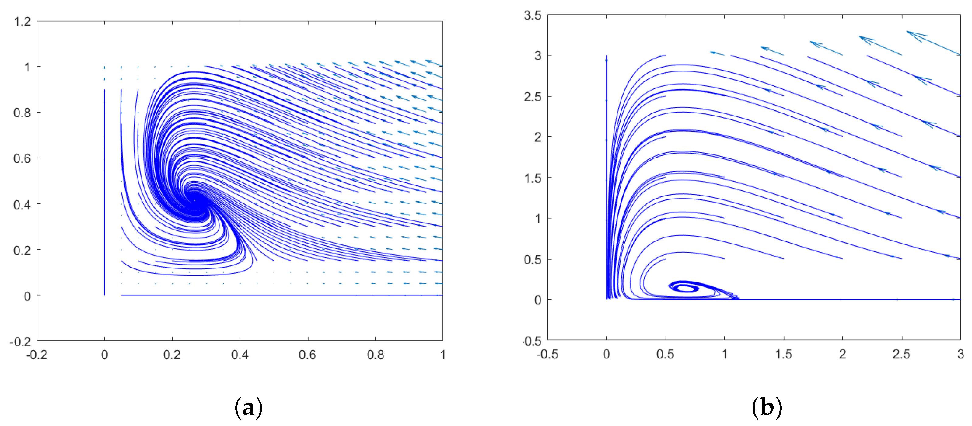
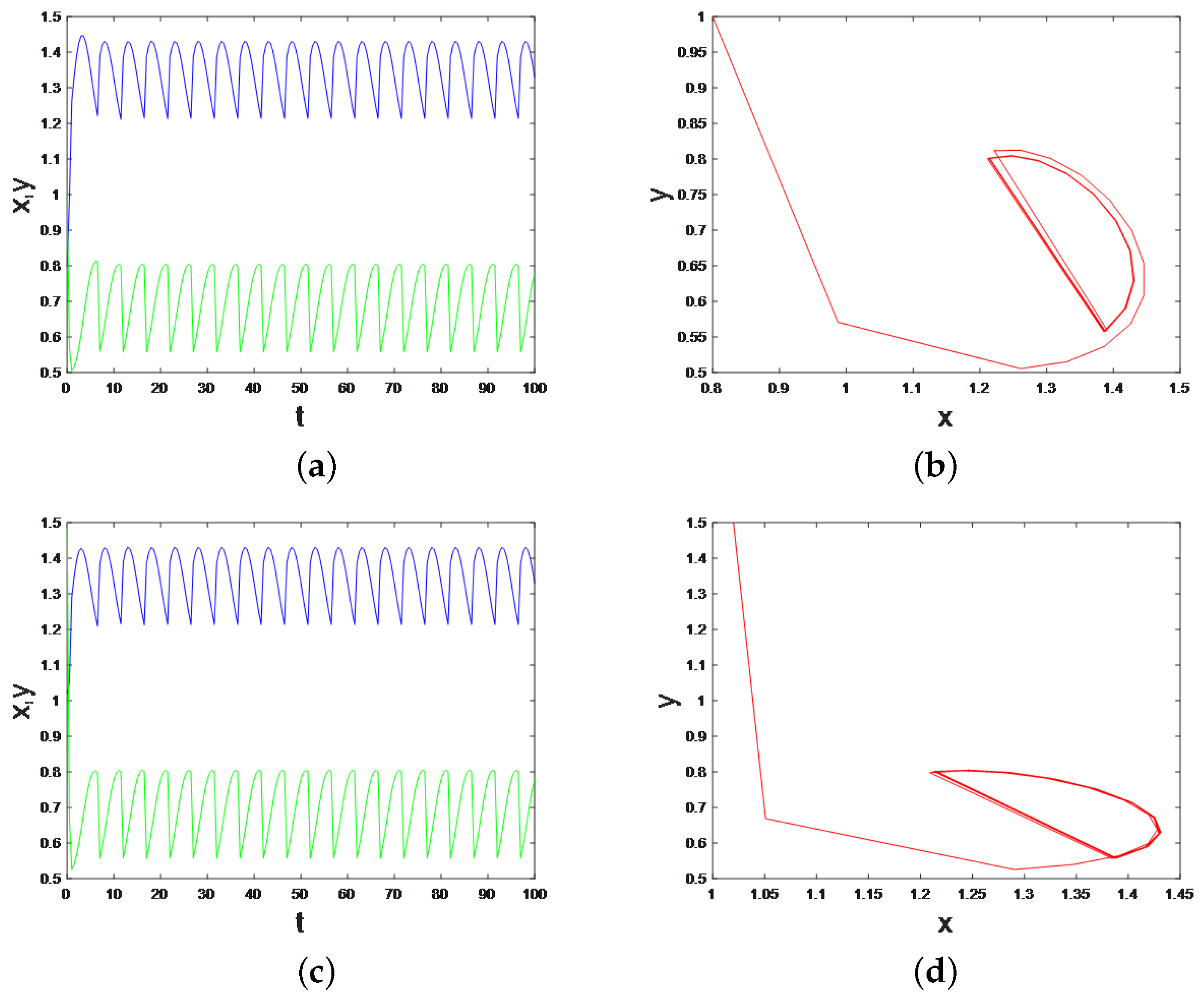
5.1. The Order-1 Periodic Solution Numerical Simulation

In the model (6), let $r=0.6,E=0.3,a=0.7,b=0.6,K=4.5,d=0.87,h_1=1.2,{\tau }_1=0.2,{\beta }_1=0.8,\tau =0.4$, then the model is defined as:

$$\left\{\begin{array}{c}\left\{\begin{array}{c}{\displaystyle \frac{dx}{dt}}=0.6x(1-{\displaystyle \frac{x}{4.5}})-0.3x-0.6xy,\hfill \\ {\displaystyle \frac{dy}{dt}}=0.7xy-0.87y,\hfill \end{array}\right\}x>1.2,\hfill \\ \left\{\begin{array}{c}\Delta x=0.2,\hfill \\ \Delta y=-0.8y+0.4,\hfill \end{array}\right\}x=1.2.\hfill \end{array}\right.$$

(9)

Theorem 6’s result indicates that the model has an order-1 periodic solution. Using Matlab for numerical simulation, we are able to obtain the dynamical trajectories, which are displayed in Figure 7. From the different initial values $x_0=1.02,y_0=1.5$ and $x_0=0.8,y_0=1$, the model has an order-1 periodic solution. If there is less algae, there is an ecological need to maintain balance by releasing algae and fishing fish.

Figure 7. Schematic representation of order-1 successor function and order-1 periodic solution. (a) The order-1 successor function from the initial point $(0.8,1)$. (b) The order-1 periodic solution from the initial point $(0.8,1)$. (c) The order-1 successor function from the initial point $(1.02,1.5)$. (d) The order-1 periodic solution from the initial point $(1.02,1.5)$.

The existence of the order-1 periodic solution means that putting in some food resources can maintain the water balance and fish cultivation. However, to keep the order-1 solution stable, we must control the amount of algae investment. For fish cultivation, the fish cannot have enough food, which presents an obstacle to its economic value.

In the model (7), let $r=0.6$, $E=0.3$, $a=0.25$, $K=4.8$, $d=0.68$, $h_2=2.39$, ${\tau }_2=0.6$, and ${\beta }_2=0.4$; the model is defined as

$$\left\{\begin{array}{c}\left\{\begin{array}{c}{\displaystyle \frac{dx}{dt}}=0.6x(1-{\displaystyle \frac{x}{4.8}})-0.3x-0.6xy,\hfill \\ {\displaystyle \frac{dy}{dt}}=0.25xy-0.68y,\hfill \end{array}\right\}x<2.39,\hfill \\ \left\{\begin{array}{c}\Delta x=-0.2,\hfill \\ \Delta y=0.4y,\hfill \end{array}\right\}x=2.39,\hfill \end{array}\right.$$

(10)

Theorem 8’s result indicates that the model has an order-1 periodic solution. Using Matlab for numerical simulation, we are able to obtain the dynamical trajectories, which are displayed in Figure 8. From the different initial values $x_0=0.8$, $y_0=1$, and $x_0=1.6$, $y_0=1.1$, the model has an order-1 periodic solution. If there is excessive algae, there is an ecological need to maintain balance by fishing algae and releasing fish. Theorem 9 is similar to Theorem 8, so we do not analyze it here.

Figure 8. Schematic representation of order-1 successor function and order-1 periodic solution. (a) The order-1 successor function from the initial point $(0.8,1)$. (b) The order-1 periodic solution from the initial point $(0.8,1)$. (c) The order-1 successor function from the initial point $(1.6,1.1)$. (d) The order-1 periodic solution from the initial point $(1.6,1.1)$.

The existence of the order-1 periodic solution means that investing fish and eliminating algae can keep the dynamics balanced. However, it cannot be used to consider fish harvesting.

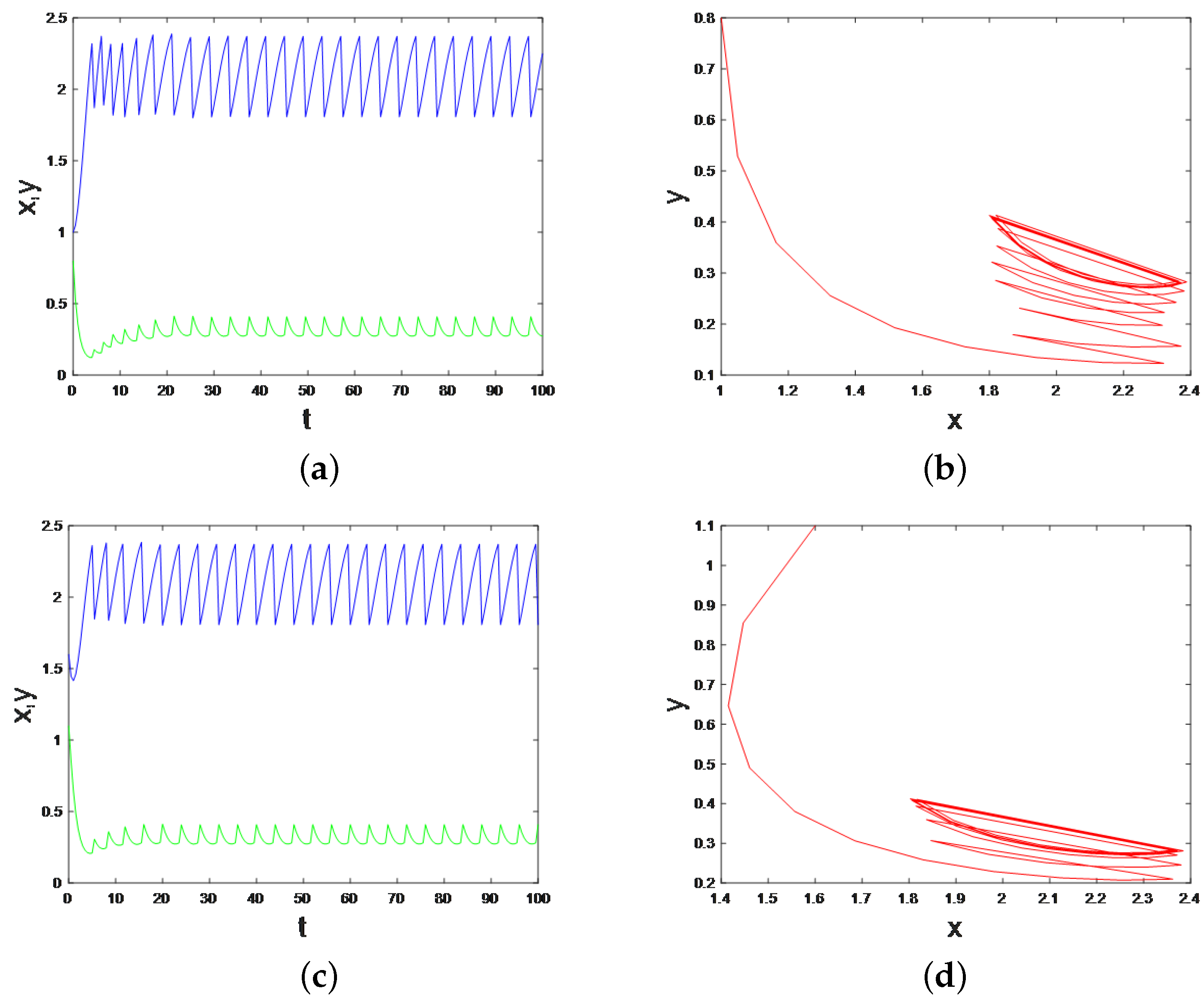
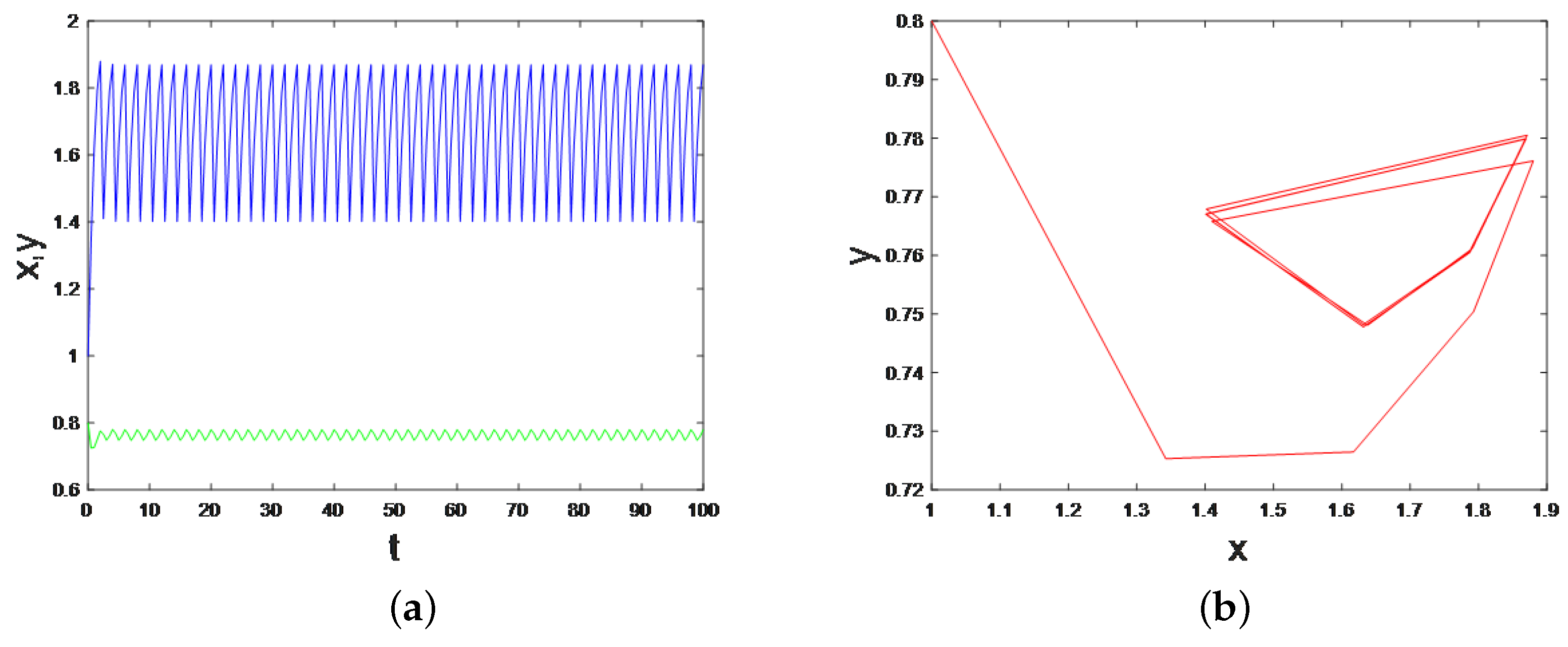
5.2. The Order-2 Periodic Solution Numerical Simulation

Let $r=0.6$, $E=0.3$, $a=0.66$, $b=0.7$, $K=4.5$, $d=0.8$, $h_1=1.4$, ${\tau }_1=1.2$, ${\beta }_1=0.65$, $\tau =0.3$, $h_2=3$, ${\tau }_2=0.7$, ${\beta }_2=0.38$, then the model is defined as

$$\left\{\begin{array}{c}\left\{\begin{array}{c}{\displaystyle \frac{dx}{dt}}=0.6x\left(1-{\displaystyle \frac{x}{4.5}}\right)-0.3x-0.7xy,\hfill \\ {\displaystyle \frac{dy}{dt}}=0.66xy-0.8y,\hfill \end{array}\right\}1.4<x<3.7,\hfill \\ \left\{\begin{array}{c}\Delta x=1.2,\hfill \\ \Delta y=-0.65y+0.3,\hfill \end{array}\right\}x=1.4,\hfill \\ \left\{\begin{array}{c}\Delta x=-0.7,\hfill \\ \Delta y=0.4y,\hfill \end{array}\right\}x=3.7,\hfill \end{array}\right.$$

(11)

By Theorem 11, the model possesses an order-2 periodic solution. According to the numerical simulation by Matlab, we can get the dynamical trajectories as shown in Figure 9. This means that the model with two impulses can maintain the ecological balance when the number of algae is too high or too low. In other words, the bilateral state-feedback pulse model can be used to maintain the ecological balance between algae and fish in the pond. When the algae’s population size is greater than the threshold, it can be prevented and controlled by fishing algae and releasing fish. On the contrary, if the algae populations are too small, the algae population can be increased, and the fish population can be decreased to maintain the ecological balance.

Figure 9. Schematic representation of order-2 successor function and order-2 periodic solution. (a) The order-2 successor function. (b) The order-2 periodic solution.

6. Conclusions

In this paper, we establish a class of algae–fish ecological models with two state-dependent impulses and investigate the existence of order-1 and order-2 periodic solutions within the system. Using the successor function and the geometric theory of semi-continuous dynamical systems, we prove the orbital asymptotic stability of these solutions. Numerical simulations further confirm the existence of order-1 and order-2 periodic solutions. A comparison between the two models demonstrates that the double-pulse model is more effective than the single-pulse model. In terms of algae control and aquaculture, the system with two impulses offers a significant approach to managing algae populations. This method not only allows for scientific and environmentally friendly algae control but also enhances the benefits of aquaculture.

This paper primarily focuses on a detailed analysis of the stability of order-1 and order-2 periodic solutions in the models. There are still many aspects that require further investigation. For instance, obtaining population data with practical significance would enrich the results of numerical simulations. Additionally, the stability of the system under diffusion conditions could also be considered.

References

- Srirengaraj, V.; Einar, R.; Hamed, G. Use of Algae in Aquaculture: A Review. Fishes 2024, 9, 63. [Google Scholar] [CrossRef]
- Wang, C.; Jiang, C.; Gao, T. Improvement of fish production and water quality in a recirculating aquaculture pond enhanced with bacteria-microalgae association. Aquaculture 2022, 547, 737420. [Google Scholar] [CrossRef]
- Chen, L. Mathematical Ecology Model and Research Method; Science Press: Beijing, China, 2017; pp. 259–318. [Google Scholar]
- Tang, S.; Xiao, Y. Biomathematics; Science Press: Beijing, China, 2019; pp. 132–168. [Google Scholar]
- Chen, L. Pest management and geometric theory of semicontinuous dynamical systems. Beihua Univ. (Nat. Sci.) 2011, 12, 1–9. [Google Scholar]
- Gazi, N.; Das, K. Structural stability analysis of an algal bloom mathematical model in tropic interaction. Nonlinear Anal. Real World Appl. 2010, 11, 2191–2206. [Google Scholar] [CrossRef]
- Yoshioka, H.; Yaegashi, Y. Singular stochastic control model for algae growth management in dam downstream. J. Biol. Dyn. 2018, 12, 242–270. [Google Scholar] [CrossRef] [PubMed]
- Fu, J.; Chen, L. Feedback control of water hyacinth ecosystem state. Appl. Math. 2013, 26, 51–57. [Google Scholar]
- Zhao, C.; Chen, L. The geometrical analysis of a predator-pery model with two state impulses. Math. Biosci. 2012, 238, 55–64. [Google Scholar] [CrossRef] [PubMed]
- Fu, J.; Chen, L. Modelling and qualitative analysis of water hyacinth ecological system with two state-dependent impulse controls. Complexity 2018, 2018, 4543976. [Google Scholar] [CrossRef]
- Zhou, M. Dynamics Analysis of Competing Systems with State Feedback Control; Xinyang Normal University: Xinyang, China, 2022. [Google Scholar]
- Zhang, M.; Zhao, Y. State feedback impulsive modeling and dynamic analysis of ecological balance in aquaculture water with nutritional utilization rate. Appl. Math. Comput. 2020, 373, 125007. [Google Scholar] [CrossRef]
Disclaimer/Publisher’s Note: The statements, opinions and data contained in all publications are solely those of the individual author(s) and contributor(s) and not of MDPI and/or the editor(s). MDPI and/or the editor(s) disclaim responsibility for any injury to people or property resulting from any ideas, methods, instructions or products referred to in the content. |
© 2024 by the authors. Licensee MDPI, Basel, Switzerland. This article is an open access article distributed under the terms and conditions of the Creative Commons Attribution (CC BY) license (https://creativecommons.org/licenses/by/4.0/).