Some Novel Fusion and Fission Phenomena for an Extended (2+1)-Dimensional Shallow Water Wave Equation

Abstract

An extended (2+1)-dimensional shallow water wave (SWW) model which can describe the evolution of nonlinear shallow water wave propagation in two spatial and temporal coordinates, is systematically studied. The multi-linear variable separation approach is addressed to the extended (2+1)-dimensional SWW equation. The variable separation solution consisting of two arbitrary functions is obtained, by assumption, from a specific ansatz. By selecting these two arbitrary functions as the exponential and trigonometric forms, resonant dromion, lump, and solitoff solutions are derived. Meanwhile, some novel fission and fusion phenomena including the semifoldons, peakons, lump, dromions, and periodic waves are studied with graphical and analytical methods. The results can be used to enhance the variety of the dynamics of the nonlinear wave fields related by engineering and mathematical physics.

1. Introduction

The study of integrable systems has developed into a mature theory because they reveal essential features in the diversity of engineering fields [1]. Many scholars have been seeking to expand and influence innovative techniques for solving integrable systems. Various effective methods have been presented to discuss and categorize the dynamical properties of the derived models [2,3,4,5,6,7,8,9,10]. The different types of nonlinear localized waves are often challenged by using traditional methods. An exact solution of the Liouville equation is given by introducing the variable separation from [11]. The multi-linear variable separation approach (MLVSA) for the higher-order dimensional nonlinear systems has been successfully established firstly to the Davey-Stewartsen equation [12] and confirmed in many nonlinear systems [13,14,15]. Numerous direct approaches based on various mapping equations such as the extended tanh function method, the enhanced projective approach, the projective Ricatti equation method and the q-deformed hyperbolic functions approach are selected to achieve the variable separation procedure [16,17,18,19,20,21,22,23]. The universal formula, in which exists the quite rich localized excitations, is revealed by means of the MLVSA. By selecting appropriate arbitrary functions of the universal formula, the rich exact solution including the interacting solutions can be obtained. Recently, the general variable separation solution including three independent functions is constructed based on another ansatz form [24]. A doubly periodic wave and a ring soliton, a four-humped dromion or lump, and a doubly periodic wave are obtained by using the general MLVSA.

On the other hand, an extended (2+1)-dimensional shallow water wave (SWW) equation is constructed based on the P-polynomials and the $D_{\overline{p}}$-operators. The extended (2+1)-dimensional SWW model reads as [25]

$$\begin{array}{c}\hfill u_{yt}+{\alpha }_1(3u_{xxxy}-3u_{xx}{u}_y-3u_x{u}_{xy})+{\alpha }_2{u}_{xy}=0,\end{array}$$

(1)

where ${\alpha }_1$ and ${\alpha }_2$ are free arbitrary constants. This nonlinear model in two spatial and temporal coordinates describes the development of nonlinear propagation shallow water waves. The phenomena of solitons and nonlinear waves for a Riemann wave moving along the y-axis and a long-wavelength propagating along the x-axis in fluid dynamics, plasma physics and almost non-dispersive media are widely studied for the SWW model [26]. The multiple lump and diverse varieties of interactions have been observed by the results obtained through numerical simulation [27]. The multi-kink solitons accompanied by the fission and fusion are presented by using the Hirota bilinear technique [28]. The fusion and fission phenomena consisting of semifoldons, peakons, lump, dromions and periodic waves for the extended (2+1)-dimensional SWW Equation (1) have been not discussed. In this paper, we consider the semifoldons’ fission and fusion phenomena, and lump, peakons, dromions and periodic wave fusion phenomena for the (2+1)-dimensional SWW equation by the MLVSA. One bell-like semifoldon divides into two bell-like semifoldons with a time evolution. Diverse types that are localized, such as two peakons and two dromions, as well as two peakons, one lump and one dromion will be fused to one dromion. Two peakons, one lump, one dromion and periodic waves merge together with one dromion and periodic waves by adding a periodic wave in an arbitrary function.

The remainder of this paper is arranged as follows. In Section 2, the solution with two arbitrary variable and separated functions of the SWW equation is constructed by a special variable separation approach. In Section 3, the resonant dromion, lump, and solitoff solutions are given by restricting the exponential forms as the arbitrary functions. The bright and dark dromion, different types of lump waves and solitoff solutions can be constructed by selecting appropriate parameters. Some novel solutions, such as semifoldon fission and fusion situations, lump, peakons, dromions and periodic wave fusion phenomena are given by restricting exponential and trigonometric forms in arbitrary functions. Other nonlinear excitations and interaction behaviors can be explored by selecting different types of arbitrary functions. Section 4 is dedicated to the discussion and conclusion.

2. Materials and Methods

In order to apply the MLVSA, the auto-Bäcklund transformation is introduced by the truncated Painlevé analysis

$$\begin{array}{c}\hfill u=\frac{u_0}{f}+u_1,\end{array}$$

(2)

where $f=f(x,y,t)$ is a function of the indicated variable. By substituting (2) into (1) and balancing the coefficient $f^{-5}$, we obtain the solution of $u_0$

$$\begin{array}{c}\hfill u_0=-2f_x.\end{array}$$

(3)

Here, $u_1=u_1(x,t)$ is the indeterminate seed solution of the equation. Replacing (2) into (1), the trilinear form reads as

$$\begin{array}{c}[{\alpha }_1{(3u_{1x}{f}_{xy}-f_{xxxy})}_x-{\alpha }_2{f}_{xxy}-f_{txy}]f^2+[{\left(f_x{f}_y\right)}_t+f_{xy}{f}_t-3{\alpha }_1{f}_y{\left(u_{1x}{f}_x\right)}_x\hfill \\ -6{\alpha }_1{u}_{1x}{f}_{xy}{f}_x+{\alpha }_1{f}_{xxxx}{f}_y+{\alpha }_2{f}_{xx}{f}_y+4{\alpha }_1{f}_x{f}_{xxxy}-2{\alpha }_1{f}_{xy}{f}_{xxx}+2{\alpha }_2{f}_x{f}_{xy}]f\hfill \\ +2f_x[3{\alpha }_1{u}_{1x}{f}_x{f}_y-{\alpha }_1{f}_y{f}_{xxx}-{\alpha }_2{f}_x{f}_y-3{\alpha }_1{f}_x{f}_{xxy}+3{\alpha }_1{f}_{xy}{f}_{xx}-f_y{f}_t]=0.\hfill \end{array}$$

(4)

The solution of (4) takes the following ansatz from

$$\begin{array}{c}\hfill f=a_0+a_{1}p+a_{2}q+a_{3}pq,\end{array}$$

(5)

where $a_0,a_1,a_2$ and $a_3$ are arbitrary constants; $p=p(x,t)$ and $q=q(y,t)$ are functions depending on the mentioned arguments. Replacing (5) into (4), one obtains

$$\begin{array}{c}\left(a_1+a_{3}q-\frac{f{\partial }_x}{2p_x}\right)(p_t+{\alpha }_1{p}_{xxx}+{\alpha }_2{p}_x)+(a_1+a_{3}q)(q_t-3{\alpha }_1{u}_{1x}{p}_x)\\ +\frac{3{\alpha }_{1}f}{2}(u_{1xx}+\frac{u_{1x}{p}_{xx}}{p_x})+(a_2+a_{3}p)q_t-f\frac{q_{ty}}{2q_y}=0.\end{array}$$

(6)

The equation mentioned above can be split into two separate equations. Two independent equations contain the functions as p and q, respectively

$$\begin{array}{cc}\hfill & p_t+{\alpha }_1{p}_{xxx}+{\alpha }_2{p}_x-3{\alpha }_1{u}_{1x}{p}_x-(a_0{a}_3-a_1{a}_2)[c_1\left(t\right)p^2+c_2\left(t\right)p+c_3\left(t\right)]=0,\end{array}$$

(7)

$$\begin{array}{cc}& q_t-c_1\left(t\right){(a_0+a_{2}q)}^2+c_2\left(t\right)(a_1+q{a}_3)(a_0+a_{2}q)-c_3\left(t\right){(a_1+a_{3}q)}^2=0,\end{array}$$

(8)

where $c_i,i=1,2,3$ are unrestricted functions of t. Due to $u_1$ and p being the arbitrary functions of x and t, we select the form of $u_1$ to identify (7). The function of $u_{1x}$ reads as

$$\begin{array}{c}\hfill u_{1x}=\frac{1}{3{\alpha }_1{p}_x}[p_t+{\alpha }_1{p}_{xxx}+{\alpha }_2{p}_x-(a_0{a}_3-a_1{a}_2)\left(c_1\left(t\right)p^2+c_2\left(t\right)p+c_3\left(t\right)\right)].\end{array}$$

(9)

As for (7), the general solution takes the type

$$\begin{array}{c}\hfill q=\frac{A_1\left(t\right)}{A_3\left(t\right)+F\left(y\right)}+A_2\left(t\right),\end{array}$$

(10)

where $F\left(y\right)$ is an unspecified function of the indicated variable and $A_i,(i=1,2,3)$ are arbitrary functions of t. By substituting (10) into (7), $A_1,A_2$ and $A_3$ are related to $c_1$, $c_2$ and $c_3$, as follows

$$\begin{array}{c}{c}_1\left(t\right)=\frac{1}{{(a_0{a}_3-a_1{a}_2)}^2}[a_3^2{A}_{2t}-a_3{A}_{1t}(a_3{A}_2+a_1)-A_{3t}{(a_3{A}_2+a_1)}^2],\\ c_2\left(t\right)=\frac{1}{{(a_0{a}_3-a_1{a}_2)}^2}[2a_2{a}_3{A}_{2t}-(2a_2{a}_3{A}_2+a_0{a}_3+a_1{a}_2)\frac{A_{1t}}{A_1}-2(A_2{a}_3+a_1)(a_2{A}_2+a_0)\frac{A_{3t}}{A_1},\\ c_3\left(t\right)=\frac{1}{{(a_0{a}_3-a_1{a}_2)}^2}[a_2^2{A}_{2t}-a_2(A_2{a}_2+a_0)\frac{A_{1t}}{A_1}-{(A_2{a}_2+a_0)}^2\frac{A_{3t}}{A_1}].\end{array}$$

(11)

By the above in detail calculations, a quite general solution of the SWW equation is

$$\begin{array}{c}\hfill u=u_1(x,t)-\frac{2p_x(q{a}_3+a_1)}{a_{3}pq+a_{1}p+a_{2}q+a_0},\end{array}$$

(12)

where p can take any form with respect to x and t, q is decided by (10) and $u_1$ is fixed by Equation (9).

MLVSA theorem. If p and q are solutions of arbitrary functions of $\{x,t\}$ and $\{y,t\}$, respectively, the universal formula is constructed as the following form by differentiating (12), with respect to y once

$$\begin{array}{c}\hfill w=u_y=\frac{2p_x{q}_y(a_0{a}_3-a_1{a}_2)}{{(a_{3}pq+a_{1}p+a_{2}q+a_0)}^2}.\end{array}$$

(13)

The expression of (13) was validated in some physical equation including the Darvey-Stewartson equation [13], the Broer-Kaup-Kupershmidt system [16], the asymmetric Nizhnik-Novikov-Veselov system [17] and so on [18,19,20,21]. We can obtain some types of specific solutions due to the flexibility of the functions p and q for the MLVSA theorem.

3. Results and Discussion

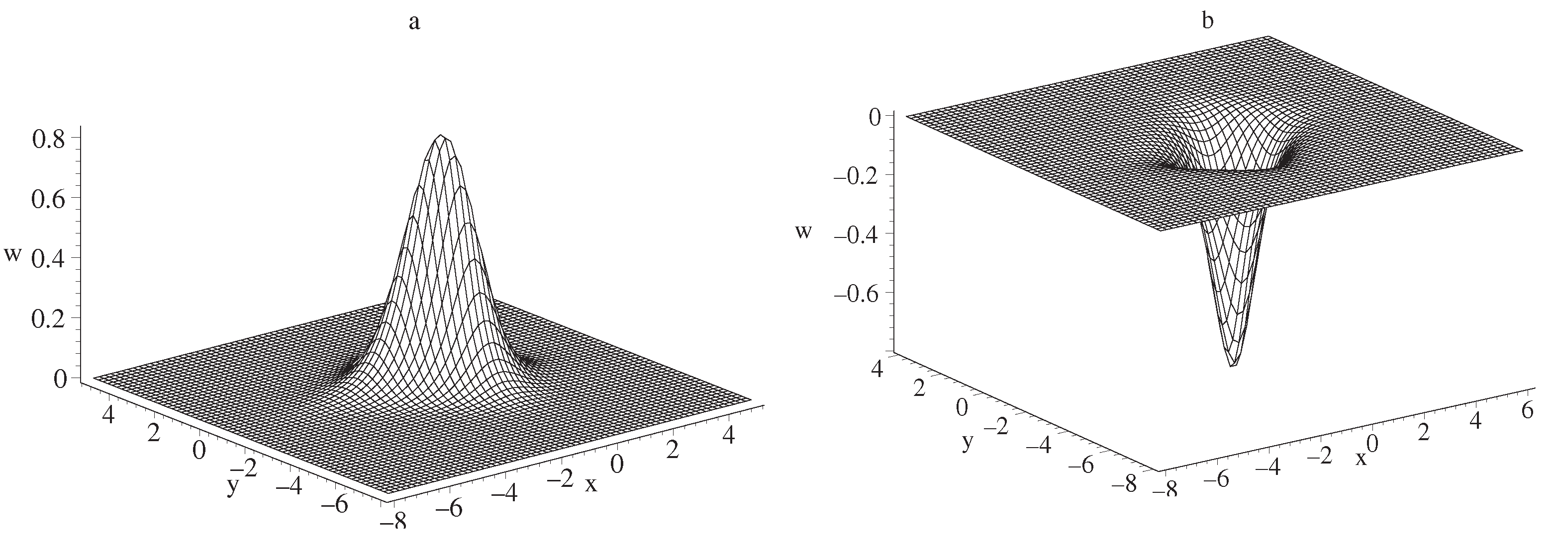
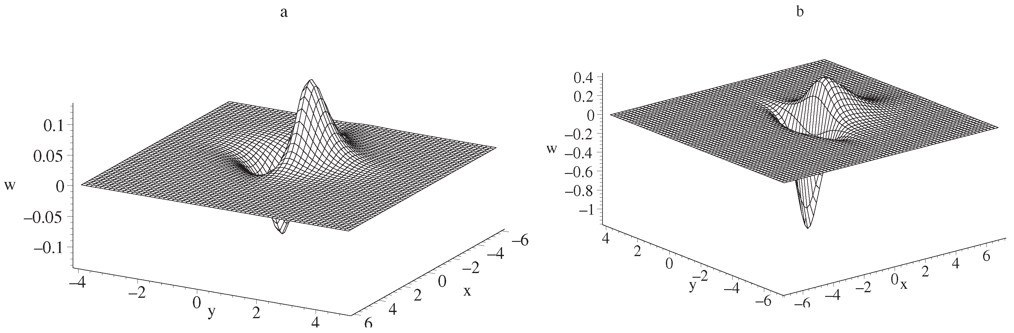
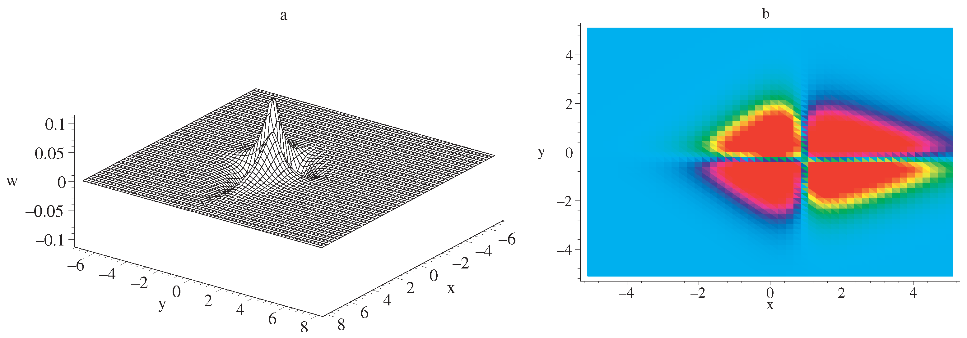
3.1. Special Localized Solutions of SWW Equation

In order to obtain resonant dromion, lump and solitoff solutions, we impose restrictions on the functions p and q as

$$\begin{array}{c}\hfill p=\sum _{i=1}^{N}exp(k_{i}x+{\omega }_{i}t+x_{0i}),q=\sum _{h=1}^{J}exp(K_i+H_{i}y)\sum _{j=1}^{L}exp\left(M_{j}t\right),\end{array}$$

(14)

where $k_i,{\omega }_i,x_{0i},K_i,H_i$ and $M_j$ are the arbitrary constants, and $N,J$ and L are arbitrary and positive no-negative integers. Resonant dromion solution, lump and multiple solitoff solutions are given by selecting different parameters. Here, we select $N=J=L=2$ and $t=0$ to explain these phenomena.

A single resonant dromion solution is given by the parameters as

$$\begin{array}{c}{k}_1=1,{\omega }_1=2,x_{01}=1,k_2=2,{\omega }_2=\frac{1}{2},x_{02}=3,\\ K_1=1,H_1=2,M_1=3,K_2=2,H_2=2,M_2=\frac{1}{2}.\end{array}$$

(15)

The type of the bright and dark dromion is shown with $a_0=15,a_1=1,a_2=4,a_3=2$, $(a_0{a}_3-a_1{a}_2>0)$ and $a_0=3,a_1=1,a_2=40,a_3=2$, $(a_0{a}_3-a_1{a}_2<0)$ in Figure 1a,b, respectively.

Above the single resonant dromion solution, the same sign of the coefficients of the spaces $x,y$, i.e., ($k_1{k}_2>0$ and $H_1{H}_2>0$), is given. The dromion solution will transform the lump wave with the opposite sign, i.e., ($k_1{k}_2<0$ and $H_1{H}_2<0$). Two types of the lump waves are plotted in Figure 2, with parameters such as $a_0=15,a_1=1,a_2=4,a_3=2,k_1=1,{\omega }_1=2,x_{01}=1,k_2=2,{\omega }_2=\frac{1}{2},x_{02}=3,K_1=1,H_1=2,M_1=3,K_2=2,H_2=-2,M_2=\frac{1}{2}$. And, other parameters for $k_2$ and $M_1$ are $k_2=2,M_1=3$ and $k_2=-4,M_1=-3$ in Figure 2a,b, respectively. The amplitudes of the peak and valley are the symmetry and asymmetry in Figure 2a,b, respectively.

Another type of single dromion solution is given with $a_0=35,a_1=1,a_2=4,a_3=2,k_1=1,{\omega }_1=2,x_{01}=1,k_2=-2,{\omega }_2=\frac{1}{2},x_{02}=3,K_1=1,H_1=-2,M_1=-3,K_2=2,H_2=2,M_2=\frac{1}{2}$ in Figure 3.

The solitoff solutions are presented under the selections as $a_0=3,a_1=1,a_2=3,a_3=0,k_1=-1,{\omega }_1=1,x_{01}=1,k_2=-\frac{1}{3},{\omega }_2=\frac{1}{2},x_{02}=3,K_1=1,H_1=2,M_1=1,K_2=-\frac{1}{3},H_2=2,M_2=\frac{1}{2}$. Different types of solitoff solutions are obtained by different values of the coefficients of the spaces $x,y$. Other parameters for $k_1,k_2$ and $H_1$ are $k_1=-1,k_2=-\frac{1}{3},H_1=2$; $k_1=-1,k_2=\frac{1}{3},H_1=2$; $k_1=-1,k_2=-\frac{1}{3},H_1=-2$ and $k_1=-1,k_2=-\frac{1}{3},H_1=-2$ in Figure 4a–d, respectively.

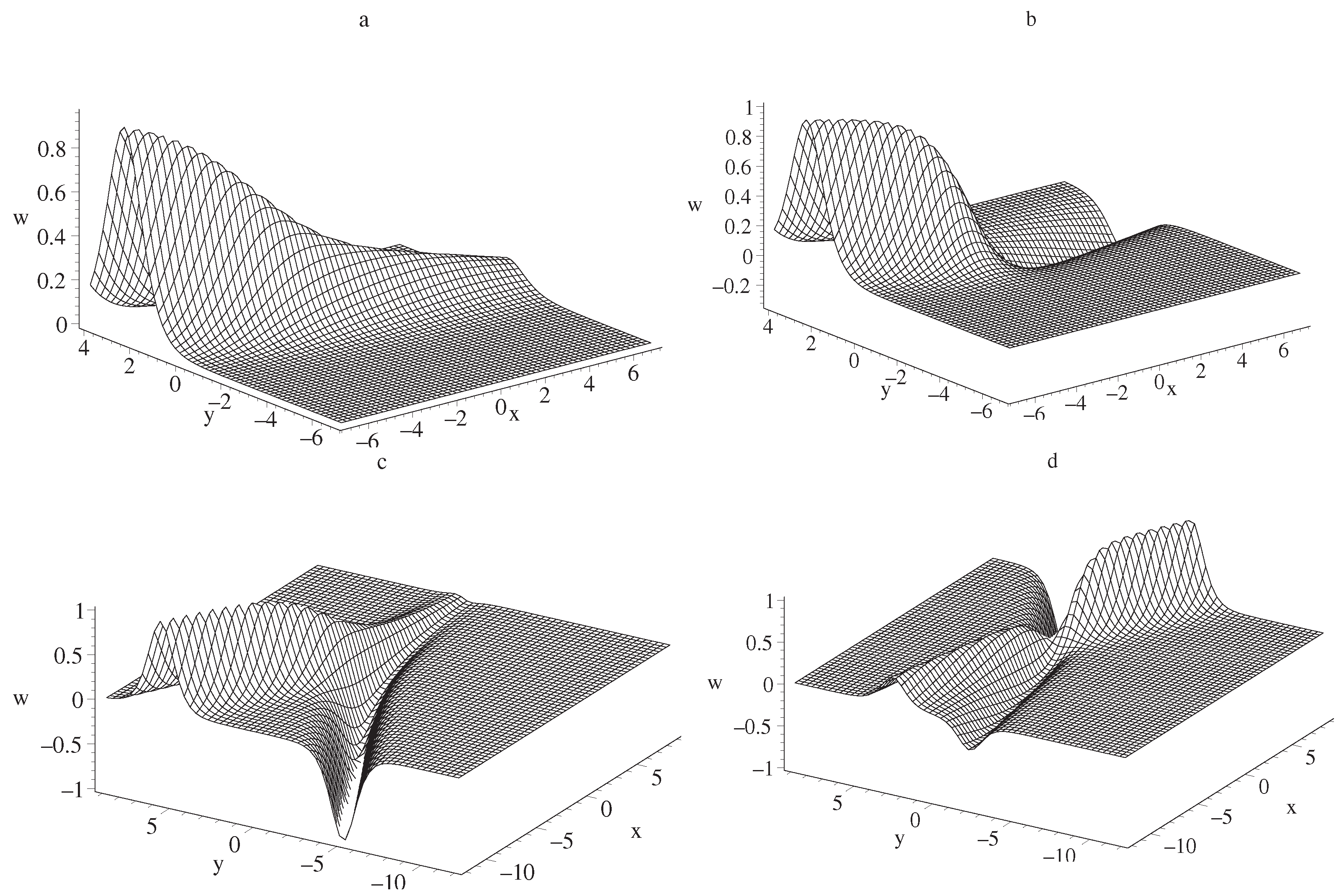
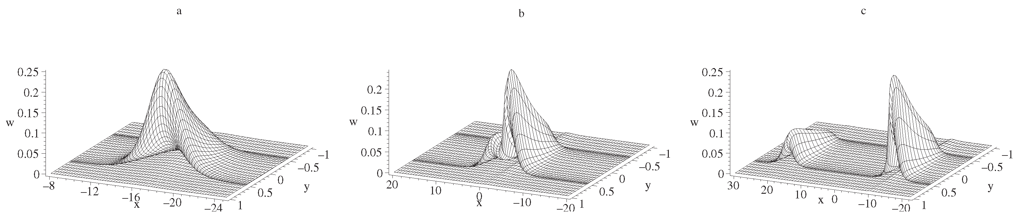
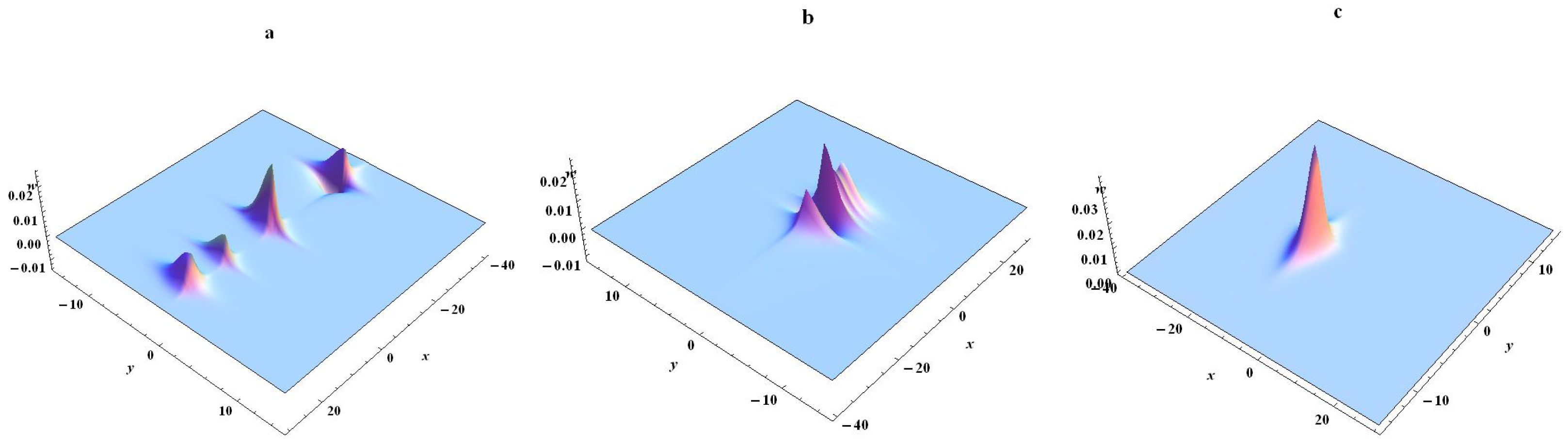
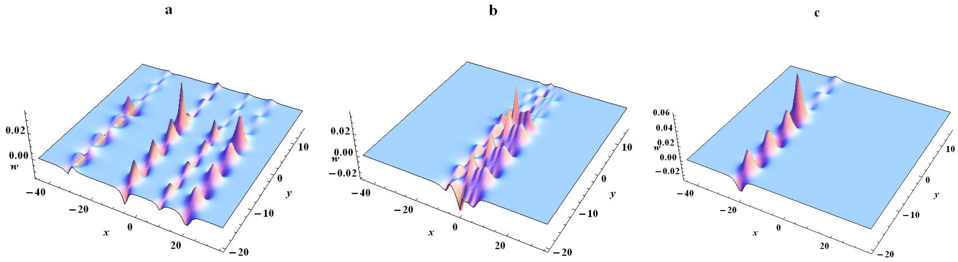
3.2. Special Fission and Fusion Phenomena of SWW Equation

In this part, we list certain specific forms of stable localized excitations for the quantity of w expressed by (13) for a suitable selecting of the arbitrary functions. Several innovative fission and fusion phenomena, such as the semifoldons, peakons, lump, dromions and periodic waves, are constructed both in analytical and graphical ways.

Semifoldon fission. In order to obtain a variety of the fission solitary wave solution for the formulation w, we restrict the functions p and q as

$$\begin{array}{c}p=1+2exp(x-2t)+\{\begin{array}{c}exp(x+t),x+t\le 0,\hfill \\ 2-exp(-x-t),x+t>0,\hfill \end{array}\\ q_y=A{\sec \mathrm{h}}^2\left(\zeta \right),y=\zeta -2tanh\left(\zeta \right),q={\int }^{\zeta }{q}_y{y}_{\zeta }d\zeta ,\end{array}$$

(16)

where A is an arbitrary constant. A variety of the fission solitary wave solution can be achieved by choosing p and q as (16). One provides the bell-like semifoldon fission and the anti-bell-like semifoldon by using $A<0$ and $A>0$, respectively. Here, we select $A=-1,(A<0)$ to explain the phenomena of the bell-like semifoldon fission in Figure 5. From Figure 5a–c, it shows that a bell-like semifoldon split into two bell-like semifoldons with time evolution. The bell-like semifoldons run in opposite directions along with the x-axis. The bell-like semifoldon with the smaller amplitude propagates in the forward direction of the x-axis, while the other one moves along the negative direction.

Semifoldon fusion. By choosing the arbitrary functions of p and q as

$$\begin{array}{cc}\hfill & p=2+2exp(2x+2t)+\frac{exp(2x-2t)}{1+exp(2x-2t)},\\ & q_y=B{\sec \mathrm{h}}^2\left(\zeta \right),y=\zeta -1.5tanh\left(\zeta \right),q={\int }^{\zeta }{q}_y{y}_{\zeta }d\zeta ,\end{array}$$

(17)

with the arbitrary constant B, a kind of semifoldon fusion solitary wave solution can be obtained by selecting p and q as (17). The bell-like semifoldon and the anti-bell-like semifoldon fusions are given with $B<0$ and $B>0$, respectively. One selects B = 1, ($B>0$) to explain the phenomena of the anti-bell-like semifoldon fusion in Figure 6. From Figure 6a–c, two anti-bell-like semifoldons fuse to the single anti-bell-like semifoldon with a time evolution.

Peakons’ and dromions’ fusion. By using the indeterminate functions of p and q as

$$\begin{array}{c}p=exp(1+x+2t)+exp(3+2x+\frac{t}{2})+1+\{\begin{array}{c}-ln\{tanh\left[\frac{1}{3}(1-x+t)\right]\},x\le t,\hfill \\ ln\{tanh\left[\frac{1}{3}(1+x-t)\right]\}-2ln[tanh\left(\frac{1}{3}\right)],x>t,\hfill \end{array}\\ +\{\begin{array}{c}-ln\{tanh\left[\frac{1}{3}(1-x-2t)\right]\},x\le -2t,\hfill \\ Pln\{tanh\left[\frac{1}{3}(1+x+2t)\right]\}-2ln[tanh\left(\frac{1}{3}\right)],x>-2t,\hfill \end{array},\\ q=[exp(1+2y)+exp(2+2y)][exp\left(3t\right)+exp\left(\frac{t}{2}\right)]+\{\begin{array}{c}-ln\{tanh\left[\frac{1}{3}(1-y)\right]\},y\le 0,\hfill \\ ln\{tanh\left[\frac{1}{3}(1+y)\right]\}-2ln[tanh\left(\frac{1}{3}\right)],y>0,\hfill \end{array}\end{array}$$

(18)

the interaction between two peakons and two dromions can be obtained with parameters as $a_0=15,a_1=1,a_2=4,a_3=2$ in Figure 7. Two peakons and two dromions are in a time evolution. These two peakons and two dromions will fuse to one dromion around $t=-2$.

Peakons, lump and dromions’ fusion. The lump wave is the rational function solution which can be localized in all directions of spaces. There has been a growing interest in investigating the lump wave [29,30]. Interactions among peakons, lump and dromions have a crucial role in the study of the nonlinear wave. By using the unconstrained functions of p and q as

$$\begin{array}{cc}\hfill & p=exp(1+x+4t)+\frac{2}{3+{(x-6t)}^2}+1+\{\begin{array}{cc}-ln\{tanh\left[\frac{1}{2}(1-x+t)\right]\},\hfill & x\le t,\hfill \\ ln\{tanh\left[\frac{1}{2}(1+x-t)\right]\}-2ln[tanh\left(\frac{1}{2}\right)],\hfill & x>t,\hfill \end{array}\\ & +\{\begin{array}{cc}-ln\{tanh\left[\frac{1}{2}(1-x-2t)\right]\},\hfill & x\le -2t,\hfill \\ ln\{tanh\left[\frac{1}{2}(1+x+2t)\right]\}-2ln[tanh\left(\frac{1}{2}\right)],\hfill & x>-2t,\hfill \end{array},\\ & q=\{\begin{array}{cc}-ln\{tanh\left[\frac{1}{2}(1-y)\right]\},\hfill & y\le 0,\hfill \\ ln\{tanh\left[\frac{1}{2}(1+y)\right]\}-2ln[tanh\left(\frac{1}{2}\right)],\hfill & y>0,\hfill \end{array}\end{array}$$

(19)

the interaction among two peakons, one lump and one dromion can be obtained with parameters such as $a_0=1,a_1=1,a_2=1,a_3=2$ in Figure 8. With a time evolution, two peakons, one lump and one dromion will fuse to one dromion around $t=-1$.

Peakons, lump, dromions and periodic waves fusion. By adding a periodic function $\frac{1}{cos(y-5t)+3}$ based on the form (19) of q, the interaction among two peakons, one lump, one dromion and periodic waves is shown with parameters as $a_0=2,a_1=1,a_2=1,a_3=2$ in Figure 9. One novel fusion phenomenon is derived with a time evolution. These solutions fuse to one dromion and the periodic wave around $t=-2$.

4. Conclusions

In summary, the MLVSA is successfully applied to the (2+1)-dimensional SWW equation. The solution with two arbitrary variable-separated functions is constructed. Taking into account the specified quantity, (13), and selecting suitable functions as p and q, the resonant dromion solution, lump, multiple solitoff solutions, semifoldons’ fission, semifoldons, peakons, lump, dromions and periodic waves’ fusion phenomena are investigated. Based on the parameters in (15), the type of the bright and dark dromion can be derived by selecting different parameters $a_0,a_1,a_2$ and $a_3$. By using other parameters, the dromion solution will translate into a lump wave. The amplitudes of the peak and valley for lump waves are symmetric and asymmetrical in Figure 2. Four types of solitoff solutions are constructed by selecting different parameters. Soliton phenomena with a fission and fusion have been observed in many real physical models, such as optic fibers [31] and photonic fibers [32]. The experimental results for the type of semifoldons’ fission, and semifoldons, peakons, lump, dromions and periodic waves’ fusion phenomena, are a significant area of research. We analyzed these phenomena both in analytical and graphical ways. One bell-like semifoldon splits into two bell-like semifoldons by means of (16). By selecting the arbitrary functions p and q as the form (17), two anti-bell-like semifoldons integrate to the single anti-bell-like semifoldon with a time evolution. Two peakons and two dromions, as well as two peakons, one lump and one dromion can be blended as one dromion by using different functions. Two peakons, one lump, one dromion and periodic waves become similar to dromion and periodic waves by introducing a periodic wave in the arbitrary function of q. Moreover, some other types of localized excitations, such as instantons, ring solitons, chaotic and fractal patterns are analyzed by selecting the corresponding arbitrary functions. By combining the velocity resonance mechanism, dromion molecules of the (3+1)-dimensional nonlinear systems are discussed [33,34]. Folded solitary waves and the corresponding superimposed structures of an extended (3+1)-dimensional KP-Boussinesq equation are systematically studied by exploring suitable multi-valued functions [35]. In our future work, these properties of the (2+1)-dimensional SWW equation will study the combination of the velocity of the resonance mechanism.

References

1. Ablowitz, M.J.; Clarkson, P.A. Soliton, Nonlinear Evolution Equations and Inverse Scattering; Cambridge University Press: Cambridge, UK, 1999. [Google Scholar]
2. Jin, X.W.; Lin, J. Rogue wave, interaction solutions to the KMM system. J. Magn. Magn. Mater. 2020, 502, 166590. [Google Scholar] [CrossRef]
3. Jin, X.W.; Shen, S.J.; Yang, Z.Y.; Lin, J. Magnetic lump motion in saturated ferromagnetic films. Phys. Rev. E 2022, 105, 014205. [Google Scholar] [CrossRef] [PubMed]
4. Zhang, Z.; Yang, X.Y.; Li, B. Soliton molecules and novel smooth positons for the complex modified KdV equation. Appl. Math. Lett. 2020, 103, 106168. [Google Scholar] [CrossRef]
5. Zhu, J.Y.; Chen, Y. Data-driven solutions and parameter discovery of the nonlocal mKdV equation via deep learning method. Nonlinear Dyn. 2023, 111, 8397–8417. [Google Scholar] [CrossRef]
6. Fang, Y.; Wu, G.Z.; Wang, Y.Y.; Dai, C.Q. Data-driven femtosecond optical soliton excitations and parameters discovery of the high-order NLSE using the PINN. Nonlinear Dyn. 2021, 603–616, 105. [Google Scholar] [CrossRef]
7. Ren, B.; Cheng, X.P.; Lin, J. The (2+1)-dimensional Konopelchenko-Dubrovsky equation: Nonlocal symmetries and interaction solutions. Nonlinear Dyn. 2016, 86, 1855–1862. [Google Scholar] [CrossRef]
8. Yang, J.J.; Tian, S.F.; Li, Z.Q. Riemann-Hilbert problem for the focusing nonlinear Schrödinger equation with multiple high-order poles under nonzero boundary conditions. Physica D 2022, 432, 133162. [Google Scholar] [CrossRef]
9. Li, Y.; Tian, S.F.; Yang, J.J. Riemann-Hilbert problem and interactions of solitons in the n-component nonlinear Schrödinger equations. Stud. Appl. Math. 2022, 148, 577–605. [Google Scholar] [CrossRef]
10. Ma, W.X.; Seoud, E.Y.A.E.; Ali, M.R.; Sadat, R. Dynamical behavior and wave speed perturbations in the (2+1) pKP equation. Qual. Theor. Dyn. Syst. 2023, 22, 2–16. [Google Scholar] [CrossRef]
11. Hirota, R. The Direct Method in Soliton Theory; Cambridge University Press: Cambridge, UK, 2004. [Google Scholar]
12. Lou, S.Y.; Lu, J.Z. Special solutions from variable separation approach: Davey-Stewartson equation. J. Phys. A Math. Gen. 1996, 29, 4029–4215. [Google Scholar] [CrossRef]
13. Tang, X.Y.; Lou, S.Y.; Zhang, Y. Localized excitations in (2+1)-dimensional systems. Phys. Rev. E 2002, 66, 046601. [Google Scholar] [CrossRef]
14. Shen, S.F. (1+1)-dimensional coupled integrable dispersion-less system. Commun. Theor. Phys. 2005, 44, 779–782. [Google Scholar] [CrossRef]
15. Zhang, R.; Shen, S.F. A new exact solution and corresponding localized excitations of the (2+1)-dimensional mKdV equation. Phys. Lett. A 2007, 370, 471–476. [Google Scholar] [CrossRef]
16. Zheng, C.L.; Fang, J.P.; Chen, L.Q. New variable separation excitations of a (2+1)-dimensional Broer-Kaup-Kupershmidt system obtained by an extended mapping approach. Z. Naturforsch. A 2004, 59, 912–918. [Google Scholar] [CrossRef]
17. Dai, C.Q.; Zhou, G.Q. Exotic interactions between solitons of the (2+1)-dimensional asymmetric Nizhnik-Novikov-Veselov system. Chin. Phys. 2007, 16, 1201–1208. [Google Scholar]
18. Dai, C.Q.; Zhou, G.Q.; Zhang, J.F. Exotic localized structures based on variable separation solution of (2+1)-dimensional KdV equation via the extended tanh-function method. Chaos Soliton Fract. 2007, 33, 1458–1467. [Google Scholar] [CrossRef]
19. Dai, C.Q.; Zhang, J.F. Variable separation solutions for the (2+1)-dimensional generalized Nizhnik-Novikov-Veselov equation. Chaos Soliton Fract. 2007, 33, 564–571. [Google Scholar] [CrossRef]
20. Dai, C.Q.; Wang, Y.Y. Localized coherent structures based on variable separation solution of the (2+1)-dimensional Boiti-Leon-Pempinelli equation. Nonlinear Dyn. 2012, 70, 189–196. [Google Scholar] [CrossRef]
21. Dai, C.Q.; Chen, R.P. Solitons with fusion and fission properties in the (2+1)-dimensional modified dispersive water wave system. Z. Naturforsch. 2006, 61, 307–315. [Google Scholar] [CrossRef]
22. Dai, C.Q.; Zhang, J.F. New types of interactions based on variable separation solutions via the general projective Riccati equation method. Rev. Math. Phys. 2007, 19, 195–226. [Google Scholar] [CrossRef]
23. Dai, C.Q. Semifoldons with fusion and fission properties of (2+1)-dimensional nonlinear system. Chaos Soliton Fract. 2008, 38, 474–480. [Google Scholar] [CrossRef]
24. Quan, J.F.; Tang, X.Y. New variable separation solutions and localized waves for (2+1)-dimensional nonlinear systems by a full variable separation approach. Phys. Scr. 2023, 98, 125269. [Google Scholar] [CrossRef]
25. Dong, H.H.; Zhang, Y.F. Exact periodic wave solution of extended (2+1)-dimensional shallow water wave equation with generalized D p ¯ -operators. Commun. Theor. Phys. 2015, 63, 401–405. [Google Scholar] [CrossRef]
26. Roshid, H.O.; Ma, W.X. Dynamics of mixed lump-solitary waves of an extended (2+1)-dimensional shallow water wave model. Phys. Lett. A 2018, 382, 3262–3268. [Google Scholar] [CrossRef]
27. He, L.C.; Zhang, J.W.; Zhao, Z.L. M-lump and interaction solutions of a (2+1)-dimensional extended shallow water wave equation. Eur. Phys. J. Plus 2021, 136, 192. [Google Scholar] [CrossRef]
28. Alsufi, N.A.; Fatima, N.; Noor, A.; Gorji, M.R.; Alam, M.M. Lumps and interactions, fission and fusion phenomena in multi solitons of extended shallow water wave equation of (2+1)-dimensions. Chaos Soliton Fract. 2023, 170, 113410. [Google Scholar] [CrossRef]
29. Ma, W.X.; Zhou, Y. Lump solutions to nonlinear partial differential equations via Hirota bilinear forms. J. Differ. Equ. 2018, 264, 2633–2659. [Google Scholar] [CrossRef]
30. Ma, W.X. Lump solutions to the Kadomtsev-Petviashvili equation. Phys. Lett. A 2015, 379, 1975–1978. [Google Scholar] [CrossRef]
31. Stegeman, G.I.; Segev, M. Optical spatial solitons and their interactions: Universality and diversity. Science 1999, 286, 1518–1523. [Google Scholar] [CrossRef]
32. Kartashov, Y.V.; Malomed, B.A.; Torner, L. Solitons in nonlinear lattices. Rev. Mod. Phys. 2011, 83, 247. [Google Scholar] [CrossRef]
33. Cui, C.J.; Tang, X.Y.; Cui, Y.J. New variable separation solutions and wave interactions for the (3+1)-dimensional Boiti-Leon-Manna-Pempinelli equation. Appl. Math. Lett. 2020, 102, 106109. [Google Scholar] [CrossRef]
34. Tang, X.Y.; Cui, C.J.; Liang, Z.F.; Ding, W. Novel soliton molecules and wave interactions for a (3+1)-dimensional nonlinear evolution equation. Nonlinear Dyn. 2021, 105, 2549–2557. [Google Scholar] [CrossRef]
35. Shao, C.; Yang, L.; Yan, Y.; Wu, J.; Zhu, M.; Li, L. Periodic, n-soliton and variable separation solutions for an extended (3+1)-dimensional KP-Boussinesq equation. Sci. Rep. 2023, 13, 15826. [Google Scholar] [CrossRef] [PubMed]
Figure 1. The type of the bright and dark dromion is plotted in (a,b), respectively.
Symmetry 16 00082 g001
Figure 2. Two types of the lump wave are plotted in (a,b), respectively.
Symmetry 16 00082 g002
Figure 3. Anothertype of single dromion solution is plotted in (a). The corresponding density plot is shown in (b).
Symmetry 16 00082 g003
Figure 4. A single solitoff solution, two solitoff solutions, three solitoff solutions and four solitoff solutions are shown in (ad), respectively.
Symmetry 16 00082 g004
Figure 5. The fission phenomena of the bell-like semifoldons are shown in Figure 1a–c with different times: (a) t = 8 ; (b) t = 1 ; (c) t = 10 .
Symmetry 16 00082 g005
Figure 6. The fusion phenomena of the anti-bell-like semifoldon are plotted in Figure 2a–c with different times: (a) t = 8 ; (b) t = 1 ; (c) t = 15 .
Symmetry 16 00082 g006
Figure 7. The fusion phenomena of two peakons and two dromions are plotted in Figure 3a–c with different times: (a) t = 12 ; (b) t = 2 ; (c) t = 1 .
Symmetry 16 00082 g007
Figure 8. The fusion phenomena of two peakons, one lump and one dromion are plotted in Figure 4a–c with different times: (a) t = 5 ; (b) t = 1 ; (c) t = 3 .
Symmetry 16 00082 g008
Figure 9. The fusion phenomena of two peakons, one lump, one dromion and periodic waves are plotted in Figure 5a–c with different times: (a) t = 5 ; (b) t = 1 ; (c) t = 5 .
Symmetry 16 00082 g009
Disclaimer/Publisher’s Note: The statements, opinions and data contained in all publications are solely those of the individual author(s) and contributor(s) and not of MDPI and/or the editor(s). MDPI and/or the editor(s) disclaim responsibility for any injury to people or property resulting from any ideas, methods, instructions or products referred to in the content.