Data-Driven Model Predictive Control for Uncalibrated Visual Servoing

Abstract

This paper addresses the image-based visual servoing (IBVS) control problem with an uncalibrated camera, unknown dynamics, and constraints. A novel data-driven uncalibrated IBVS (UIBVS) strategy is proposed, incorporated with the Koopman-based model predictive control (KMPC) algorithm and the adaptive robust Kalman filter (ARKF). First, to alleviate the need for calibration of the camera’s intrinsic and extrinsic parameters, the ARKF with an adaptive factor is utilized to estimate the image Jacobian matrix online, thereby eliminating the laborious camera calibration procedures and improving robustness against camera disturbances. Then, a data-driven MPC strategy is proposed, wherein the unknown nonlinear dynamic model is learned using the Koopman operator theory, resulting in a linear Koopman prediction model. Only input–output data are used to construct the prediction model, and hence, the proposed approach is robust against model uncertainties. Furthermore, with a symmetric quadratic cost function, the proposed approach solves the quadratic programming problem online, and visibility constraints as well as joint torque constraints are taken into account. As a result, the proposed KMPC scheme can be implemented in real time, and the UIBVS performance degradation which arises from the control torque constraints can be avoided. Simulations and comparisons for a 2-DOF robotic manipulator demonstrate the feasibility of the proposed approach. Simulation results further validate that the computation time of the proposed approach is comparable to the one of kinematic-based methods.

1. Introduction

Visual servoing control that utilizes visual feedback to guide the movements of the manipulator’s end-effector has been widely used in the field of robotics [1]. This approach enhances the manipulator’s versatility, expanding its applicability to unstructured environments.

Image-based visual servoing (IBVS) directly controls the manipulator using image feature errors. One class of IBVS approaches realizes visual tracking by directly using global image information for error regulation in the loop [2]. For example, Collewet et al. [3] use photometric information to achieve visual servoing tasks without image feature extraction; however, this method struggles with handling diffuse reflection targets. In addition, other types of global image information, such as histograms [4] or Gaussian mixtures [5], have been utilized.

Another important class of IBVS methods is the point featured-based method. Since the design of point feature-based IBVS methods is simple, they have been widely used in the field of robotic arm visual servoing tasks. Considering the complexity of the calibration process and the impact of camera distortion, uncalibrated image-based visual servoing (UIBVS) methods that do not require precise calibration of the camera’s intrinsic and extrinsic parameters have been studied in depth [6,7,8,9,10]. The transformation of feature points in vision space and the robotic workspace can be represented via the image Jacobian matrix, which is related to depth information, as well as the camera’s intrinsic and extrinsic parameters. Therefore, for the UIBVS problem, the control performance highly depends on the accuracy of the image Jacobian matrix estimation. However, the underlying transformation between the pose of the end-effector and the image coordinates of feature points is nonlinear. While the image Jacobian matrix is a linearized representation, it results in modeling uncertainties. Moreover, due to the presence of unknown process and measurement noise, accurately estimating the image Jacobian matrix remains a major challenge in the UIBVS problem.

Currently, most UIBVS methods [11,12,13,14] focus on the kinematic-based control, which involves tracking desired image feature points via controlling joint velocities. Despite their advantages in terms of simple controller design and high computation efficiency, these methods require the robotic manipulator to follow commanded speeds in real time, which is often impractical [15]. Furthermore, joint torque constraints are not considered, potentially leading to performance degradation issues.

Dynamic-based control methods have been well studied in robotic control, but they are not widely utilized in UIBVS. One problem resides in the fact that the dynamic model of the robot is nonlinear, which leads to the design of a nonlinear controller with high computation complexity, making real-time visual tracking difficult. In addition, uncertainties arise due to the inaccurate or unknown parameters of the robotic manipulator, such as joint inertia and mass. Designing the controller for systems with unknown dynamics also compromises control precisions. To tackle this problem, data-driven methods [16,17] which do not require the knowledge of the analytical models have been studied recently. However, practical constraints such as joint torque constraints and camera field of view constraints should be taken into account, posing additional challenges to dynamic-based UIBVS control methods.

Motivated by the above-mentioned discussions, in this paper, we propose a novel ARKF-KMPC algorithm for UIBVS control. The ARKF is used to estimate the image Jacobian matrix when both the camera’s intrinsic and extrinsic parameters are unknown, which eliminates the laborious camera calibration procedures and enhances the system’s robustness against camera disturbances. The Koopman operator is introduced to construct a linear dynamic model of the manipulator, and the MPC controller is used to solve the UIBVS problem with state and control constraints. The main contributions of this paper can be summarized as follows:

• To address the IBVS problem in presence of uncalibrated camera parameters, unknown dynamics, and state and control constraints, we propose an ARKF-KMPC approach in which the UIBVS controller is designed at the dynamic level. Compared to the kinematic-based IBVS methods [18,19], the proposed method is robust against model uncertainties, and performance degradation arising from control torque constraints could be avoided. In contrast to dynamic-based UIBVS methods, the proposed approach alleviates the need for the dynamic model and achieves real-time control performance.
• The proposed ARKF-KMPC approach could effectively handle the camera calibration issue. The ARKF is utilized to estimate the image Jacobian matrix online when both the camera’s intrinsic and extrinsic parameters are unknown, thereby eliminating the laborious camera calibration procedures and improving robustness against camera disturbances.
• It is the first time that the data-driven control strategy has been introduced for the UIBVS problem. The unknown nonlinear dynamic model is learned via Koopman operator theory, resulting in a linear Koopman prediction model. Consequently, with a symmetric quadratic cost function, the proposed approach allows for the utilization of quadratic programming (QP) for online optimization, significantly reducing the computation cost, and making the real-time dynamic-based UIBVS control feasible. Simulation results further validate that the computation time of the proposed approach is comparable to the one of kinematic-based methods.

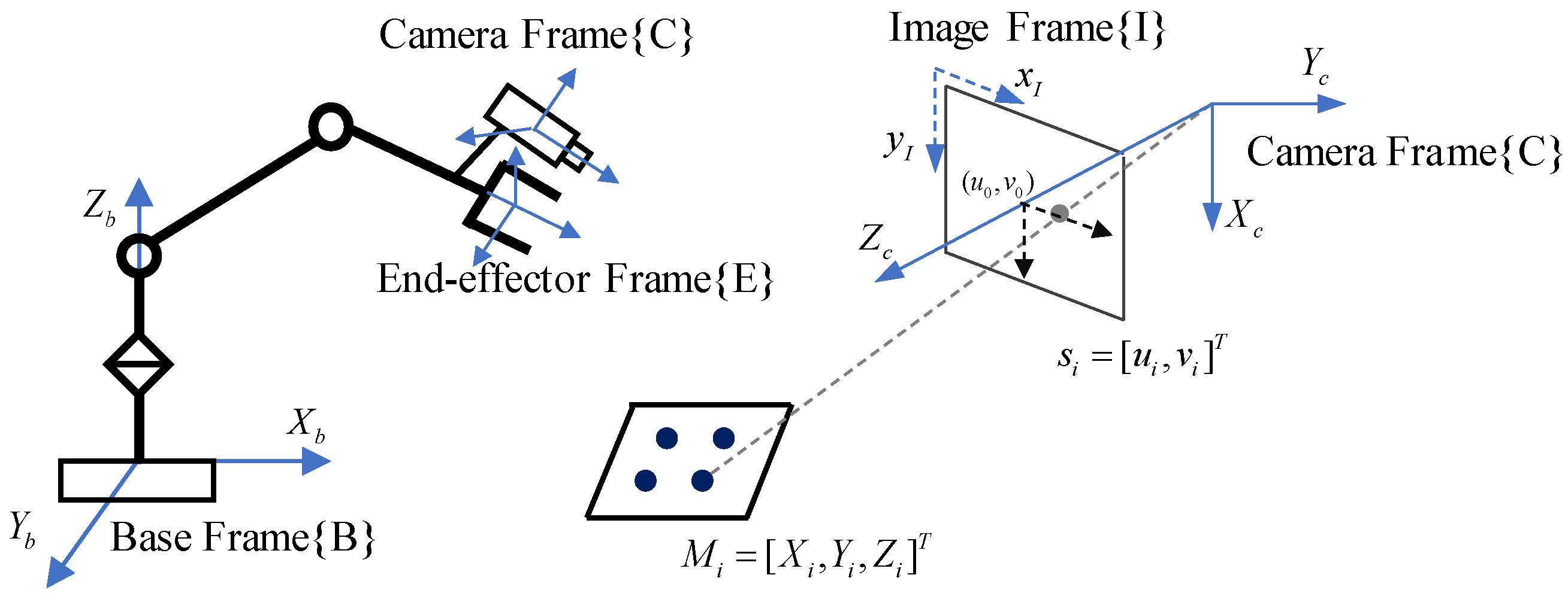
This paper is organized as follows. Section 2 introduces the related work of the paper. Section 3 introduces the mathematical model of the eye-in-hand camera configuration UIBVS system. Section 4 proposes the ARKF-KMPC algorithm for UIBVS. Simulations and comparisons are presented in Section 5, and conclusions are drawn in Section 6.

2. Related Work

UIBVS designs the control law based on the image Jacobian matrix; however, due to the nonlinearity of the robotics and uncertainties in camera parameters, deriving the image Jacobian matrix analytically is nontrivial. Recently, different methods have been proposed to enhance the accuracy and robustness of image Jacobian matrix estimation, such as Kalman filter [20], robust Kalman filter [21], extended Kalman filter [22], particle filter [23], and neural networks [24]. The Kalman filter method was first introduced into the estimation of the image Jacobian matrix by Qian et al. [20]. They constructed a dynamic system wherein the state variables of the system were composed of the elements of the image Jacobian matrix. Subsequently, a Kalman–Bucy filter was employed to online estimate the state variables of the system. The designed filter demonstrated robustness to system noise and external disturbances. Zhong et al. [21] proposed a UIBVS scheme based on the robust Kalman filter, in conjunction with Elman neural network (ENN) learning techniques. The relationship between the vision space and the robotic workspace was learned using an ENN, and then a robust KF was used to improve the ENN learning result. Wang et al. [25] proposed to estimate the total Jacobian matrix using the unscented particle filter, which can make full use of the feature measurements, and hence, can result in more accurate estimations. Gong et al. [23] proposed a geometric particle filter for visual tracking and grasping of moving targets. The introduction of these methods has facilitated research in UIBVS; however, due to the discrepancy between the actual nonlinear transformation and the linearized image Jacobian matrix, the process noise of the image Jacobian matrix estimation model is actually unknown, and hence, how to improve the estimation accuracy without sacrificing real-time performance remains an open problem.

Once the image Jacobian matrix is estimated, different control strategies have been proposed for addressing the UIBVS problem. For example, Chaumette et al. [11] designed the PD controller based on the pseudo-inverse of the image Jacobian matrix. Siradjuddin et al. [12] designed a distributed PD controller of a 7 degrees-of-freedom (DOF) robot manipulator for tracking a moving target. The reinforcement learning algorithm was proposed to adaptively tune the proportional gain in [14]. To address the problem of unknown dynamics, He et al. [26] proposed an eye-in-hand visual servoing control scheme based on the input mapping method, which directly utilizes the past input–output data for designing the feedback control law. The above-mentioned approaches could be used for online control; however, the state and control constraints in the UIBVS system are not taken into account.

Model Predictive Control (MPC) is also a method to solve the constraints in the control system [27,28,29], which involves the online solution of a finite-horizon open-loop optimization problem at each sampling instant. The first element of the obtained control sequence is then applied, and the process is repeated at the next sampling instant. MPC efficiently handles state and input constraints and could be implemented in real time. Consequently, MPC has been widely used in robotic control, and several MPC-based UIBVS methods have been developed. For example, Qiu et al. [18] proposed an adaptive MPC control scheme wherein the unknown camera intrinsic and extrinsic parameters, unknown depth parameters, as well as external disturbances are estimated via a modified disturbance observer. He et al. [19] proposed a synthetic robust MPC method with input mapping for the UIBVS problem under system constraints. However, these methods are designed only using the kinematics of robotics.

For the dynamic-based MPC methods of the UIBVS system, Qiu et al. [1] proposed an MPC controller based on the identification algorithm and the sliding mode observer. The unknown model parameters are estimated via the parameter identification algorithm, and the sliding mode observer is designed to estimate the joint velocities of the IBVS system. Wu et al. [30] introduced a two-layer MPC control scheme incorporating an extended state observer to address the problem of parameter uncertainties. Two MPC controllers were designed for both the kinematic level and the dynamic level sequentially, resulting in solving two optimal control problems online. As a result, designing the controller is complicated when tuning design parameters, and the performance of the dynamic controller highly depends on the performance of the kinematic controller. Moreover, both the above dynamic-based MPC methods are based on the nonlinear dynamic model of robotics, which results in solving the nonlinear optimization problem, and hence, is difficult to implement in real time.

Recently, data-driven MPC has been proposed to address the issue of unknown model parameters, wherein input–output data are used to learn the system model. For example, Gaussian Process (GP) [31] and neural networks [32] are employed for offline learning of prediction models, followed by online MPC controller design. However, online updates of GP models require tracking all measurement data, which may be computationally infeasible. Additionally, due to the nonlinearity of the neural network, the controller suffers from real-time implementation.

Koopman operator theory provides a data-driven solution by constructing a linear model of the nonlinear dynamical system, enabling the use of linear control methods like linear quadratic regulators (LQRs) and linear MPC [33]. For instance, Zhu et al. [34] proposed a Koopman MPC (KMPC) approach for trajectory tracking control of an omnidirectional mobile manipulator. Bruder et al. [35] designed MPC controllers for a pneumatic soft robot arm via the Koopman operator and demonstrated that the KMPC controllers outperform the MPC controller based on the linearized model, making accurate linear control of nonlinear systems achievable. However, to the best of the authors’ knowledge, few data-driven MPC strategies have been considered for solving the IBVS problems.

3. Preliminaries and Problem Formulation

In this section, the mathematical model of the eye-in-hand camera configuration UIBVS system is introduced, which includes the perspective projection model, image Jacobian matrix, manipulator dynamics model, and visual servoing control model.

3.1. Perspective Projection Control Model

The setup of the eye-in-hand camera configuration is shown in Figure 1. The feature point in the world (base) coordinate system is represented as $M_i={[X_i,Y_i,Z_i]}^T(i=1,\dots ,m)$. According to the perspective projection principle [36], the corresponding image feature points $s_i={[u_i,v_i]}^T$ on the image plane are given as

$$\left[\begin{array}{c}{u}_i\\ v_i\\ 1\end{array}\right]=\frac{1}{Z_i}\left[\begin{array}{cccc}{\alpha }_x& 0& u_0& 0\\ 0& {\alpha }_y& v_0& 0\\ 0& 0& 1& 0\end{array}\right]{\mathit{T}}_{\mathit{e}}^{\mathit{c}}{\mathit{T}}_{\mathit{b}}^{\mathit{e}}\left[\begin{array}{c}{X}_i\\ Y_i\\ Z_i\\ 1\end{array}\right],$$

(1)

where $\left[\begin{array}{cccc}{\alpha }_x& 0& u_0& 0\\ 0& {\alpha }_y& v_0& 0\\ 0& 0& 1& 0\end{array}\right]$ is the camera intrinsic matrix. The parameters ${\alpha }_x$ and ${\alpha }_y$ represent the focal lengths in two directions in pixels, respectively. ${[u_0,v_0]}^T$ represents the principal point of the image plane. ${\mathit{T}}_{\mathit{e}}^{\mathit{c}}$ denotes the homogeneous transformation matrix between the end-effector frame and the camera frame. ${\mathit{T}}_{\mathit{b}}^{\mathit{e}}$ denotes the homogeneous transformation matrix of the end-effector with respect to the base frame, which can be calculated via the forward kinematics of the robot manipulator.

3.2. Image Jacobian Matrix

Denote the velocity of the end-effector (camera) as $\dot{\mathit{r}}=({\upsilon }_x,{\upsilon }_y,{\upsilon }_z,{\omega }_x,{\omega }_y,{\omega }_z)$; then, the velocity of the image feature ${[{\dot{u}}_i,{\dot{v}}_i]}^T$ could be obtained via kinematics of rigid bodies and projection principles as [11]

$${\dot{s}}_i=\left[\begin{array}{c}\dot{u_i}\\ \dot{v_i}\end{array}\right]=\underset{{\mathit{L}}_i}{\underbrace{\left[\begin{array}{cccccc}-\frac{{\alpha }_x}{Z_i}& 0& \frac{{\overline{u}}_i}{Z_i}& \frac{{\overline{u}}_i{\overline{v}}_i}{{\alpha }_x}& -\frac{{\overline{u}}_i^2}{{\alpha }_x}-{\alpha }_x& {\overline{v}}_i\\ 0& -\frac{{\alpha }_y}{Z_i}& \frac{{\overline{v}}_i}{Z_i}& \frac{{\overline{v}}_i^2}{{\alpha }_y}+{\alpha }_y& -\frac{{\overline{u}}_i{\overline{v}}_i}{{\alpha }_y}& -{\overline{u}}_i\end{array}\right]}}\dot{\mathit{r}},$$

(2)

where ${\mathit{L}}_i$ is known as the image Jacobian matrix of $s_i$, and ${\overline{u}}_i=u_i-u_0$, ${\overline{v}}_i=v_i-v_0$. The derivation of the image Jacobian matrix is shown in Appendix A.

Denote $\mathit{s}={[s_1,\dots ,s_m]}^T$ as the collection of all image feature points; then,

$$\dot{\mathit{s}}=\mathit{L}·\dot{\mathit{r}},$$

(3)

where $\mathit{L}={[{\mathit{L}}_1^T,\dots ,{\mathit{L}}_m^T]}^T\in {\Re }^{2m\times 6}$ is the overall image Jacobian matrix.

3.3. Kinematics and Dynamics of Robotic Manipulator

The forward kinematics equation of the robotic manipulator is represented as

$$\dot{\mathit{r}}={\mathit{J}}_{\mathit{r}}\left(\mathit{q}\right)·\dot{\mathit{q}},$$

(4)

where $\mathit{q}\in {\Re }^n$ represents the joint angle vector of the manipulator, n is the degree of the robotic manipulator, and ${\mathit{J}}_{\mathit{r}}\left(\mathit{q}\right)$ represents the robotic Jacobian matrix.

The dynamic model of the robotic manipulator is given by [37]

$$\mathit{M}\left(\mathit{q}\right)\ddot{\mathit{q}}+\mathit{C}(\mathit{q},\dot{\mathit{q}})\dot{\mathit{q}}+\mathit{G}\left(\mathit{q}\right)=\mathit{\tau },$$

(5)

where $\mathit{M}\left(\mathit{q}\right)\in {\Re }^{n\times n}$ represents the symmetric inertia matrix, $\mathit{C}(\mathit{q},\dot{\mathit{q}})\in {\Re }^{n\times n}$ represents the centrifugal and Coriolis torque matrix, $\mathit{G}\left(\mathit{q}\right)\in {\Re }^{n\times 1}$ is the gravitational force vector, and $\mathit{\tau }\in {\Re }^{n\times 1}$ denotes the control input torque vector.

3.4. Image-Based Visual Servoing Control Model

Combining (3) and (4), the relationship between the motion of the feature in image space and the joint velocity in joint space is given as

$$\dot{\mathit{s}}=\mathit{L}·{\mathit{J}}_{\mathit{r}}\left(\mathit{q}\right)·\dot{\mathit{q}}.$$

(6)

Let ${\mathit{x}}_{\mathbf{1}}=\mathit{q}$, ${\mathit{x}}_{\mathbf{2}}=\dot{\mathit{q}}$; then, from (5) and (6), the overall discrete-time IBVS system model can be written as

$$\begin{array}{cc}\hfill \mathit{s}(k+1)& =\mathit{s}\left(k\right)+\mathit{L}\left(k\right){\mathit{J}}_{\mathit{r}}\left(k\right){\mathit{x}}_{\mathbf{2}}\left(k\right)\Delta t\hfill \end{array}$$

(7a)

$$\begin{array}{cc}\hfill {\mathit{x}}_{\mathbf{1}}(k+1)& ={\mathit{x}}_{\mathbf{1}}\left(k\right)+{\mathit{x}}_{\mathbf{2}}\left(k\right)\Delta t\hfill \end{array}$$

(7b)

$$\begin{array}{cc}\hfill {\mathit{x}}_{\mathbf{2}}(k+1)& ={\mathit{x}}_{\mathbf{2}}\left(k\right)+{\mathit{M}}^{-1}\left(\mathit{\tau }\left(k\right)-\mathit{C}{\mathit{x}}_{\mathbf{2}}\left(k\right)-\mathit{G}\right)\Delta t,\hfill \end{array}$$

(7c)

where $\mathit{s}\left(k\right)$, ${\mathit{x}}_{\mathbf{1}}\left(k\right)$, and ${\mathit{x}}_{\mathbf{2}}\left(k\right)$ represent the image feature points, joint angle, and joint angular velocity at time instant $k\Delta t$, respectively, and $\Delta t$ is the sampling time.

Therefore, in this paper, the control objective is to design the control input torque $\mathit{\tau }\left(k\right)$, such that, without knowing the exact camera intrinsic and extrinsic parameters, the manipulator could track the desired feature points ${\mathit{s}}_{\mathit{d}}$.

4. ARKF-KMPC Algorithm for UIBVS

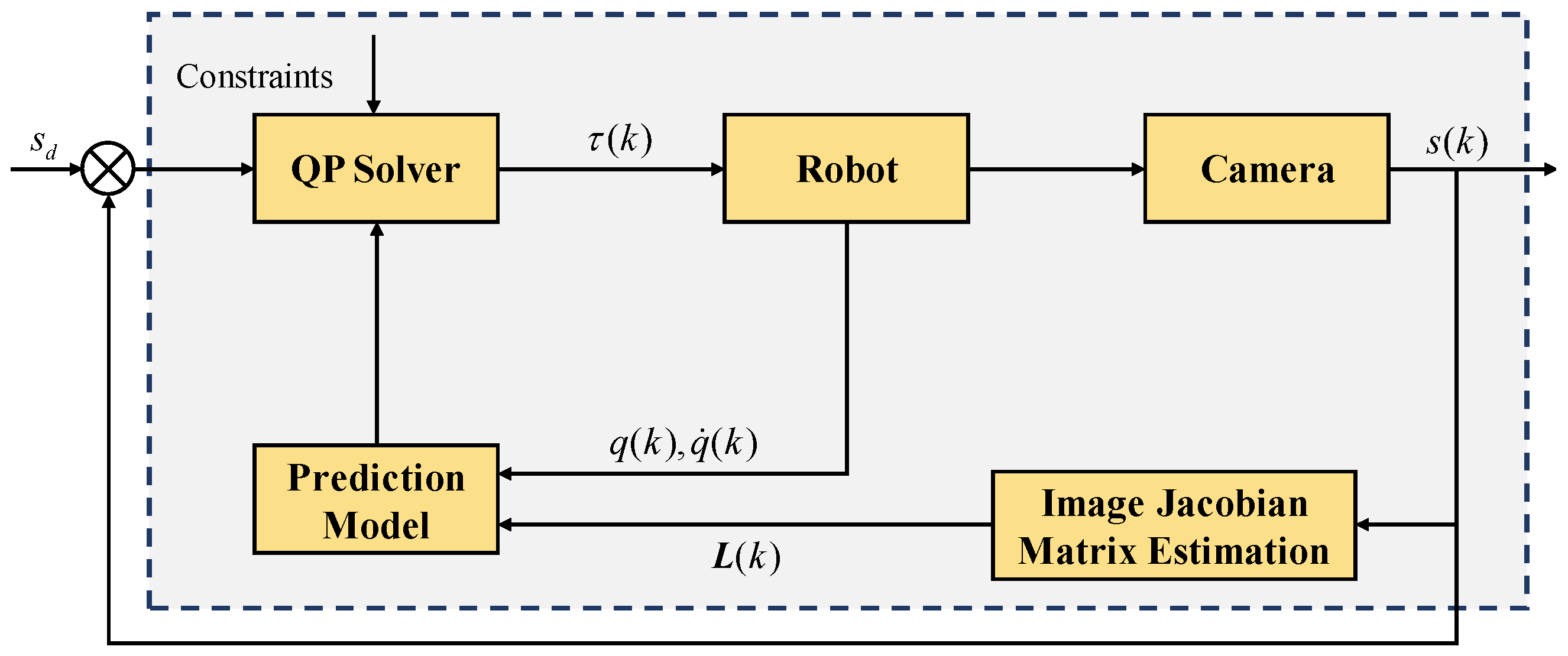
In this section, we propose a novel ARKF-KMPC algorithm for solving the UIBVS problem. The ARKF is introduced to estimate the image Jacobian matrix $\mathit{L}$; then, the Koopman operator is used to approximate the manipulator’s dynamic model, and the MPC controller is designed for the linear UIBVS model under state and control constraints. The uncalibrated visual servoing control system framework is shown in Figure 2.

4.1. Image Jacobian Matrix Estimation

Since the intrinsic and extrinsic parameters of the camera are unknown or varying, the ARKF algorithm [38] is proposed to estimate the image Jacobian matrix online. Denote $\mathsf{\Phi }\left(k\right)={[l_{1,1},\dots ,l_{2m,6}]}^T\in {\Re }^{(2m\times 6)\times 1}$ as an augmented state vector formed by collections of row elements of the image Jacobian matrix $\mathit{L}\left(k\right)$. The system observation vector is $Z\left(k\right)=\mathit{s}\left(k\right)-\mathit{s}(k-1)\in {\Re }^{2m}$, where $Z\left(k\right)$ represents the variation of image features. The image Jacobian matrix could be estimated via the discrete-time system [20]

$$\begin{array}{cc}\hfill \mathsf{\Phi }\left(k\right)& =\mathsf{\Phi }(k-1)+w\left(k\right)\hfill \end{array}$$

(8a)

$$\begin{array}{cc}\hfill Z\left(k\right)& =H\left(k\right)\mathsf{\Phi }\left(k\right)+\nu \left(k\right),\hfill \end{array}$$

(8b)

where $H\left(k\right)\in {\Re }^{2m\times (2m\times 6)}$ denotes the measurement matrix. $w\left(k\right)\in {\Re }^{(2m\times 6)\times 1}$ and $\nu \left(k\right)\in {\Re }^{2m}$ are the process noise and measurement noise, respectively.

The measurement matrix $H\left(k\right)$ could be written as

$$H\left(k\right)={\left[\begin{array}{ccc}\Delta r\left(k\right)\hfill & \hfill & \\ \hfill & \ddots \hfill & \\ \hfill & \hfill & \Delta r\left(k\right)\hfill \end{array}\right]}_{2m\times \left(2m\times 6\right)}.$$

(9)

where $\Delta r\left(k\right)$ represents the pose change of the camera (end-effector) between time k and $k-1$.

The state and covariance prediction equations are

$$\begin{array}{cc}\hfill \widehat{\mathsf{\Phi }}\left(k\right|k-1)& =\widehat{\mathsf{\Phi }}(k-1)\hfill \end{array}$$

(10a)

$$\begin{array}{cc}\hfill P\left(k\right|k-1)& =P(k-1)+Q\left(k\right),\hfill \end{array}$$

(10b)

where $\widehat{\mathsf{\Phi }}(k-1)$ and $P(k-1)$ represent the state estimation and error covariance matrix at time $k-1$, respectively. $Q\left(k\right)$ is the covariance matrix of the process noise.

Define the error of the state and measurement at time k as

$$\begin{array}{c}W\left(k\right)=\widehat{\mathsf{\Phi }}\left(k\right)-\widehat{\mathsf{\Phi }}(k\mid k-1)\\ V\left(k\right)=Z\left(k\right)-H\left(k\right)\widehat{\mathsf{\Phi }}\left(k\right)\end{array}.$$

(11)

Denote $R\left(k\right)$ as the covariance matrix of measurement noise, $P\left(k\right|k-1)$ as the error covariance matrix of predicted state vector $\widehat{\mathsf{\Phi }}\left(k\right|k-1)$, and $\alpha \left(k\right)$ is an adaptive factor with values $0<\alpha \left(k\right)\le 1$.

By using the least squares principle,

$$min(V^T\left(k\right)R^{-1}\left(k\right)V\left(k\right)+\alpha \left(k\right)W^T\left(k\right)P^{-1}\left(k\right|k-1)W\left(k\right)),$$

(12)

the estimator of the adaptive filter is

$$\widehat{\mathsf{\Phi }}\left(k\right)=\widehat{\mathsf{\Phi }}\left(k\right|k-1)+K\left(k\right)[Z\left(k\right)-H\left(k\right)\widehat{\mathsf{\Phi }}\left(k\right|k-1)],$$

(13)

where $K\left(k\right)$ is an adaptive gain matrix, and

$$K\left(k\right)=\frac{1}{\alpha \left(k\right)}P\left(k\right|k-1)H^T\left(k\right){\left[\frac{1}{\alpha \left(k\right)}H\left(k\right)P\left(k\right|k-1)H^T\left(k\right)+R\left(k\right)\right]}^{-1}.$$

(14)

The posterior error covariance matrix of the estimated state vector is

$$P\left(k\right)=\left[I-K\left(k\right)H\left(k\right)\right]P\left(k\right|k-1)/\alpha \left(k\right).$$

(15)

Furthermore, the adaptive factor $\alpha \left(k\right)$ is constructed based on the prediction residual, which is tuned automatically.

Define the prediction residual vector as

$$\epsilon \left(k\right)=Z\left(k\right)-H\left(k\right)\widehat{\mathsf{\Phi }}\left(k\right|k-1).$$

(16)

The theoretical calculated covariance matrix is

$$C_{\epsilon }\left(k\right)=H\left(k\right)P\left(k\right|k-1)H^T\left(k\right),$$

(17)

and the estimated covariance matrix is

$${\widehat{C}}_{\epsilon }\left(k\right)=\frac{1}{N}\sum _{i=1}^N\epsilon (k+1-i)\epsilon {(k+1-i)}^T,$$

(18)

where N is often chosen as 1 in practice. To verify whether the filter diverges, a statistical measure for discerning the adaptive factor is constructed by comparing the computed matrix $C_{\epsilon }\left(k\right)$ of $\epsilon \left(k\right)$ with the estimated matrix ${\widehat{C}}_{\epsilon }\left(k\right)$ as

$$\Delta \epsilon \left(k\right)={\left(\frac{tr\left({\widehat{C}}_{\epsilon }\left(k\right)\right)}{tr\left(C_{\epsilon }\left(k\right)\right)}\right)}^{1/2}.$$

(19)

An adaptive factor function model is constructed as

$$\alpha \left(k\right)=\left\{\begin{array}{cc}1& |\Delta \epsilon \left(k\right)|\le c_0\\ \frac{c_0}{|\Delta \epsilon (k\left)\right|}{\left(\frac{c_0-|\Delta \epsilon \left(k\right)|}{c_1-c_0}\right)}^2& c_0\le |\Delta \epsilon \left(k\right)|\le c_1\\ 0& |\Delta \epsilon \left(k\right)|>c_1\end{array}\right..$$

(20)

where $c_0$ and $c_1$ are design parameters, and usually, $c_0=1.0\sim 1.5$, $c_1=3.0\sim 8.0$.

The ARKF algorithm for the image Jacobian matrix estimation is summarized in Algorithm 1.

Algorithm 1 ARKF Algorithm.

Input: $\widehat{\mathsf{\Phi }}\left(0\right)$,$P\left(0\right)$,$Q\left(k\right)$,$R\left(k\right)$,$c_0$,$c_1$. Output: $\mathit{L}\left(k\right)$. for $k=1,2,\cdots$ do. Step 1. Predict state $\widehat{\mathsf{\Phi }}\left(k\right|k-1)$ and error covariance $P\left(k\right|k-1)$ via (10). Step 2. Calculate the adaptive factor $\alpha \left(k\right)$ via (16)–(20), where $Z\left(k\right)=S\left(k\right)-S(k-1)$ is the variation of image features, and $H\left(k\right)$ is defined in (9). Step 3. Update the posterior state $\widehat{\mathsf{\Phi }}\left(k\right)$ and error covariance $P\left(k\right)$ via (13)–(15). Step 4. Reorganize $\widehat{\mathsf{\Phi }}\left(k\right)$ for $\mathit{L}\left(k\right)$.

Remark 1.

Due to the nonlinearity of the visual servoing system of the robotic manipulator, applying the KF for estimating the image Jacobian matrix needs to satisfy the requirement that the manipulator should not move too fast; otherwise, the linear model (8a) is not valid. Furthermore, the model uncertainties $w\left(k\right)$ and $\nu \left(k\right)$ are not known a priori and may not be Gaussian white noise. From (12), it can be seen that the ARKF could adjust the weight of the prediction information, and hence, estimating the image Jacobian matrix via the ARKF could provide more accurate results [38].

4.2. Koopman Operator for Dynamical System

To tackle the problem where the system’s dynamic model is unknown, in this paper, we propose a data-driven modeling approach based on the Koopman theory. We briefly summarize procedures for constructing linear dynamical systems via Koopman operators. For further details, the reader may refer to the work [39,40].

Consider a discrete-time nonlinear dynamical system

$$x(k+1)=f\left(x\right(k\left)\right),$$

(21)

where $x\left(k\right)\in \mathcal{X}\subseteq {\mathcal{R}}^{n_x}$ is the system state, $\mathcal{X}$ is a non-empty compact set, and $f(·):\mathcal{X}\to \mathcal{X}$ is assumed to be a locally Lipschitz continuous nonlinear function.

Define a real-valued observable function of x as $g\left(x\right):\mathcal{X}\to \mathcal{R}$, and denote $\mathcal{G}$ as the space of observables. Koopman theory maps the nonlinear system (21) to a linear system using an infinite-dimensional linear operator $\mathcal{K}:\mathcal{G}\to \mathcal{G}$, which acts on the observable function, i.e.,

$$\mathcal{K}g\left(x\right(k\left)\right)=g\left(f\right(x\left(k\right)\left)\right)=g\left(x\right(k+1\left)\right).$$

(22)

Therefore, the Koopman operator $\mathcal{K}$ is a linear infinite-dimensional operator which propagates the observable $g\left(x\right(k\left)\right)$ to the next time step. In other words, the Koopman operator evolves nonlinear dynamics linearly without loss of accuracy.

Since the Koopman operator $\mathcal{K}$ is infinite-dimensional, a data-driven algorithm, extended dynamic mode decomposition (EDMD), is used to approximate $\mathcal{K}$ with a finite-dimensional operator ${\mathcal{K}}_d$ using collected data. A set of observables is used to lift the system from the original state space to a high-dimensional space, and the procedures are summarized as follows.

First, we select $N_{lift}$ observables $g_i,i=1,\dots ,N_{lift}$, and let

$$g\left(x\right)={[g_1\left(x\right),g_2\left(x\right),\cdots ,g_{N_{lift}}\left(x\right)]}^T.$$

(23)

We collect P snapshot pairs $\left[x\right(j),x(j+1\left)\right],j=1,\cdots ,P$, and construct the lifted data matrices

$$\begin{array}{cc}\hfill X_{1lift}& ={\left(\begin{array}{cccc}g\left(x\right(1\left)\right)& g\left(x\right(2\left)\right)& \cdots & g\left(x\right(P\left)\right)\end{array}\right)}_{N_{lift}\times P},\hfill \\ \hfill X_{2lift}& ={\left(\begin{array}{cccc}g\left(x\right(2\left)\right)& g\left(x\right(3\left)\right)& \cdots & g\left(x\right(P+1\left)\right)\end{array}\right)}_{N_{lift}\times P}.\hfill \end{array}$$

(24)

Then, the approximate Koopman operator ${\mathcal{K}}_d$ could be calculated by solving the least-squares problem

$$\underset{{\mathcal{K}}_d}{min}{\parallel X_{2lift}-{\mathcal{K}}_d{X}_{1lift}\parallel }_2^2.$$

(25)

where ${\parallel ·\parallel }_2$ represents the Euclidean vector norm [41].

Next, we generalize the Koopman theory to the controlled system:

$$x(k+1)=f\left(x\right(k),u(k\left)\right),$$

(26)

where $u\left(k\right)\in \mathcal{U}\subseteq {\mathcal{R}}^{n_u}$ is the control input at time step k. The extended state $\chi \left(k\right)={[x{\left(k\right)}^T,u{\left(k\right)}^T]}^T\in {\mathcal{R}}^{n_x+n_u}$ is defined, and the lifted data matrices are further extended as

$${\chi }_1=\left(\begin{array}{c}{X}_{1lift}\\ U\end{array}\right),{\chi }_2=\left(\begin{array}{c}{X}_{2lift}\\ U\end{array}\right),$$

(27)

where $U=\left[u\right(1),u(2),\cdots ,u(P\left)\right]$ such that $x(j+1)=f\left(x\right(j),u(j\left)\right),j=1,\cdots ,P$. Therefore, the finite-dimensional Koopman operator for the controlled system ${\mathcal{K}}_{du}$ can be obtained as the solution to the optimization problem

$$\underset{{\mathcal{K}}_{du}}{min}{\parallel {\chi }_1-{\mathcal{K}}_{du}{\chi }_2\parallel }_2^2.$$

(28)

Denote the linear Koopman model of (26) as

$$\begin{array}{cc}\hfill z_d(k+1)& =A_d{z}_d\left(k\right)+B_{d}u\left(k\right),\hfill \\ \hfill \widehat{x}\left(k\right)& =C_d{z}_d\left(k\right),\hfill \end{array}$$

(29)

where $z_d\left(k\right)=g\left(x\left(k\right)\right)\in {\mathcal{R}}^{N_{lift}}$ is the lifted state and $\widehat{x}\left(k\right)$ is the predicted value of the original state $x\left(k\right)$. Then, problem (28) is equivalent to

$$\underset{A_d,B_d}{min}{\parallel X_{2lift}-A_d{X}_{1lift}-B_{d}U\parallel }_2^2,$$

(30)

and the analytical solution is given as

$$[A_d,B_d]=X_{2lift}{[X_{1lift},U]}^{+},$$

(31)

where ${(·)}^{+}$ denotes the pseudoinverse of matrix $(·)$. $C_d$ is obtained by solving the least-squares problem

$$\underset{C_d}{min}{\parallel X-C_d{X}_{1lift}\parallel }_2^2,$$

(32)

where $X=\left[x\right(1),x(2),\dots ,x(P\left)\right]$, and the solution is given as

$$C_d=X{X}_{1lift}^{+}.$$

(33)

Furthermore, we choose observable functions

$$g\left(x\right)={[x^T,g_{n_x+1}\left(x\right),\cdots ,g_{N_{lift}}\left(x\right)]}^T,$$

(34)

i.e., the observable functions contain the original state; then,

$$C_d=[I_{n_x\times n_x},0].$$

(35)

The Koopman linear system identification algorithm is summarized in Algorithm 2.

Algorithm 2 Koopman Linear System Identification.

Input: $N_{lift}$. Output: $A_d$, $B_d$,$C_d$. Step 1. Collect P snapshot pairs $\left[x\right(j),x(j+1\left)\right]$ and $u\left(j\right)$ for $j=1,\cdots ,P$, where $x\left(j\right)={[x_1\left(j\right),x_2\left(j\right)]}^T$ and $u\left(j\right)=\tau \left(j\right)$. Step 2. Choose $N_{lift}$ observable functions $g_i,i=1,\cdots ,N_{lift}$ and construct the lifted data matrices via (25) and (28). Step 3. Identify the linear Koopman model (31) via (32) and (34).

Remark 2.

To train the Koopman model, we collect P input-state datasets ${[x\left(j\right),x(j+1),u\left(j\right)]}_{j=1}^P$, satisfying (26), and the data need not to be collected at consecutive time steps. The dimension of the lifted state space $N_{lift}$ is a design parameter, which should be selected according to the precision requirements. The observable functions $g_i$ can be chosen as some basis functions, such as Gaussian kernel functions, polyharmonic splines, and thin plate splines, or neural networks.

Remark 3.

A standard algorithm [39] is used to realize the Koopman model (29), and modifications of the algorithm are beyond the scope of this research. Recently, different algorithms have been proposed to improve the estimation accuracy of the model (29). For example, deep neural networks have been used to learn the observable functions [42], and instructions to construct a stable Koopman model have been studied in [43]. Stability analysis has been discussed in [43,44].

4.3. KMPC for UIBVS

Consider the nonlinear dynamic model of the manipulator (7b) and (7c), and let $\mathit{x}\left(k\right)={[{\mathit{x}}_{\mathbf{1}}^T\left(k\right),{\mathit{x}}_{\mathbf{2}}^T\left(k\right)]}^T\in {\Re }^{2n}$. We choose observable functions to contain the original state $\mathit{x}\left(k\right)$ as (34); then, the linear Koopman model (29) could be constructed, where $z_d\left(k\right)={[{\mathit{x}}_{\mathbf{1}}^T\left(k\right),{\mathit{x}}_{\mathbf{2}}^T\left(k\right),g_R^T\left(x\left(k\right)\right)]}^T$, and $g_R^T\left(x\left(k\right)\right)\in {\Re }^{N_{lift}-2n}$ represents the rest of the lifted states. Therefore, the overall linear UIBVS prediction model is

$$\begin{array}{cc}\hfill {\tilde{z}}_d(k+1)& ={\tilde{A}}_d{\tilde{z}}_d\left(k\right)+{\tilde{B}}_d\tau \left(k\right),\hfill \\ \hfill {\tilde{x}}_d\left(k\right)& ={\tilde{C}}_d{\tilde{z}}_d\left(k\right),\hfill \end{array}$$

(36)

where

$$\begin{array}{cc}\hfill {\tilde{A}}_d& =\left[\begin{array}{cccc}{I}_{2m\times 2m}& 0_{2m\times n}& {\mathit{LJ}}_{\mathit{r}}\Delta t& 0_{2m\times (N_{lift}-2n)}\\ 0_{N_{lift}\times 2m}& & A_{d_{N_{lift}\times N_{lift}}}\end{array}\right],\hfill \\ \hfill {\tilde{B}}_d& =\left[\begin{array}{c}0\\ B_d\end{array}\right],\hfill \\ \hfill {\tilde{C}}_d& =\left[\begin{array}{cc}{I}_{2m\times 2m}& 0\\ 0& C_{d_{2n\times N_{lift}}}\end{array}\right],\hfill \end{array}$$

(37)

and ${\tilde{z}}_d\left(k\right)=\left[\begin{array}{c}\mathit{s}\left(k\right)\\ z_d\left(k\right)\end{array}\right]$ is the extended state vector, ${\tilde{x}}_d\left(k\right)=\left[\begin{array}{c}\mathit{s}\left(k\right)\\ \widehat{x}\left(k\right)\end{array}\right]$ is the extended predicted value of states.

In the UIBVS, the image feature should remain within the image plane, so that the visibility constraints are defined as

$${\mathit{s}}_{\mathit{min}}\le \mathit{s}\left(k\right)\le {\mathit{s}}_{\mathit{max}},$$

(38)

where ${\mathit{s}}_{\mathit{min}}$ and ${\mathit{s}}_{\mathit{max}}$ are the image boundaries, respectively.

The control input constraints are defined as

$$\begin{array}{cc}\hfill {\mathit{\tau }}_{\mathit{min}}\le & \mathit{\tau }\left(\mathit{k}\right)\le {\mathit{\tau }}_{\mathit{max}}\hfill \end{array}$$

(39a)

$$\begin{array}{cc}\hfill \Delta {\mathit{\tau }}_{\mathit{min}}\le & \Delta \mathit{\tau }\left(\mathit{k}\right)\le \Delta {\mathit{\tau }}_{\mathit{max}},\hfill \end{array}$$

(39b)

where ${\mathit{\tau }}_{\mathit{min}}$ and ${\mathit{\tau }}_{\mathit{max}}$ are the minimum and maximum control input torques, respectively. $\Delta {\mathit{\tau }}_{\mathit{min}}$ and $\Delta {\mathit{\tau }}_{\mathit{max}}$ are the minimum and maximum control input increments, respectively.

Define the quadratic cost function at sampling time k as

$$\begin{array}{cc}\hfill J\left(k\right)& =\sum _{i=1}^{N_p-1}{∥{\mathit{s}}_{\mathit{d}}-\mathit{s}(k+i|k)∥}_{F^{*}}^2+{∥{\mathit{s}}_{\mathit{d}}-\mathit{s}(k+N_p|k)∥}_{R^{*}}^2\hfill \\ \hfill & +\sum _{i=1}^{N_p}{\parallel \mathit{\tau }(k+i-1|k)\parallel }_{G^{*}}^2,\hfill \end{array}$$

(40)

where $N_p$ is the prediction horizon, $F^{*}$, $G^{*}$, and $R^{*}$ are the weighting matrices. $\mathit{s}(k+i|k)$ denotes the predicted image feature points at time $k+i$ via prediction model (36) given the current state $\mathit{s}\left(k\right)$, $\mathit{\tau }(k+i-1|k)$ denotes the input at the time instant $k+i-1$.

The object of the UIBVS is to track the desired feature points ${\mathit{s}}_{\mathit{d}}$, and the optimization problem is formulated as follows:

$$\begin{array}{cc}\hfill \underset{{\left\{\mathit{\tau }(k+i-1|k)\right\}}_{i=1}^{N_p}}{min}& J\left(k\right),\hfill \\ \hfill \mathrm{s}.\mathrm{t}.& \left(36\right),\left(38\right),\left(39\right)\hfill \end{array}$$

(41)

At each sampling time, the optimal input sequence ${\left\{\mathit{\tau }(k+i-1|k)\right\}}_{i=1}^{N_p}$ is calculated by solving the open-loop finite-horizon optimal control problem. The first element of the sequence is considered as the optimal control input ${\mathit{\tau }}^{*}\left(k\right)$, and is applied to the robot. The process is repeated at the next sampling moment. Since $J\left(k\right)$ is a symmetric quadratic cost function, and the prediction model (36) is linear, the quadratic programming (QP) algorithm is used to solve the optimal control problem above.

Remark 4.

Compared to conventional visual servoing control methods [7,12,45], MPC is suitable for addressing situations with state and control constraints. Furthermore, in contrast to approaches in [18,30], the proposed method directly controls the joint torques of robotics, which can improve the control accuracy and robustness to external disturbances, enabling the control system to better adapt to complex working environments. Additionally, the symmetric cost function and the Koopman MPC strategy used in this paper result in a linear quadratic optimization problem, which could be solved via QP. This leads to a notable increase in computation speed, ensuring that real-time requirements are met and substantially enhancing the practical applicability of the proposed method.

The proposed ARKF-KMPC algorithm for UIBVS is summarized in Algorithm 3.

Algorithm 3 ARKF-KMPC Algorithm.

Input: Prediction horizon $N_p$, cost matrices $F^{*}$, $G^{*}$, $R^{*}$. Output: Control input ${\tau }^{*}$. Step 1. Koopman Linear System Identification. Identify the Koopman linear model $A_d$, $B_d$, $C_d$ via Algorithm 2. Step 2. for $k=0,1,2,\dots$ do. a. Image Jacobian Matrix Estimation. Estimate $\mathit{L}\left(k\right)$ via Algorithm 1, and update ${\tilde{A}}_d$ in (37). b. KMPC optimization. Solve (41) via QP to find the optimal input ${\tau }^{*}\left(k\right)$. c. Apply ${\tau }^{*}\left(k\right)$ to the UIBVS system.

5. Simulation Results

We test the proposed ARKF-KMPC method on a 2-DOF robotic manipulator. The parameters of the manipulator are shown in

Table 1. Parameters of the manipulator.

Notation	Parameters	Value	Unit
Length of link 1	$l_1$	0.45	m
Center length of link 1	$l_{c1}$	0.091	m
Center length of link 2	$l_{c2}$	0.048	m
Mass of link 1	$m_1$	23.902	kg
Mass of link 2	$m_2$	3.880	kg
Inertia of link 1	$H_1$	1.266	$\mathrm{kg}{\mathrm{m}}^2$
Inertia of link 2	$H_2$	0.093	$\mathrm{kg}{\mathrm{m}}^2$
Gravity acceleration	g	9.81	$\mathrm{m}/{\mathrm{s}}^2$

. The inertia matrix $\mathit{M}\left(\mathit{q}\right)$, the centripetal and Coriolis matrix $\mathit{C}(\mathit{q},\dot{\mathit{q}})$, and the gravitational torque vector $\mathit{G}\left(\mathit{q}\right)$ are defined in Appendix B [30].

Simulations are carried out with unknown dynamics, and the camera intrinsic parameters are unknown. The actual intrinsic parameters of the camera are set as follows: the focal length $f=0.008$ m, the coordinates of the principal points $(u_0,v_0)=(512,512)$ pixels. The image has a $1024\times 1024$ pixels resolution. The sampling time is 0.01s. The simulations are conducted in MATLAB with a 2.6 GHz Intel Core i5.

In general, root mean squared deviation (RMSD) is defined as

$$RMSD=\sqrt{\frac{1}{N_{sim}}\sum _{k=1}^{N_{sim}}{\parallel \Psi \left(k\right)-\overline{\Psi }\left(k\right)\parallel }_2^2},$$

(42)

where $\Psi \left(k\right)\in {\Re }^{n_0\times 1}$ is any $n_0$-dimensional actual state vector at time step k, and $\widehat{\Psi }\left(k\right)\in {\Re }^{n_0\times 1}$ represents the corresponding predicted state vector.

5.1. Verification of the Model Accuracy

First, we test the prediction accuracy of the Koopman model.

Training of the Koopman model. Data are collected over 1000 trajectories, with 100 snapshots in each trajectory. The control input for each trajectory is generated from a two-dimensional Gaussian distribution with zero mean and covariance of $2I_{2\times 2}$. The initial condition for each trajectory is randomly generated with a uniform distribution over $[-1,1]$. The observable functions are chosen to be the state itself, and the thin plate spline radial basis functions, where the center points are uniformly distributed in a given interval $[-1,1]$. The total number of observable states is $N_{lift}$.

In

Table 2. Comparisons of modeling errors.

	$\mathit{RMSD}$	${\mathit{T}}_{\mathit{max}}\left(\mathit{s}\right)$
${\mathit{N}}_{\mathit{lift}}$		0.15 s	0.5 s	2.0 s
65		0.1901	0.4390	1.6361
66		0.1884	0.3753	0.9543
69		0.1862	0.3754	2.5227
77		0.1927	0.5617	1.8364
80		0.1948	0.5410	2.5043
86		0.1862	0.3814	2.0103
102		0.1862	0.4226	1.9516

, we compare the prediction performance of different Koopman models during a short duration of $0.15$ s, a medium duration of $0.5$ s, and a long duration of 2 s. For each model, a Monte Carlo simulation with 1000 randomly generated initial conditions is conducted, and the RMSDs over the entire prediction horizon are shown in Table 2 as a function of $N_{lift}$.

It should be noted that prediction errors do not necessarily decrease as $N_{lift}$ increases, and the prediction performance for the short, medium, and long durations are different. For example, the best prediction performance can be achieved when $N_{lift}=69$ for the short duration but it performs the worst for the long duration. Therefore, the design parameter $N_{lift}$ should be tuned by trial-and-error.

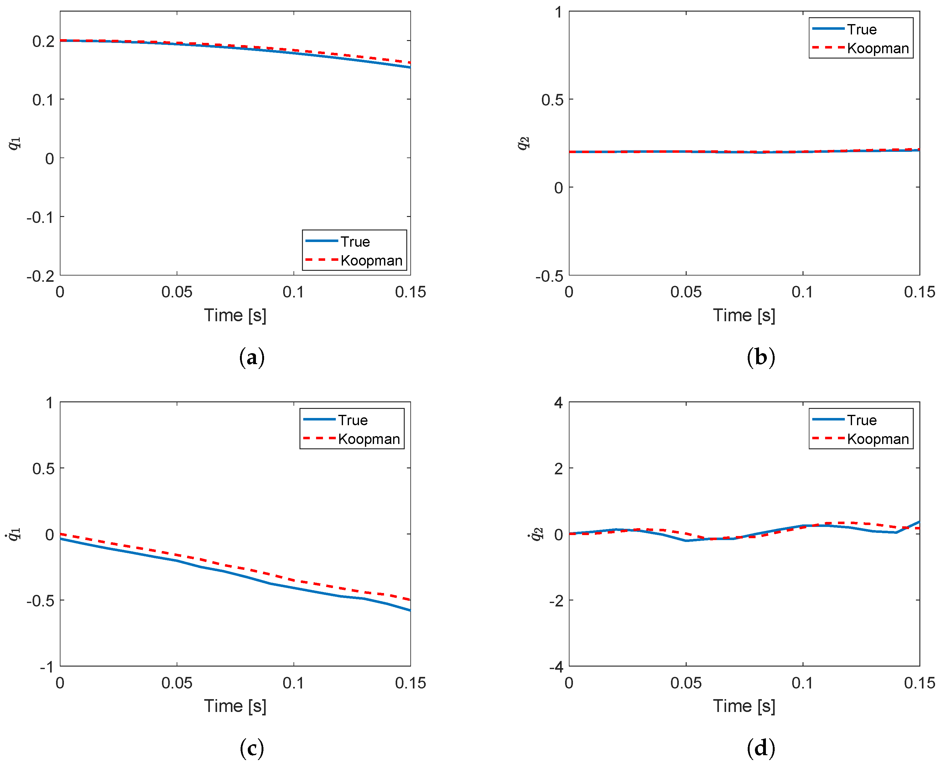
Testing of the Koopman model. In Figure 3, we compare the prediction results between the original nonlinear dynamic model (7b) and (7c), and the proposed Koopman model with $N_{lift}=66$ within a duration of 0.15s. It can be seen that predictions using the Koopman model are rather accurate.

5.2. Verification the Control Performance of the Model

Next, we test the control performance of the proposed ARKF-KMPC method. The visibility constraints are set as

$$\left[\begin{array}{c}0\\ 0\end{array}\right]pixels\le \mathit{s}\le \left[\begin{array}{c}1024\\ 1024\end{array}\right]pixels.$$

(43)

The control input constraints are set as

$$\begin{array}{cc}\hfill \left[\begin{array}{c}-0.5\\ -0.5\end{array}\right]Nm\le & \Delta \mathit{\tau }\le \left[\begin{array}{c}0.5\\ 0.5\end{array}\right]Nm\hfill \end{array}$$

(44a)

$$\begin{array}{cc}\hfill \left[\begin{array}{c}-10\\ -10\end{array}\right]Nm\le & \mathit{\tau }\le \left[\begin{array}{c}10\\ 10\end{array}\right]Nm.\hfill \end{array}$$

(44b)

The control objective is to map four feature points from their initial positions to desired positions on the image plane, with an error tolerance of four pixels, i.e.,

$${\parallel e\left(k\right)\parallel }_2={\parallel \mathit{s}\left(k\right)-{\mathit{s}}_{\mathit{d}}\parallel }_2\le 4.$$

(45)

The initial positions of the feature points on the image plane are ${(529.5,97.8)}^T$ pixels, ${(729.5,297.8)}^T$ pixels, ${(729.5,97.8)}^T$ pixels, and ${(529.5,297.8)}^T$ pixels, respectively. The desired positions of the feature points on the image plane are ${(454.8,377.7)}^T$ pixels, ${(654.8,577.7)}^T$ pixels, ${(654.8,377.7)}^T$ pixels, and ${(454.8,577.7)}^T$ pixels, respectively. For image Jacobian matrix estimation, the weighting matrices are chosen as $P=10I_{48\times 48}$, $Q=0.1I_{8\times 8}$, and $R=0.1I_{8\times 8}$, and the design parameters are $c_0=1.0$ and $c_1=3.0$. For the MPC controller, the weighting matrices are chosen as $F^{*}=I_{8\times 8}$, $G^{*}=100I_{8\times 8}$, and $R^{*}=0.1I_{2\times 2}$. To balance the computation time and control efficiency, the prediction horizon is chosen as $N_p=0.15$ s. The dimension of the Koopman model is chosen as $N_{lift}=66$.

Figure 4 shows simulation results for a 2-DOF robotic manipulator. The error curve ${\parallel e\left(k\right)\parallel }_2$ between the four actual feature points and the desired ones is shown in Figure 4a, where the smallest error is $3.7793$ pixels. In Figure 4b, the 2-D trajectory of the feature points on the image plane is presented. It can be seen that the robotic manipulator can reach the desired position successfully. The control input torques of the joints are shown in Figure 4c, from which we can observe that the joint torques and the increment of joint torques are always within the constraints. Joint angles of the 2-DOF manipulator are shown in Figure 4d, which changes smoothly. The average optimization time at each time step is $0.0009$ s, comfortably meeting real-time requirements.

Furthermore, we conducted 100 Monte Carlo simulations for models with different values of $N_{lift}$.

Table 3. Control errors for different models.

Model(${\mathit{N}}_{\mathit{l}\mathit{i}\mathit{f}\mathit{t}}$)	65	66	69	77	80	86	102
Error(pixels)	3.7723	3.7641	3.8262	3.2758	3.1437	3.8592	3.7712

presents the average final control errors for different models. The results further corroborate the effectiveness of the proposed control algorithm.

We also compare the proposed method with the method using the original nonlinear dynamics model. Although the image feature points using the nonlinear dynamic model converge to the desired ones with a smaller error of $2.72$ pixels, the average computation time is $5.4201$ s, which results from solving the nonlinear optimization problem using fmincon, and hence, is not suitable in real applications.

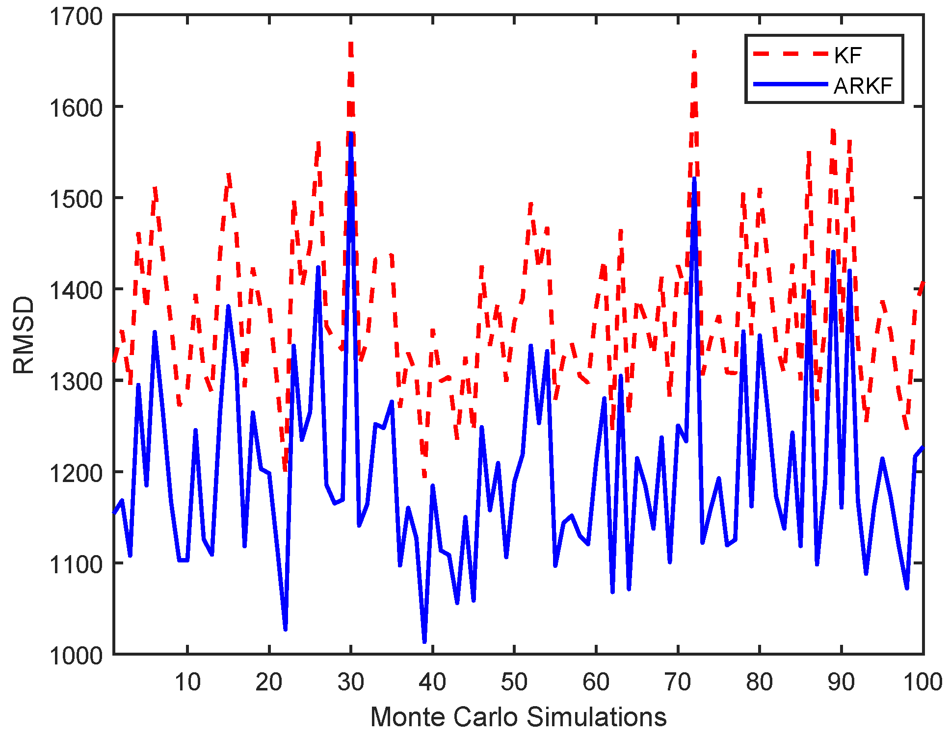
Furthermore, to validate the performance of the proposed ARKF algorithm for image Jacobian matrix estimation, we compare the RMSD between the estimated image Jacobian matrix and the actual image Jacobian matrix using KF and ARKF. We perform 100 Monte Carlo simulations; in each simulation, the control inputs are randomly generated from a two-dimensional Gaussian distribution with zero mean and a covariance of $2I_{2\times 2}$, over a simulation time of 6 s. The average RMSD of 100 Monte Carlo simulations using the KF algorithm is 1.3716 $\times {10}^3$ and 1.1995 $\times {10}^3$ using the ARKF. The RMSDs in 100 Monte Carlo simulations for both algorithms are presented in Figure 5.

It can be seen that, compared to the KF method, applying the ARKF for estimating the image Jacobian matrix effectively reduces the estimation error, enabling the system to perform visual servoing tasks accurately.

5.3. Comparisons with Related Work

To further demonstrate the superiority of the proposed algorithm, a comparative analysis is conducted against three related methods, as detailed in

Table 4. Comparison with existing methods.

Methods	Kinematics	Dynamics	Error (pixels)	Time (s)
(a)	MPC	×	7.3696	0.0005
(b)	MPC	PID	8.9505	0.0014
(c)	MPC	MPC	18.3579	1.5778
Ours	×	KMPC	3.7793	0.0009

. For all methods, the kinematic-based MPC is solved using QP, and design parameters are all tuned for best performance.

Method (a) designs the MPC controller only considering the kinematics of the manipulator, resulting in the fastest convergence rate. The average computation time for this method is about 0.0005 s per time step, which is the lowest among four algorithms; however, the final image error is 7.3696 pixels, which cannot satisfy the control performance requirement.

Both Methods (b) and (c) design two controllers for kinematics and dynamics separately. The joint angular velocities are optimized via the kinematic-based MPC controller, and the PD controller and MPC controller are designed at the dynamic level to track the desired joint angular velocities, respectively. It can be seen that, without sacrificing too much computation time, the position control using the PD controller is feasible, and the final image error of Method (b) is comparable to that of Method (a); however, the joint torque constraints are not considered when using the PD controller. On the other hand, Method (c) needs to solve a nonlinear optimization problem at each time step, and the average computation time is around 1.5778 s, which could not be implemented in real time. Moreover, the control performance of both Methods (b) and (c) highly depends on the results from the kinematic-based MPC controller, and the selection of design parameters also poses challenges in this problem.

Therefore, from Table 4, it can be seen that the proposed ARKF-KMPC method, which designs the dynamic-based MPC controller directly, could achieve the best performance. With a linear Koopman prediction model and a symmetric quadratic cost function, a linear optimization problem is solved at each time step, the computation time of the proposed approach is comparable to the one of the kinematic-based MPC controller and is significantly reduced when compared to Method (c). Moreover, the proposed approach is a data-driven control approach which does not need the actual dynamic model, making it robust to model uncertainties.

6. Conclusions

In this paper, we propose an ARKF-KMPC scheme for the data-driven control of constrained UIBVS systems. First, when the intrinsic and extrinsic parameters of the camera are unknown, the ARKF with an adaptive factor is utilized to estimate the image Jacobian matrix online. Then, the KMPC strategy is proposed to solve the UIBVS problem at the dynamic level. To address the issue of unknown dynamics, a linear Koopman prediction model is constructed via input–output data offline, resulting in a linear optimal control problem which is solved via QP online. The proposed UIBVS strategy is robust to imprecise camera calibration as well as unknown dynamics, with state and control constraints taken into account. Numerical simulations demonstrate that the proposed approach outperforms the kinematic-based control approaches, and the computation time of the proposed approach is comparable to the one of the kinematic-based control approach and has been significantly reduced when compared to the dynamic-based control approaches. The existing problem when estimating the image Jacobian matrix via the ARKF algorithm with a linear discrete-time system model is that the robotic manipulator should not move too fast. Therefore, the application of the proposed approach may be limited and the construction of a more realistic model for estimating the image Jacobian matrix could be further studied in future work. Also, the proposed approach is validated using the simulation, and future work will include testing the proposed method using data collected from actual experiments.