Density of States in the 3D System with Semimetallic Nodal-Loop and Insulating Gapped Phase

Abstract

We investigate a single-particle density of states in the three-dimensional system described by effective two-band Hamiltonian, which describes a ground state in two distant electronic phases: the semimetalic nodal-loop phase and the insulating gapped phase. An analysis of valence bands and Fermi surfaces in both phases indicates that the density of states crucially depends on the parameter in the Hamiltonian of the system that controls a topological alternation of the Fermi surface. The signature of that alternation is expected to play an important role in all quantities closely related to the density of electronic states, such as charge transport and the optical conductivity of the system for example.

1. Introduction

A number of physical properties of solids, expectantly those related to charge transport, are often described by so-called effective electron Hamiltonian, referring to the domain spanned over a small portion of the Brillouin zone in a restricted energy interval around the Fermi energy. Based on the underlying symmetry of the crystal lattice, at the specific points of the Brillouin zone, a minimal multi-band Hamiltonian can be constructed, which is sufficient to describe some single-particle and collective models of the system [1]. One such example is the Bernevig–Hughes–Zhang Hamiltonian [2], which appears to be sufficient to describe the electron properties of a number of systems mapped to it. In the case when two bands are located near the Fermi level and other bands are sufficiently far in energy, the minimal Hamiltonian can be further reduced to the two-band effective Hamiltonian represented by a $2\times 2$ matrix. The electron bands of the two-band effective Hamiltonian have an electron–hole symmetry and, in multiple cases, they are simple enough to permit an analytical result for a number of band-related calculations and obtained transport functions. Examples of systems whose electron bands are described by the two-band model are numerous and can be easily found in all three dimensions. We mention just some notable examples like the Su–Schrieffer–Heeger model (SSH) [3] and Peierls model [4] in 1D, massless and massive 2D Dirac system [5,6,7], Weyl systems or multiple Weyl point systems [8,9,10,11], massless 3D Dirac [12], Mexican-hat systems [13,14], nodal-line systems [15], and electron gas in a weak periodic potential [16].

In all of the mentioned systems, the single-particle and optical properties have been analytically derived, thus providing an insight into the underlying mechanisms and physical scales. In reality, however, many of specific properties that make the mentioned systems interesting are observed on small intrinsic energy scales no bigger then few meV around the Fermi energy. This also makes it challenging to experimentally distinguish between different possible ground states. For that reason, the single particle density of states (DOS) calculations is important since it provides direct information about electron bands. Those can be directly measured by, for example, measuring DOS at the Fermi energy via Pauli paramagnetic susceptibility or, indirectly, as a part of the joint density of states approach to the inter-band conductivity [17]. Generally, the number of analytically solvable electron models is rather small, which is exactly why every case of effective Hamiltonian yielding an analytical result is important. Besides an academic value, it provides a way to observe similarities in the electron properties between different models in various dimensions, by changing the parameters of the initial Hamiltonian promoted into the final result, precisely addressing the underlying mechanisms leading to them.

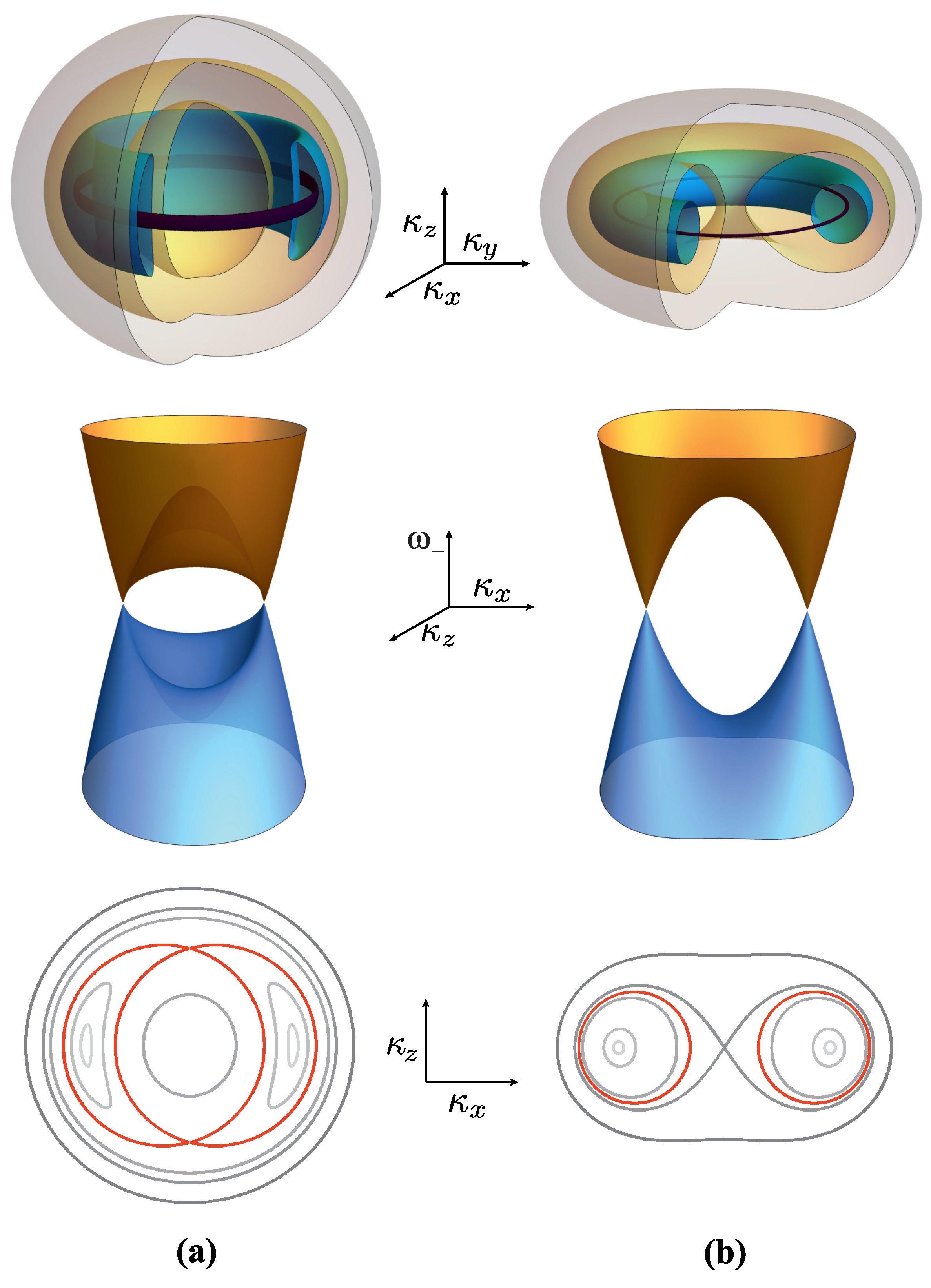
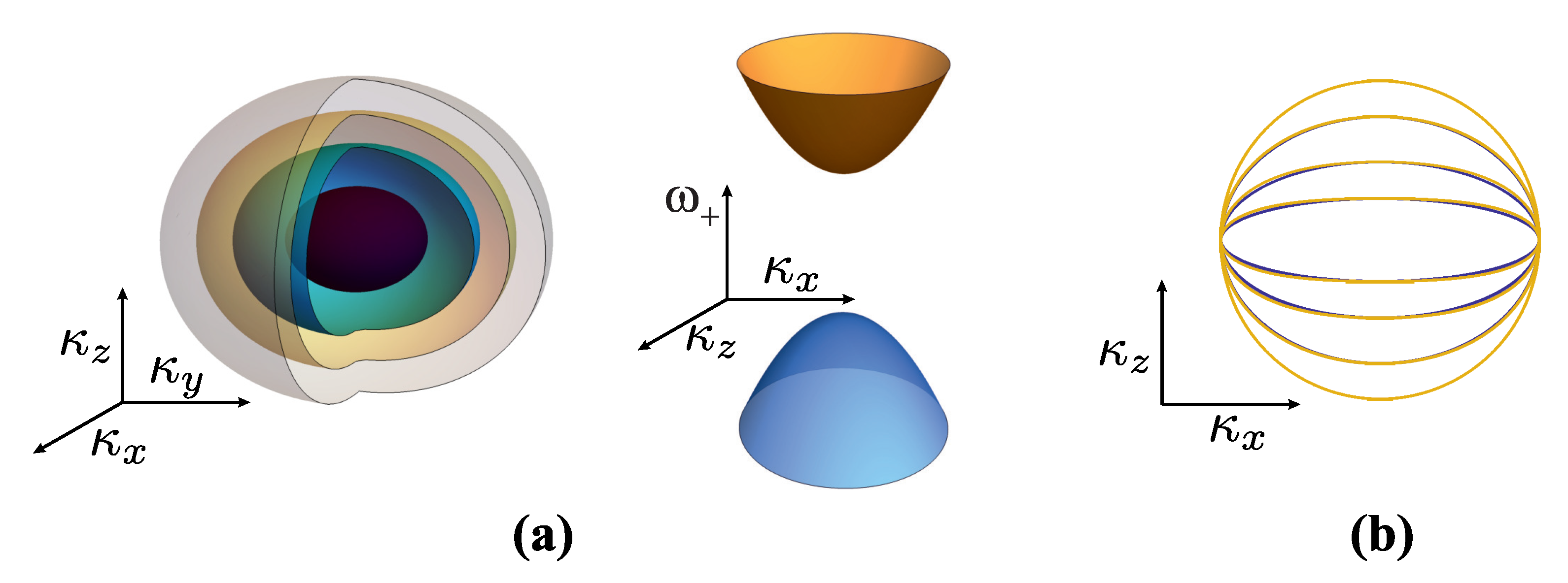
In this paper, we define and analyze the two-band effective Hamiltonian capable of describing two different electronic ground states (phases). The first one is the nodal-loop phase (NLP), and it is characterized by the touching of the valence bands over a ring. The second one is the gapped phase (GP), characterized by the separation of the valence bands by a finite energy gap. We find the corresponding electron dispersions for both phases and assume that the doping procedure (Fermi energy shifting) leaves the valence bands intact. We analyze the Fermi surface (FS) for each phase together with the identification of the van Hove points. Electron dispersions are presented in terms of dimensionless variables in which their properties are determined by a single parameter $\lambda$. It is shown that the NLP has a torus-like FS, which, depending on parameter $\lambda$, can be a doughnut-like or self-intersecting spindle, while the FS in the case of GP has a trivial shape related to usual doped 3D insulators. The DOS calculations are performed by finding the corresponding integration boundaries for each phase. Finally, the expressions for DOS in both phases are given. The DOS of both of the phases is analyzed in detail, with particular emphasis placed on the behavior near van Hove points and in connection to the parameter $\lambda$, where the DOS in the NLP showed a richer structure compared to the GP. It is our intention to use the two-band model in order to shed additional light upon otherwise complicated band structures that are inherent to the majority of the nodal-line systems [18,19].

2. The Two-Band Hamiltonian

The low-energy Hamiltonian of the 3D system under consideration, in the basis of the plane waves characterized by the wave vector $\mathbf{k}=(k_x,k_y,k_z)$, presented as a real $2\times 2$ matrix, reads

$$\widehat{H}=(\Delta +\nu b{k}^2){\sigma }_z+c{k}_z{\sigma }_x.$$

(1)

In the above expression, ${\sigma }_z$ and ${\sigma }_x$ are the Pauli matrices, while $\Delta$, b and c are positive parameters. Index $\nu =\pm 1$ is the phase index, with $\nu =-1$ denoting the NLP and $\nu =+1$ denoting the GP. Hamiltonian (1) contains the square of the total Bloch wave vector $k^2=k_x^2+k_y^2+k_z^2$. The diagonalization of Equation (1) is straightforward, yielding electron–hole symmetric eigenvalues for each phase $\nu$,

$${\epsilon }_{\nu }^{\pm }\left(\mathbf{k}\right)=\pm \sqrt{{(\Delta +\nu b{k}^2)}^2+c^2{k}_z^2}.$$

(2)

We scale electron dispersion Equation (2) to the gap parameter $\Delta$, introducing dimensionless variables ${\omega }_{\nu }^{\pm }\left(\mathit{\kappa }\right)={\epsilon }_{\nu }^{\pm }\left(\mathbf{k}\right)/\Delta$, $\mathit{\kappa }=\sqrt{b/\Delta }\mathbf{k}$ (i.e., ${\kappa }^2=k^{2}b/\Delta$) and parameter ${\lambda }^2=c^2/(b\Delta )$. We obtain the dispersions Equation (2) in dimensionless form

$${\omega }_{\nu }^{\pm }\left(\mathit{\kappa }\right)=\pm \sqrt{{(1+\nu {\kappa }^2)}^2+{\lambda }^2{\kappa }_z^2}$$

(3)

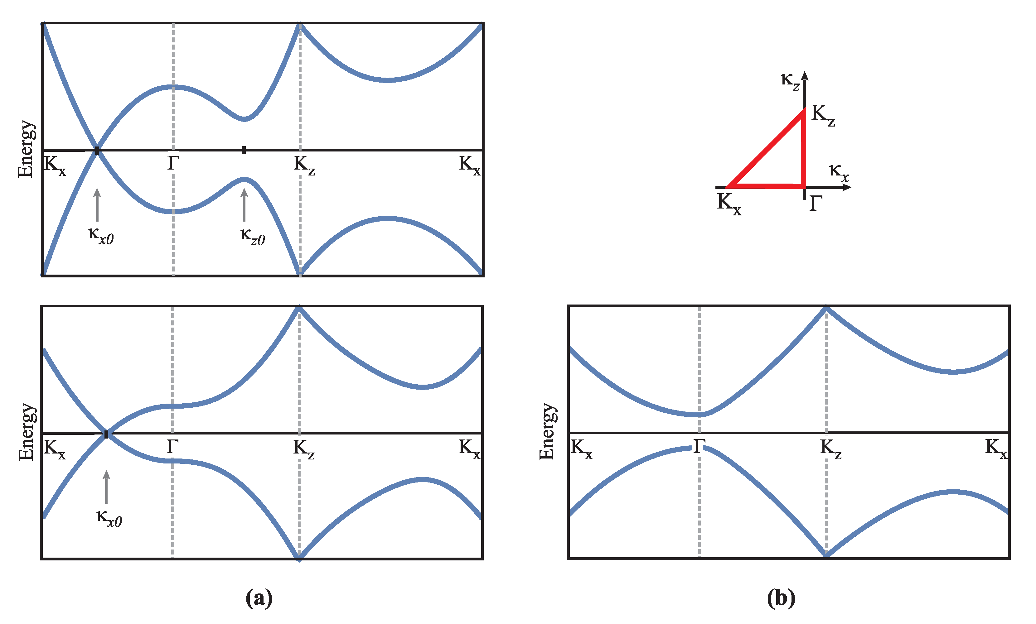
determined by two parameters: (1) the phase parameter $\nu =\pm 1$ essentially controlling the band topology, and (2) parameter $\lambda$ that controls the physical properties of bands, such as van Hove points and effective mass parameters. Below, we provide a detailed description of band properties.

3. Valence Bands and Fermi Surface

Here, we investigate the properties of electron dispersions Equation (3) and the Fermi surface in a doped system. Initially, we assume that both phases are undoped, i.e., that the Fermi level is located between the bands. The doping procedure consists of filling the conduction band ${\omega }_{\nu }^{+}\left(\mathit{\kappa }\right)$ up to some finite value of Fermi energy ${\omega }_F$ (in units of $\Delta$). An analytical analysis of the dispersion relation leads to the $\nu$-dependent polynomial in $\lambda$,

$$P_{\nu }\left(\lambda \right)=\frac{{\lambda }^4}{4}+\nu {\lambda }^2,$$

(4)

which appears to be important for further calculations and the description of the spectral properties as well as the DOS (it is shown in Figure 1). For $\nu =-1$ (NLP), $P_{-}\left(\lambda \right)$ is a non-monotonic function, i.e., $P_{-}\left(\lambda \right)\lessgtr 0$ for $\lambda \lessgtr 2$, with its minimum at $P_{-}(\lambda =\sqrt{2})=-1$, while for $\nu =+1$ (GP), $P_{+}\left(\lambda \right)$ is a positive monotonic function.

Figure 1. The $P_{\nu }\left(\lambda \right)$ polynomial according to Equation (4).

3.1. The Nodal-Loop Phase (NLP)

This phase appears for $\nu =-1$. In the intrinsic case, when the Fermi energy ${\omega }_F=0$, the main property of the NLP is the presence of the nodal ring of radius ${\kappa }_0=1$ located in the $({\kappa }_x,{\kappa }_y)$ plane along the touching line of two bands (3). If ${\omega }_F$ is increased, a doughnut-like Fermi surface emerges (see Figure 2). The exact properties of this Fermi surface depend on the value of parameter $\lambda$. There are two cases to be closely examined:

Figure 2. The NLP phase. The 3D Fermi surface (upper panel), the band energy, ${\omega }_{-}^{+}\left(\mathit{\kappa }\right)$ (brown) and ${\omega }_{-}^{-}\left(\mathit{\kappa }\right)$ (blue), dependence at ${\kappa }_y=0$ (middle panel), and its cross-section in the $({\kappa }_x,{\kappa }_z)$ plane (i.e., ${\kappa }_y=0$) (lower panel), determined by electron dispersion Equation (3). The FSs are shown at different dopings, i.e., the different value of the Fermi energy ${\omega }_F$, for (a) $\lambda =0.5\in (0,\sqrt{2})$ and (b) $\lambda =1.7\in (\sqrt{2},2)$. The Fermi energies ${\omega }_F$ in cross-sections are (in ascending shades of gray from light to dark): 0.1, 0.3, 0.8, 1, and 1.5. The red contour is for ${\omega }_F={\omega }_T\left(\lambda \right)$, i.e., 0.4841 in (a) and 0.8955 in (b).

(a)

Case $\lambda \in (0,\sqrt{2})$: The Fermi surface is shown in Figure 2a. As the Fermi energy ${\omega }_F$ increases from zero, the point-like (the nodal point) cross-section, along the ${\kappa }_x=0$, or ${\kappa }_y=0$, plane, evolves into two crescent shapes. As ${\omega }_F$ further increases, the crescent shapes are inflated and eventually touch each other, forming two self-intersecting circles. The FS at this particular Fermi energy ${\omega }_T$ is a type of torus called the self-intersecting spindle. The energy ${\omega }_T=\sqrt{-P_{-}\left(\lambda \right)}$ at which it occurs is the van Hove saddle point. The radius of each self-intersecting circle is $r=(\sqrt{1+{\omega }_T}+\sqrt{1-{\omega }_T})/2$, while their centers are displaced by $2R=\sqrt{1+{\omega }_T}-\sqrt{1-{\omega }_T}$ apart. For such a torus, it is evident that $R<r$. As ${\omega }_F$ increases further, the FS becomes composed of two ellipsoid-like surfaces (a smaller one centered inside the bigger one)—one decreasing and the other increasing in size—until ${\omega }_F=1$ is reached. At ${\omega }_F=1$, an elliptic van Hove point appears, at which the FS is a single ellipsoid-like surface. In the special case $\lambda =0$, the two bands touch over a sphere of radius ${\kappa }_0=1$. Then, if the Fermi energy is $0<{\omega }_F<1$, the FS comprises two concentric spheres and, if ${\omega }_F>1$, the FS is a single sphere.

(b)

Case $\lambda \in (\sqrt{2},2)$: The Fermi surface is shown in Figure 2b. As ${\omega }_F$ increases, the thickness of the “doughnut” reaches a special value when its cross-section with a plane ${\kappa }_x=0$, or ${\kappa }_y=0$, is two circles, i.e., the FS becomes a torus. As in the previous case, this happens at the particular value of Fermi energy, ${\omega }_T=\sqrt{-P_{-}\left(\lambda \right)}$. In this case, the FS forms a standard torus with radius of the circular cross-section $r=(\sqrt{1+{\omega }_T}-\sqrt{1-{\omega }_T})/2$ and a radius from the center of the torus to the center of the cross-section $R=(\sqrt{1+{\omega }_T}+\sqrt{1-{\omega }_T})/2>r$. As ${\omega }_F$ is increased with respect to ${\omega }_T$, two circles of the cross-section inflate, deform, and touch each other at ${\omega }_F=1$. This point is the van Hove saddle point, which is responsible for the kink in the DOS of the 3D system, as we shall show later. As ${\omega }_F$ is further increased, the FS attains an ellipsoidal-like shape.

(c)

Case $\lambda >2$: The Fermi surface shows no distinctive or interesting features other than a compact doughnut-like shape. We do not show it graphically.

3.2. The Gapped Phase (GP)

This phase appears for $\nu =+1$. Dominated by the band gap parameter $\Delta$, the FS of a doped gapped phase becomes a simple ellipsoid-like structure existing only for ${\omega }_F>1$ (see Figure 3a), in which parameter $\lambda$ increases the axial anisotropy, i.e., the larger $\lambda$ is, the flatter the ellipsoid (see Figure 3b) is. In fact, it can be shown that the FS can be, to an excellent approximation, written in terms of the reduced ellipsoid equation with the coefficients depending on the Fermi energy ${\omega }_F$ (measured from the middle of the band gap) and parameter $\lambda$,

$$\frac{{\kappa }_x^2}{{\omega }_F-1}+\frac{{\kappa }_y^2}{{\omega }_F-1}+\frac{{\kappa }_z^2}{\sqrt{{\omega }_F^2+P_{+}\left(\lambda \right)}-\sqrt{1+P_{+}\left(\lambda \right)}}=1.$$

(5)

Comparison of ${\kappa }_x=0$ or ${\kappa }_y=0$ plane cross section of (3) and (5) for various ${\omega }_F$ and $\lambda$ is shown in Figure 3b. In the special case $\lambda =0$, Equations (3) and (5) reduce to the equation for the sphere with the radius ${\kappa }_0=\sqrt{{\omega }_F-1}$.

Figure 3. The GP phase. (a) The 3D Fermi surface, for different values of ${\omega }_F>1$ (left panel), and the band energy, ${\omega }_{+}^{+}\left(\kappa \right)$ (brown) and ${\omega }_{+}^{-}\left(\kappa \right)$ (blue), dependence at ${\kappa }_y=0$ (right panel), determined by electron dispersion Equation (3). (b) The FS cross-section in the $({\kappa }_x,{\kappa }_z)$ plane at the Fermi energy ${\omega }_F=3.5$ for different $\lambda =0,2,4,8$ (rounder to flatter ellipses). The yellow curve is the exact result from Equation (3), while the blue curve is an approximation Equation (5).

Electron bands (3) in both NLP and GP phases are shown in Figure 4.

Figure 4. Electron bands (3) in (a) NLP ($\nu =-1$) and (b) GP ($\nu =+1$) phase along the characteristic directions in the momentum space (see the inset). The $\Gamma =(0,0)$ point is in the origin of momentum space, while ${\mathrm{K}}_{\mathrm{x},\mathrm{z}}$ are some points equally far away from the origin. Since the energy dependence on ${\kappa }_x$ and ${\kappa }_y$ are equivalent, all energies are plotted as ${\omega }_{\nu }^{\pm }({\kappa }_x,{\kappa }_y=0,{\kappa }_z)$. Bands ${\omega }^{+}$ (upper) and ${\omega }^{-}$ (lower) posses the electron–hole symmetry. For the NLP case (a), the parameter values are $\lambda =0.5<\sqrt{2}$ (upper panel) and $\lambda =1.7>\sqrt{2}$ (lower panel). There are two characteristic points, the nodal point ${\kappa }_{x0}=1$ and point ${\kappa }_{z0}={(1-{\lambda }^2/2)}^{1/2}$. For the GP case (b), the parameter value is $\lambda =3$.

4. Density of States

Here, we present a calculation of the density of states (DOS) for the energy dispersion from Equation (2) for both NLP and GP. Due to the electron–hole symmetry, we use only the upper band ${\epsilon }_{\nu }^{+}\left(\mathbf{k}\right)$ in the calculations. By definition, the DOS per unit volume of a spin degenerate band is [20]

$$N_{\nu }\left(\epsilon \right)=\frac{2}{V}\sum _{\mathbf{k}}\delta (\epsilon -{\epsilon }_{\nu }^{+}\left(\mathbf{k}\right)).$$

(6)

To simplify further calculation, we use the dimensionless variables defined in Section 2 and, changing the sum in Equation (6) to an integral in the spherical coordinate system, we obtain

$$N_{\nu }\left(\omega \right)=\frac{1}{2{\pi }^2}\sqrt{\frac{\Delta }{b^3}}\int {\kappa }^{2}d\kappa {\int }_0^{\pi }sin\theta d\theta \delta \left(\omega -\sqrt{{(1+\nu {\kappa }^2)}^2+{\lambda }^2{\kappa }^2{cos}^2\theta }\right).$$

(7)

To further evaluate (7), we decompose the $\delta$-function with respect to the $\theta$ variable into a sum

$$\delta \left(\omega -\sqrt{{(1+\nu {\kappa }^2)}^2+{\lambda }^2{\kappa }^2{cos}^2\theta }\right)=\sum _{{\theta }_0}\delta (\theta -{\theta }_0)\frac{\omega }{\left|{\lambda }^2{\kappa }^{2}cos{\theta }_{0}sin{\theta }_0\right|},$$

(8)

where ${\theta }_0$ are the two zero-points of the argument of the $\delta$-function with respect to variable $\theta$,

$$\begin{array}{c}\hfill {\theta }_0=\pm \mathrm{Arccos}\sqrt{\frac{{\omega }^2-{(1+\nu {\kappa }^2)}^2}{{\lambda }^2{\kappa }^2}}.\end{array}$$

(9)

Using the identities Equations (9) and (8) with Equation (7), with substitution $u={\kappa }^2$, we obtain

$$N_{\nu }\left(\omega \right)=\frac{1}{2{\pi }^2}\sqrt{\frac{\Delta }{b^3}}\frac{\omega }{\lambda }{\int }_{\mathcal{I}}\frac{du}{\sqrt{{\omega }^2-{(1+\nu u)}^2}}.$$

(10)

The interval of u-integration $\mathcal{I}$ is determined by three restrictions that are enumerated here:

➀

$u\ge 0$ (the trivial restriction),

➁

the positive expression under the square root in denominator in (10): ${\omega }^2-{(1+\nu u)}^2\ge 0$,

➂

the domain restriction in (9): $0\le {cos}^2{\theta }_0\le 1$ implying $0\le {\omega }^2-{(1+\nu u)}^2\le {\lambda }^{2}u$.

By the common intersection of these three conditions, the intervals of integration are found, which depend on phase $\nu$, energy $\omega$, and parameter $\lambda$. From here on, we investigate the DOS for every electronic phase separately.

5. Density of States in the Nodal-Loop Phase

We set $\nu =-1$ in the mentioned restrictions to find the permitted value of u. Thus, we obtain:

➀

$u\in [0,\infty ⟩$,

➁

$u\in [1-\omega ,1+\omega ]$,

➂

$u\in ⟨-\infty ,1-{\psi }_{+}^{-}(\omega ,\lambda )]\cup [1-{\psi }_{-}^{-}(\omega ,\lambda ),\infty ⟩$.

In the above conditions, we have introduced an auxiliary function ${\psi }_{\pm }^{\nu }(\omega ,\lambda )$ defined as

$${\psi }_{\pm }^{\nu }(\omega ,\lambda )=\frac{{\lambda }^2}{2}\pm \sqrt{{\omega }^2+P_{\nu }\left(\lambda \right)}$$

(11)

where, again, $P_{\nu }\left(\lambda \right)$ is given by (4). The final condition for the interval of u-integration is found by taking the intersection $u\in ➀\cap ➁\cap ➂$. The boundaries in $➁$ and $➂$ depend on $\omega$ and $\lambda$ and, for the specific values of those two parameters, they will shift relatively to each other giving the different intersection. It is shown, after rather tedious calculation, that, depending on value of parameter $\lambda$, the interval of allowed values of u falls in two classes:

$$\begin{array}{cc}\hfill & (1.)\lambda <\sqrt{2}\hfill \\ \hfill & 0<\omega <{\omega }_T,u\in [1-\omega ,1+\omega ]\hfill \\ \hfill & {\omega }_T<\omega <1,u\in [1-\omega ,1-{\psi }_{+}^{-}(\omega ,\lambda )]\cup [1-{\psi }_{-}^{-}(\omega ,\lambda ),1+\omega ]\hfill \\ \hfill & \omega >1,u\in [1-{\psi }_{-}^{-}(\omega ,\lambda ),1+\omega ]\hfill \\ \hfill & (2.)\lambda >\sqrt{2}\hfill \\ \hfill & 0<\omega <1,u\in [1-\omega ,1+\omega ]\hfill \\ \hfill & \omega >1,u\in [1-{\psi }_{-}^{-}(\omega ,\lambda ),1+\omega ]\hfill \end{array}$$

(12)

where we have used ${\omega }_T=\sqrt{-P_{-}\left(\lambda \right)}$ from Section 3. The integration boundaries in integral (10) are determined by expressions (12), while the primitive function is of the form

$$\int \frac{du}{\sqrt{{\omega }^2-{(1-u)}^2}}=-\mathrm{Arctan}\frac{1-u}{\sqrt{{\omega }^2-{(1-u)}^2}}$$

(13)

Applying the above, frequently using the identity

$$\frac{\pi }{2}-\mathrm{Arctan}\frac{a}{\sqrt{{\omega }^2-a^2}}=\mathrm{Arccos}\frac{a}{\omega },$$

(14)

we finally obtain the result

$$\begin{array}{cc}\hfill & N_{-}(\omega ,\lambda )=N_0\frac{\omega }{\lambda }\left[1-\frac{1}{\pi }\mathrm{Arccos}\frac{{\psi }_{-}^{-}(\omega ,\lambda )}{\omega }\Theta (\omega -1)\right.\hfill \\ \hfill & \left.+\frac{1}{\pi }\left(\mathrm{Arccos}\frac{{\psi }_{+}^{-}(\omega ,\lambda )}{\omega }-\mathrm{Arccos}\frac{{\psi }_{-}^{-}(\omega ,\lambda )}{\omega }\right)\Theta \left(\omega -{\omega }_T\right)\Theta (1-\omega )\Theta \left(\sqrt{2}-\lambda \right)\right],\hfill \end{array}$$

(15)

where the constant factor is

$$N_0=\frac{1}{2\pi }\sqrt{\frac{\Delta }{b^3}}.$$

(16)

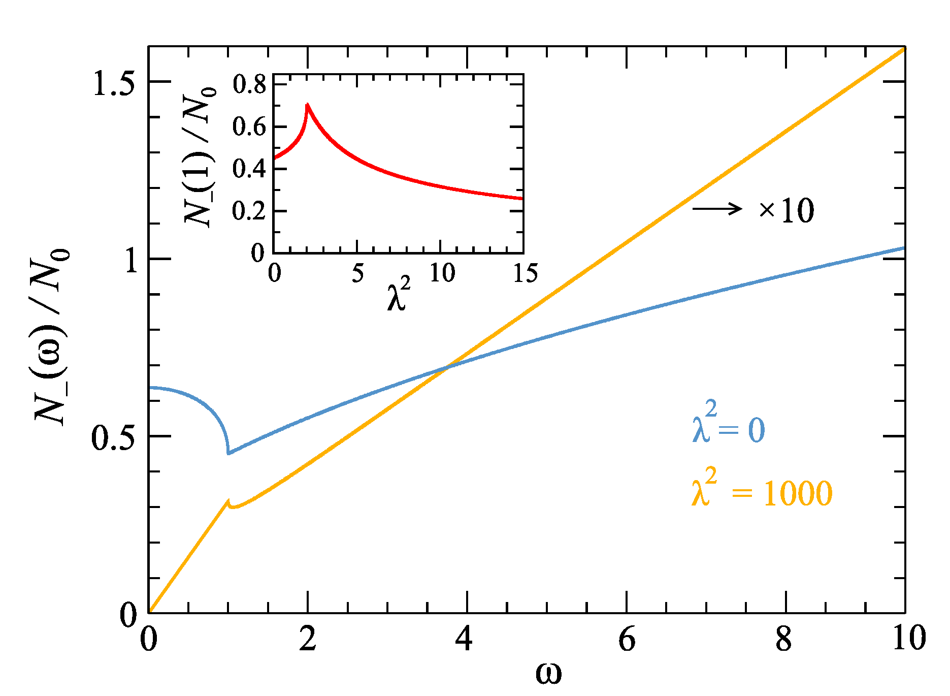
The constraints on $\omega$ and $\lambda$ in (12) appear in terms of the Heaviside $\Theta$-functions in Equation (15). Also notice that, for $\lambda >\sqrt{2}$, the third contribution vanishes. The DOS (15) is shown in Figure 5 as a function of $\omega$ for several values of parameter $\lambda$.

Figure 5. Density of states of the nodal semimetal ($\nu =-1$) with energy dispersion Equation (3) as a function of scaled energy ($\omega$). (a) DOS in the case of self-intersecting spindle phase, appearing for $\lambda <\sqrt{2}$, shown for several values $\lambda$. (b) DOS in the torus phase of the nodal system, appearing for $\lambda >\sqrt{2}$, shown for several values $\lambda$. Black dashed curve in each graph depicts the separatrix, $\lambda =\sqrt{2}$, between regimes (a,b).

Also, in the vicinity of high symmetry points, we expand Equation (15) using the approximative Taylor expansion for $x\ll 1$,

$$\mathrm{Arccos}\left[\pm (1-x)\right]\approx (1\mp 1)\frac{\pi }{2}\pm \sqrt{2x}.$$

(17)

First, we analyze the intersecting spindle case, for $\lambda <\sqrt{2}$ (Figure 5a). The $N_{-}(\omega ,\lambda <\sqrt{2})=N_0\omega /\lambda$ function is linear in $\omega$ from $\omega =0$ up to $\omega ={\omega }_T$, where the van Hove singularity, due to presence of the saddle point in spectrum, is located. The DOS at this point is $N_{-}({\omega }_T,\lambda )=N_0{\omega }_T/\lambda$ while, for $\omega$ just above ${\omega }_T$, Equation (15) can be expanded to

$$N_{-}(\omega ⪆{\omega }_T,\lambda <\sqrt{2})\approx N_0\sqrt{1-\frac{{\lambda }^2}{4}}\left[1-\frac{1}{\pi }\sqrt{\frac{8}{\lambda }}{\left(\frac{1+{\lambda }^2/2}{1-{\lambda }^2/2}\right)}^{1/4}\sqrt{\omega -{\omega }_T}\right].$$

(18)

For $\omega >{\omega }_T$, DOS monotonically decreases until the next van Hove singularity, due to the presence of the elliptic point in spectrum at $\omega =1$, is reached. Since $\omega =1$ is a limiting point that divides two-surfaced and a single-surfaced FS, we inspect, in detail the corresponding DOS. Inserting $\omega =1$ in Equation (15), we obtain

$$N_{-}(\omega =1,\lambda )=\frac{N_0}{\lambda }\left[1-\frac{1}{\pi }\mathrm{Arccos}\left(\frac{{\lambda }^2}{2}-\left|1-\frac{{\lambda }^2}{2}\right|\right)\right].$$

(19)

Equation (19) is shown in Figure 6 (inset). For $\lambda <\sqrt{2}$, it increases as function of $\lambda$, forming a cusp for $\lambda =\sqrt{2}$, after which it decreases as $N_{-}(\omega =1,\lambda >\sqrt{2})=N_0/\lambda$.

Figure 6. DOS in the NLP phase for two special cases: (1) $\lambda \gg 1$ & $\lambda \gg \omega$, according to Equation (23); (2) $\lambda =0$, according to Equation (26). The inset shows DOS taken at the “critical point” $\omega =1$, depending on parameter ${\lambda }^2$, according to Equation (19).

In the high-energy limit, $\omega \gg 1$, only the first two terms in Equation (15) remain. Expanding ${\psi }_{-}^{-}(\omega \gg \lambda ,\lambda )/\omega \approx {\lambda }^2(\omega -P_{-}\left(\lambda \right)/{\lambda }^2)/\left(2{\omega }^2\right)-1$ and using expansion (17), we obtain

$$N_{-}(\omega \gg 1,\lambda <\sqrt{2})\approx \frac{N_0}{\pi }\sqrt{\omega -\frac{P_{-}\left(\lambda \right)}{{\lambda }^2}}\sim \sqrt{\omega }.$$

(20)

Equation (20) is similar to the DOS of the 3D free electron gas. This result is to be expected since, for large wave vectors (i.e., the large energy), the dispersion (3) becomes roughly parabolic in the wave vector since the ${\kappa }^4$ term dominates over the ${\kappa }_z^2$ term.

Some results, found for DOS in the case of intersecting torus, apply for the “doughnut torus” case, $\lambda >\sqrt{2}$. The third term in Equation (15) vanishes, and what remains is DOS linear in $\omega$, i.e., $N_{-}(\omega ,\lambda >\sqrt{2})=N_0\omega /\lambda$, for $\omega <1$. For $\omega =1$, DOS has a discontinuity, as shown by Equation (19), and, just above $\omega =1$, it has a square root dependence,

$$N_{-}(\omega ⪆1,\lambda >\sqrt{2})\approx \frac{N_0}{\lambda }\left[1-\frac{1}{\pi }\sqrt{\frac{2{\lambda }^2}{{\lambda }^2-2}}\sqrt{\omega -1}\right],$$

(21)

which diverges for $\lambda =\sqrt{2}$ and therefore signals that additional elements have to be retained in the expansion of ${\psi }_{-}^{-}(\omega ,\lambda )$. Thus, for $\lambda =\sqrt{2}$, the result up to the leading order in $\omega$ is

$$N_{-}(\omega ⪆1,\lambda =\sqrt{2})\approx \frac{N_0}{\sqrt{2}}\left[1-\frac{2^{3/4}}{\pi }{(\omega -1)}^{1/4}\right],$$

(22)

where it is worth noticing the analytical property that DOS depends on the forth root of energy, appearing only in this case. Finally, in the high-energy limit, $N_{-}(\omega \gg 1,\lambda >\sqrt{2})$ follows the square root dependence given by Equation (20).

We also single out two specific cases:

1. The first one is for energy $\omega$ that satisfies inequality $\lambda \gg 1$ & $\lambda \gg \omega$. It is shown in Figure 6, the ${\lambda }^2=1000$ case. In this interval, the auxiliary function ${\psi }_{-}^{-}(\lambda \gg \omega )\to 0$, so the Equation (15) reduces to

$$\begin{array}{c}\hfill N_{-}(\lambda \gg \omega ,\lambda \gg 1)\approx N_0\frac{\omega }{\lambda }\times \left\{\begin{array}{c}1,\omega <1\hfill \\ 1/2,\omega >1.\hfill \end{array}\right.\end{array}$$

(23)

DOS in this case is linear in $\omega$, with different slopes below and above $\omega =1$, and it is highly reduced in amplitude. This property of linearity, especially in the $\omega >1$ case, is particularly noticeable for the small parameter $\Delta$ in Equation (2) if other bands are much higher (lower) in energy compared to $\Delta$. In this limit, this 3D system effectively resembles the 2D behavior (see the results for DOS in Ref. [21]).

2. The second specific case is for $\lambda =0$. It is a case when Hamiltonian (1) is given only by the first term featuring the ${\sigma }_z$ Pauli matrix. Diagonalization leads to energies

$${\omega }_{\kappa }^{\pm }=\pm \left|1-{\kappa }^2\right|.$$

(24)

Although trivial in appearance, dispersion (24) leads to the unique properties of the corresponding DOS. To see them, we analyze Equation (15), in which the third term can be written as

$$\mathrm{Arccos}\frac{{\psi }_{+}^{-}(\omega ,\lambda )}{\omega }-\mathrm{Arccos}\frac{{\psi }_{-}^{-}(\omega ,\lambda )}{\omega }=\mathrm{Arccos}\left(\frac{{\lambda }^2}{{\omega }^2}\left(1+\sqrt{1-{\omega }^2}\right)-1\right).$$

(25)

Setting the $\lambda \to 0$ in the above expression and using expansion (17) together with Equation (20) in which ${lim}_{\lambda \to 0}{P}_{-}\left(\lambda \right)/{\lambda }^2=-1$, we obtain

$$N_{-}(\omega ,\lambda =0)=\frac{N_0}{\pi }\left[\left(\sqrt{1+\omega }+\sqrt{1-\omega }\right)\Theta (1-\omega )+\sqrt{1+\omega }\Theta (\omega -1)\right].$$

(26)

This special form of DOS is shown in Figure 6 with the dome-like feature for $\omega$ below 1. This can be seen as a natural limit of the trend shown in Figure 5 as $\lambda$ is decreasing.

6. Density of States in the Gapped Phase

Here, we investigate the DOS of the gapped phase by setting $\nu =+1$ in the restrictions enumerated in Section 4, obtaining permitted intervals of u-integration for each case:

➀

$u\in [0,\infty ⟩$,

➂

$u\in [-1-\omega ,-1+\omega ]$,

➂

$u\in ⟨-\infty ,1-{\psi }_{+}^{+}(\omega ,\lambda )]\cup [1-{\psi }_{-}^{+}(\omega ,\lambda ),\infty ⟩$.

In the conditions above, an auxiliary function (11) is implemented and the intersection $u\in ➀\cap ➁\cap ➂$ determines the integration boundaries. We remind the reader that in the GP, $\omega >1$ (i.e., the band is located above the band gap), which makes the integration boundaries easy to determine:

$$\begin{array}{c}\hfill u\in [1-{\psi }_{-}^{+}(\omega ,\lambda ),-1+\omega ].\end{array}$$

(27)

Inserting the integration boundaries (27) in (10), and using (13) and (14), we obtain DOS in the GP phase,

$$N_{+}(\omega ,\lambda )=N_0\frac{\omega }{\lambda }\left[1-\frac{1}{\pi }\mathrm{Arccos}\frac{{\psi }_{-}^{+}(\omega ,\lambda )}{\omega }\right]\Theta (\omega -1),$$

(28)

shown in Figure 7. As in the NLP case, we can determine the limiting values.

Figure 7. Density of states in the gapped phase ($\nu =+1$) of the system, with energy dispersion Equation (3) as a function of scaled energy $\omega$, for different values of parameter $\lambda$, according to Equation (28).

First, by expanding the expression (28) for energies just above the band gap, i.e., $\omega ⪆1$, we obtain

$$N_{+}(\omega ⪆1,\lambda )\approx \frac{N_0}{\pi \sqrt{1+{\lambda }^2/2}}\sqrt{\omega -1}\Theta (\omega -1).$$

(29)

Second, in the high energy limit, $\omega \gg \lambda \approx 1$, similarly to Equation (20), we obtain

$$N_{+}(\omega \gg 1,\lambda )\approx \frac{N_0}{\pi }\sqrt{\omega -\frac{P_{+}\left(\lambda \right)}{{\lambda }^2}}\sim \sqrt{\omega }.$$

(30)

The “square root behavior” in both cases, resembling the 3D free electron gas, is not surprising since we work with the band with the elliptic point at its bottom.

Third, in the case of energies over which the parameter $\lambda$ is the dominant variable, i.e., $\lambda >\omega$, by setting ${\psi }_{-}^{+}(\omega ,\lambda )\to 0$ we obtain

$$N_{+}(\omega >1,\lambda \gg \omega )\approx N_0\frac{\omega }{2\lambda }.$$

(31)

As expected, this is the same result as in Equation (23) (see Figure 7, case $\lambda =10$), which follows from the correct expansion of Equation (3) with dominant $\lambda$-term.

Finally, let us examine the $\lambda \to 0$ limit, in which the expression (29) reduces to

$$N_{+}(\omega ,\lambda =0)=\frac{N_0}{\pi }\sqrt{\omega -1}\Theta (\omega -1),$$

(32)

which is a DOS of the 3D parabolic insulator.

7. Conclusions

We present analytical results comprising electron bands and density of states (DOS) for the effective low-energy two-band electron Hamiltonian, which models the so-called nodal-loop phase (NLP) and the gapped phase (GP) depending on parameters. This way to model the real materials is quite common and useful for the description of the response to the low-energy excitations, the most common among them being the different types of transport properties, such as optical conductivity, for systems with two bands close to the Fermi energy. Besides in the common models, where the density of state naturally appears, such as the plasmon properties, Coulomb screening, or superconductivity mechanisms, it has recently been shown that it plays a key role in the description of the dynamical charge transport in the Holstein-like systems in which it turns out that electron relaxation can be described solely in terms of electron DOS [22]. In that sense, an analytical character of DOS, presented in this paper for the considered Hamiltonian, is of an utmost importance in order to understand the underlying mechanisms leading to the properties of the above-mentioned quantities depending on it.

In this paper, we present analysis of exactly those features. We observe a vanishing value of DOS at the Fermi energy (in the intrinsic case), followed by the linear increase with energy in the NLP case, typical for semimetalic systems, or square-root behavior above the bottom of the band in the GP case, characteristic for 3D insulators with parabolic electron dispersion. Also, we provide a detailed description of DOS around the van Hove singularities appearing due to the presence of the peculiar points in the electron spectrum. In the NLP case, the hyperbolic (saddle) point and the elliptic point are encountered, while the GP case features only the elliptical point at the bottom of the band. A good analysis of similar Hamiltonian with the NLP, from its topological properties to the real materials described by it, is given in Refs. [1,23]. On the other hand, an example of the application of the NLP Hamiltonian to the description of the optical conductivity is given in Refs. [24,25]. The band structure of the corresponding real systems can be quite complex and is usually addressed by different ab initio methods [18,19]. This work intends to complement those methods via the precise, analytical description of the bands and DOS properties in the most relevant region—the narrow interval around the Fermi energy located either in the vicinity of the nodal line or the band gap. The validity of the presented model is closely related to the validity of the effective Hamiltonian (1) in the sense of its deviation from the particular real system, as well as to the nature of an effect one wants to describe. For example, the optical excitations (“vertical transitions”) are very suitable in that matter. Although the presented model is primarily intended to be an analytical tool to help describe and understand features in a number of quantities depending on DOS, we need to at least discuss its experimental observability. The direct experimental observation of DOS is achieved by measuring the Pauli susceptibility, which, on the other hand, requires the doping mechanism to vary the Fermi energy, leaving the bands intact in the process. In other techniques, such as STM and ARPES, DOS appears within the convolution, leading to the specific, technique-dependent response function, and is not directly observable as is. The description of those techniques and corresponding response functions is far out of the scope and main message of this paper and will be discussed elsewhere.