Article

Optimizing Connectivity and Coverage for Millimeter-Wave-Based Networks

by
Pablo Adasme
1,*,
Ali Dehghan Firoozabadi
2,* and
Sergio Cordero
1
1
Centre for Multidisciplinary Research in Telecommunication Technologies (CIMTT), Department of Electrical Engineering, Faculty of Engineering, Universidad de Santiago de Chile, Avenida Víctor Jara 3519, Estación Central, Santiago 7800002, Chile
2
Department of Electricity, Universidad Tecnológica Metropolitana, Av. Jose Pedro Alessandri 1242, Santiago 7800002, Chile
*
Authors to whom correspondence should be addressed.
Symmetry 2024, 16(1), 123; https://doi.org/10.3390/sym16010123
Submission received: 29 December 2023 / Revised: 12 January 2024 / Accepted: 16 January 2024 / Published: 19 January 2024

Abstract

:
In this article, the problem of achieving the minimum backbone connectivity cost while simultaneously maximizing user coverage for 5G millimeter-wave (mmWave)-based networks is considered. Let G = ( N , E ) be an input graph instance with a set of nodes N (base stations) and a set of edges E. It is assumed that G represents a wireless backbone network. Let M represent a set of users to be covered by G. Note that mmWave technology has been considered in the literature as an important candidate solution for 5G networks due to its low latency. However, there remain some problems to be addressed before using this technology. A serious one is that millimeter waves cannot cover large transmission distances. In this article, the proposed methodology consists of formulating mixed-integer programming models to deal with the problem from a management point of view. Our models allow the determination of which of the nodes of G should be active and connected while simultaneously maximizing the total number of covered users. The models are solved with the CPLEX solver using its branch and cut and automatic Benders decomposition algorithms. For this purpose, symmetric complete and sparse graphs are considered. Using the symmetry concept, it is considered that the distances between base stations and users and between base stations themselves are symmetrical. Finally, an efficient local search meta-heuristic is proposed that allows for finding near-optimal solutions. Our numerical experiments indicate that the problem is hard to solve optimally. Thus, instances with up to 40 nodes and 500 users have been solved to optimality so far. In particular, it is observed that one of the models presents slightly better performance in terms of CPU time. Finally, the heuristic approach allows us to obtain tight solutions with less computational effort when dealing with even larger instances of the problem.

1. Introduction

Using 5G technology for wireless communication can make it easier to send a lot of data quickly. It has the potential to overcome problems like limited bandwidth, access issues, and delays. This means that future technologies, like “5G and Beyond”, could let us send data at speeds of hundreds of Megabits per second with very short delays, less than 1 millisecond. As a consequence, it will make it possible to connect simultaneously billions of devices and it can also lead to the creation of entirely new and innovative applications that we haven’t seen before [1]. Examples of where these new applications could be used cover a wide range of areas. This includes things like mobile health, self-driving cars, manufacturing and entertainment, education, smart grids, big data analysis, smart cities and homes, aerospace, ocean exploration, emergency response, and mobile platforms, among others [1]. As can be verified from the literature, a base station (BS) can transmit data with up to a radius of approximately 200ms while using 5G mmWave technology [2]. So far, the experimental evidence suggests that deploying base stations (BSs) with a radius of at least 200 m can solve the coverage issue in outdoor areas by utilizing direct line-of-sight communication. However, it is important to note that opting for smaller radius values would mean needing a significantly larger number of base stations to ensure complete coverage for users [2,3]. In particular, note that any pair of BSs can be connected by using cables to form the backbone network structure. Consequently, it is necessary to adapt current infrastructures [4]. This will be essential for the deployment of future 5G-based networks to manage the increasing demand for data usage and broader coverage, as recommended in [2,5].
In this article, the problem of achieving the minimum backbone connectivity cost while simultaneously maximizing user coverage using 5G mmWave technology is considered. For this purpose, let us consider G = ( N , E ) to be an input graph instance with a set of nodes (BSs) N = { 1 , , n } and a set of edges (or connection links) E = { { i , j } i , j N , ( i < j ) } . Thus, it is assumed that G represents a wired or wireless backbone network. Also, let M = { 1 , , m } represent a set of users to be covered by G. Note that mmWave technology has been considered in the literature as an important candidate solution for 5G networks due to its low latency. Nevertheless, there remain some practical problems to overcome before using this technology for real network applications. A serious one is that millimeter waves cannot cover large radial transmission distances. Consequently, in this article, the main contributions are to propose mixed-integer programming models to deal with this problem. In particular, our models allow the determination of which of the nodes of G should be active and connected at the lowest connectivity cost while simultaneously maximizing the total number of covered users. More precisely, two flow-based models, a Miller–Tucker–Zemlin-based one and an exponential one, are proposed [6]. In general, these models mainly differ in the way a set of constraints forms a spanning tree backbone. In our research article, we consider scenarios where network nodes remain stationary, which is a common characteristic of sensor networks, for instance, or in catastrophic scenarios where it might be required to set up a wireless network communication rapidly, such as in earthquakes or pandemic situations. If a particular user is not covered, they will disconnect from the backbone network, as occurs, for example, on rural highways. This underpins our assertion that the novel models we introduce have direct applicability to wireless networks. This assumption aligns well with the prevalent conditions in sensor network deployments. However, we recognize the more intricate scenario involving mobile BSs and users, capable of traversing various application domains. Note that even in dynamic scenarios, our proposed models retain their utility, offering an alternative avenue to derive optimal network configurations. This optimization task is facilitated by considering optimization tools such as the CPLEX solver, an industry-leading solution in the realm of operations research [7]. Its efficacy is underscored by its inclusion of exact approaches like branch and cut (B&C) and Benders algorithms, aspects well-documented in the literature [7,8]. Within the context of wireless sensor networks (WSNs), a myriad of applications has been explored in the existing body of work. It is also observed that additional metrics such as users’ and BS’s mobility, quality of service requisites, and security provisions will certainly lead to future modeling approaches. Nevertheless, our models and algorithms address the pivotal issue of distance—both between BSs and users and among BSs themselves. This treatment is rooted in the understanding that many metrics are contingent on distance, often exhibiting degradation as distances increase. Note that even when both BSs and users are in motion, our models and algorithms remain efficient, consistently yielding near-optimal solutions remarkably, as demonstrated through our numerical experiments. This adaptability positions them not only as practical tools but also as a benchmark for the development of novel and more efficient algorithmic approaches. While they may not be amenable to exact solutions within a one-hour CPU time limit in certain cases, the extensive use of rigorous upper and lower bounds ensures that the solutions attained are indeed near-optimal. Our contribution, therefore, lies not just in the solutions themselves but in the robust methodology employed to ascertain their quality. In summary, the contributions outlined in our novel models exhibit a remarkable degree of generality, making them adaptable to a range of contexts, contingent upon the specific application domain. This flexibility underscores their value as a versatile toolset for addressing diverse wireless network scenarios. Finally, in a situation where the BSs and users move, there are always alternative ways of finding feasible solutions faster. For this purpose, our second algorithm uses an iteration parameter MaxIter which allows it to run for a predefined number of iterations. The latter can be handled efficiently to find good solutions, as is seen from the velocities reported in the last two figures, where the algorithm reaches near-objective values very fast. Since all our models are solved with the CPLEX solver using its branch and cut and its automatic Bender decomposition algorithmic options, a set of complete and sparse connected input graphs to form the backbone network is considered. So, the assumption is that the positions of all users and base stations BSs are randomly distributed within a square area. Additionally, the assumption is made that in an outdoor setting, all users and base stations BSs can communicate using a direct line-of-sight channel. For this purpose, the maximum CPU time limit allowed for the CPLEX solver is arbitrarily set to be at most one hour when solving each of the instances, and also the CPLEX Mipgap option is set to be zero and less than one percent [7]. Finally, an efficient local search meta-heuristic algorithm is proposed that allows for finding tight solutions in significantly low CPU time when compared to the proposed models either for small- or large-sized instances of the problem. As far as we know, our proposed models and solution approaches are new to the literature and therefore enrich the existing literature to deal with the problem from a management point of view. Note that our proposed models allow us to incorporate a new aspect to the problem which is considering the distance between users and base stations BSs, and the optimal connectivity between all BSs. Finally, we mention that our proposed models could cover all users when the maximum user coverage metric becomes more relevant than considering the connectivity cost of the backbone network. Total coverage could also be ensured by using a larger amount of candidate sites for the BSs to be activated in the network.
Consequently, a direct comparison with other methods is not straightforward as the modeling and algorithmic approaches are completely new. From the literature, only one article was found to be as close as possible to the connectivity problem, where a flow-based formulation is proposed. In this article, that flow model is adapted to our new more intricate problem. Unfortunately, its performance in terms of obtaining optimal solutions when compared to our new proposed models is poor. Moreover, all our proposed models allow us to determine the optimal number of BSs and which of them should be active to form the backbone network structure. This consideration also takes into account the characteristics of 5G mmWave technology. It is worth noting that the literature has not yet explored the aspect of wireless networks with random deployments, such as sensor networks. Note that the rationale behind employing the CPLEX solver primarily rests on its exceptional, unique, and potent algorithmic capabilities, as evidenced by its success in tackling challenging optimization problems in the literature [7]. Finally, we mention that this work corresponds to a larger version of the article presented at the IEEE conference [9].
The organization of the article is as follows. In Section 2, first, some recent studies from the literature that are closer to the optimal network planning problem considered in this article are reviewed. Then, in Section 3, the optimization problem at hand is briefly explained, and each proposed mathematical formulation is presented in detail. Subsequently, in 
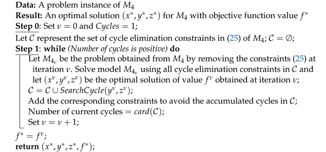
Section 4, the algorithmic approaches used to solve the optimization problem are presented and explained. More precisely, an exact algorithm that consists of adding sub-tour elimination constraints to our exponential model until the optimal solution is obtained without cycles is presented. Then, how the Bender decomposition algorithm finds the optimal solutions and the automatic Benders CPLEX version as well are briefly explained [
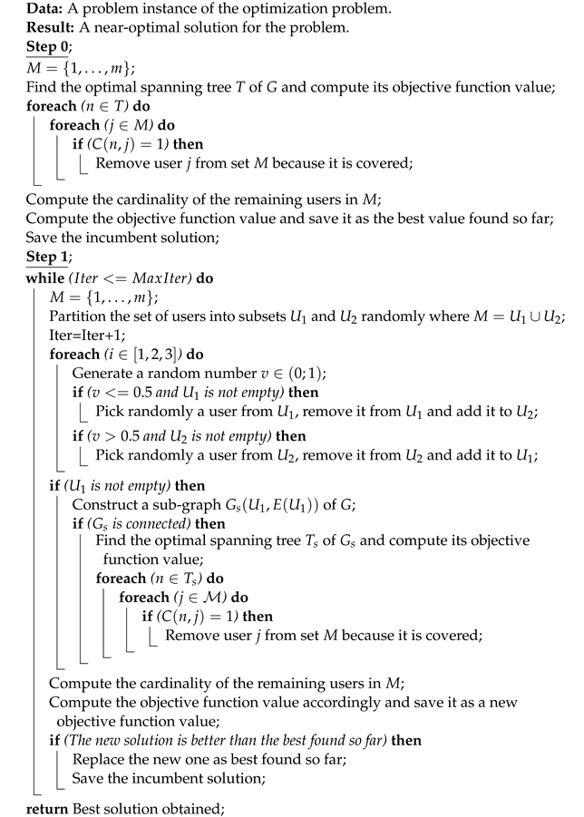
7]. Finally, in this section, we introduce and clarify the proposed meta-heuristic. Moving forward to Section 5, we carry out extensive numerical experiments, presenting and discussing the results obtained from the proposed models and algorithms. The comparison is based on factors such as CPU time and the optimal or best solutions achieved. Lastly, in Section 6, we conclude the article while discussing insights for potential future research.

2. Related Work

The BS placement problem using 5G mmWaves for outdoor areas has not been investigated so far with sufficient depth in the literature. Some recently published works using mmWaves technology which are closely related to this network planning problem can be described as follows. In [10], the authors utilize mmWave radar technology to unobtrusively detect human falls. To this end, they collect data from healthy young volunteers with the radar mounted on the side wall or overhead of an experimental room. They consider a set of features that are manually extracted from the data and apply multilayer perceptron, random forest, k-nearest neighbor, and support vector machine classifiers on the features. Subsequently, they devise a convolutional neural network and conclude from their numerical results that the development of a hidden monitoring system for fall detection using mmWave radar is feasible. Finally, the authors mention that the optimal placement of the radars is unknown, and consequently, they locate them intuitively. Similarly, in [11], the authors propose a novel 3D geometry-based framework for deploying mmWave base stations in urban environments and also provide a solution for the optimum deployment of passive metallic reflectors to extend the radial coverage to non-line-of-sight areas. Specifically, they formulate their network planning problem as two independent optimization problems to maximize the coverage area, and minimize the deployment cost, while ensuring a desired quality-of-service level. Finally, they test the efficacy of their approach by using a generic map. The study conducted by the authors concludes that their network planning approach, utilizing mmWave technology, effectively reduces the need for passive metallic reflectors in non-line-of-sight areas, consequently lowering deployment costs. In [12], the authors investigate the practicality of relaying and caching in mmWave-based networks, assuming the coexistence of base stations and relay nodes (RNs). Their findings suggest that increasing the number of RNs and expanding the cache size in mmWave networks presents a more cost-effective solution compared to simply increasing BS density for similar backhaul off-loading performance. Another work [13], explores advanced computational geometry concepts for placing numerous mmWave wall-mounted BSs in large urban areas. The authors assert that their study is the first to use mmWave cells on buildings, and their approach enables accurate modeling for small-cell mmWave-based networks, providing gigabit capacities for densely populated urban areas.
In addition to the mentioned works, recent publications on network planning issues for future communication networks include references [6,14]. In the specific case of [14], the authors tackle the broader challenge of maximizing user coverage while adhering to facility location and radial distance constraints in the context of 5G/6G wireless communication networks. They propose mixed-integer linear programming models, drawing inspiration from the classical p-median problem in optimization literature. Notably, the authors introduce non-overlapping radial distance constraints for various pairs of base stations (BSs). Their experiments involve solving instances with up to 100 antennas and 1000 users. The study concludes that incorporating a larger number of radius values enhances the flexibility and accuracy of solutions, albeit at a higher computational cost. In a similar vein, in [6] the author proposes generic and novel mixed-integer linear programming models for the p-median problem while imposing ring, tree, and star backbone topology constraints on the facility locations. The author also mentions that the proposed models find applications in wired and wireless network design, computer networks, transportation, water supply, and electrical networks, to name a few. The author further proposes a variable neighborhood search meta-heuristic for each network backbone structure. Finally, the author concludes, based on substantial numerical experiments, that the ring models are harder to solve with CPLEX than the tree and star ones. Ultimately, the proposed meta-heuristics in [6] proved to be highly efficient as they allowed better feasible solutions to be obtained compared to CPLEX, and with significantly less computational effort. Other related works can be consulted in references [2,15,16] and in references therein. As can be observed from these previous works, none of them takes into account the radial transmission distance limitation of 5G mmWave technology so far. Consequently, the proposed mathematical models in this article change in structure significantly to deal with the network planning problem from a management point of view.
To conclude this section, it is mentioned that we observe only a few works in the literature that are directly related to the network planning problem using 5G mmWave technology. Consequently, our work will contribute to providing a new dimension of the problem, i.e., taking into account optimal connectivity. Since the objective function of our proposed models contains conflicting objectives, i.e., maximizing user coverage and minimizing backbone connectivity cost simultaneously, a weighting parameter α [ 0 ; 1 ] is introduced to balance the degree of importance of each objective. Finally, it is mentioned that the direct implication for the mmWave networks is to at least find very good solutions, including optimal configurations.

3. Optimization Problem and Mathematical Formulations

In this section, first, the optimization network planning problem we are dealing with is introduced. For this purpose, an example of an input graph network and the optimal solution obtained is presented. Subsequently, each proposed model is presented and explained in detail.

3.1. Optimization Problem

As mentioned in Section 1, a network deployment that is composed of users and BSs that are randomly located inside a square area of 1 km 2 is considered. It is also assumed that each user can connect to at least one BS located within a predefined radial transmission symmetric distance. For this purpose, it is assumed that the distances between base stations and users and between base stations themselves are symmetric. Thus, the main goal is to cover the maximum number of users in the network with at least one of the BS (nodes) while simultaneously minimizing the total connectivity cost of the BSs. In particular, the main focus is put on the context of 5G mmWave since it is assumed that the distances between users and BSs are particularly small. Note that the latter implies using a larger number of BSs to cover the entire network.
In Figure 1 and Figure 2, the input backbone network together with the optimal solutions, one for a sparse graph and another one for a complete graph, are presented. Note that the input graphs are given as digraphs as they will be required to solve the proposed models, whereas the optimal backbone solutions are drawn employing undirected graphs. The digraph version of each undirected input graph is, thus, denoted hereafter by H = ( N , A ) , where A represents a set of directed arcs, i.e., the set E = { { i , j } i , j N , ( i < j ) } is transformed into the set A = { ( i , j ) i , j N , ( i j ) } . Note that the arcs obtained in the optimal solutions can be simply dropped and replaced by edges instead. As can be seen in Figure 1, the input backbone network is connected. It is also seen that eight nodes of the optimal solution obtained are active and connected while forming a tree backbone topology. Only two BSs are not included in the solution. This means that the maximum number of covered users, which is 30 out of 50 for the example of Figure 1, can connect with at least one of the active nodes. Similarly, from Figure 2, it is observed that two BSs are not part of the optimal solution, and thus, not required to cover users. In this example, the number of covered users is 27 out of 50.

3.2. Mathematical Formulations

To formulate a first mixed-integer linear flow-based model, let M = { 1 , , m } and N = { 1 , , n } denote the corresponding sets of users and BSs, respectively. The binary variable x j for each user j M equals one when user j is covered by some of the active BSs, otherwise x j = 0 . Subsequently, the binary variable y i should be equal to one if BS i N is active, otherwise y i = 0 . Consequently, the first linear flow-based model for the 5G mm-Wave-based network, which is denoted hereafter by M 1 , consists of maximizing the total number of covered users while simultaneously minimizing the total backbone connectivity cost of the active BSs. The model can be written as follows:
M 1 : max { x , y , z , f } α j M x j ( 1 α ) ( i , j ) A D i j z i j
s t : i N C i j y i x j , j M
( i , j ) A z i j = i N y i 1
j ( r , j ) A r z r j = 1  
j ( r , j ) A r f r j = i N y i
i ( i , j ) A A r f i j i ( j , i ) A f j i = y j , j N
f i j n z i j , ( i , j ) A A r
z i j + z j i 1 , ( i , j ) A
f i j n y i , ( i , j ) A
f i j n y j , ( i , j ) A
x { 0 ; 1 } m , y { 0 ; 1 } n , z { 0 ; 1 } A A r ,
f [ 0 ; ) A A r
In model M 1 , the variable z i j for all ( i , j ) A equals one if the connection link between nodes i and j N are part of the backbone, otherwise it equals zero. Similarly, the non-negative variable f i j for all ( i , j ) A A r can take positive values if and only if variable z i j = 1 , otherwise f i j should be equal to zero. For this purpose, it is considered an expanded digraph of G = ( N , E ) , as H = ( N r , A A r ) , where the set of nodes in H considers an additional dummy node r and a set of arcs A r composed of the arcs in A plus additional arcs with zero costs going from r to every node j N . Next, in the objective function (1), the parameter α [ 0 ; 1 ] represents a weighting parameter that balances the degree of importance of each term. Each entry in the input matrix C = ( C i j ) , for all i N , j M is a 0–1 value indicating whether user j is covered or not by BS i. In particular, note that it is possible to compute each of these entries by imposing a predefined radial transmission distance. If the distance of BS i N reaches user j M , then C i j = 1 ; otherwise, C i j = 0 . On the other side, each entry in the input matrix D = ( D i j ) denotes the existing distance between BSs i and j N .
Observation 1.
Note that when α = 1 in the objective function (1), the model M 1 reduces only to maximizing the total sum of covered users without taking into account the connectivity costs between BSs. On the other hand, when α = 0 the output solution of the problem reduces to a trivial minimum-cost spanning tree. Furthermore, note that the solution-spanning tree to be obtained will be composed of one isolated node with an objective function value equal to zero.
Thus, the underlying idea of using parameter α [ 0 ; 1 ] is to find the maximum possible number of covered users while simultaneously connecting a spanning tree backbone of minimum cost which is formed with the active BSs. Note that distances are used for each entry in the input matrix D = ( D i j ) for all i and j N in (1). As a commonly recognized fact, the signal quality experiences a notable improvement with the transmission distance in a wireless communication channel. In simpler terms, when the emitter and receivers are in closer proximity, the power consumption tends to be lower, as highlighted in the study by [6].
Constraints (2) allow a particular user j M to be covered if and only if at least one of the BSs is active and the user is located inside its sensing radius. Next, constraint (3) ensures that the backbone spanning tree obtained contains several edges equal to the number of nodes minus one. Constraint (4) ensures that only one arc goes from r to a unique node j N . Subsequently, constraints (5) ensure that an amount of i N y i units of flow enter into the unique arc ( r , j ) of variable z i j , ( i , j ) A A r . Similarly, constraints (6) ensure that one unit of flow equals the incoming total flow minus the outgoing total flow for each active BS. Constraints (7) indicate that at most n units of flow should traverse the arc ( i , j ) A A r if and only if variable z i j = 1 , i.e., if the nodes i and j N are connected. Next, constraints (8) ensure that either arc ( i , j ) or arc ( j , i ) is part of the output solution of the input digraph. Constraints (9) and (10) are valid inequalities forcing the fact that variable f i j cannot be positive if neither i nor j is an active BS. Finally, constraints (11) are domain constraints for the decision variables.
Another equivalent flow-based formulation adapted from [2] can be written as follows:
M 2 : max { x , y , s , f , z , θ } α j M x j ( 1 α ) ( i , j ) A D i j z i j s t : i N C i j y i x j , j M
i N s i = 1
j N ( f j i f i j ) + y i = j N θ i j , i N
θ i j y j , i , j N
θ i j s i , i , j N
θ i j y j + s i 1 , i , j N
f i j n y i , ( i , j ) A
f i j n y j , ( i , j ) A
f i j n z i j , ( i , j ) A
z i j + z j i 1 , ( i , j ) A
x { 0 ; 1 } m , y { 0 ; 1 } n , s { 0 ; 1 } n ,
z { 0 ; 1 } A , θ [ 0 ; 1 ] n 2 , f [ 0 ; ) A
In model M 2 , the variable s i for all i N is used to represent the source node from which j N y j 1 units of flow must traverse the network formed with the active BSs. Otherwise, it equals zero. On the other hand, when s i = 0 , then the incoming minus outgoing flow of node i N must be equal to −1. Note that this fact is simultaneously implied by constraints (12) and (13). Constraints (14)–(16) are standard linearization constraints [17]. More precisely, the binary quadratic products θ i j = s i y j , for all i , j N are linearized with the constraints (14)–(16). Finally, the domain constraints of the decision variables are referenced in (17). The remaining constraints are similar to the ones presented in model M 1 .
A Miller–Tucker–Zemlin-based constrained formulation can also be written as follows [18]:
M 3 : max { x , y , u , z } α j M x j ( 1 α ) ( i , j ) A D i j z i j s t : i N C i j y i x j , j M ( i , j ) A z i j = i N y i 1
u i j N y j , i N
u i y i , i N
i ( i , j ) A z i j y j , j N
u j u i ( n 1 ) z i j ( n 3 ) z j i 2 n , ( i , j ) A
z i j + z j i y i , ( i , j ) A
z i j + z j i y j , ( i , j ) A
x { 0 ; 1 } m , y { 0 ; 1 } n , z { 0 ; 1 } A
where constraints (18)–(21), which are polynomials in number, avoid cycles in the output solution of the problem. Note that, in particular, constraint (20) ensures that each node of the backbone tree has at most one incoming arc. Next, constraints (22) and (23) are valid inequalities forcing the fact that either arc ( i , j ) or ( j , i ) A is equal to one since the input graph is a digraph. And for this purpose, both nodes i and j N must be active, which is reflected by variables y i and y j , respectively.
The last formulation proposed has an exponential number of constraints in (25). More precisely, for each subset S N ,a constraint is imposed that avoids forming a cycle with the nodes belonging to S. The model reads
M 4 : max { x , y , z } α j M x j ( 1 α ) ( i , j ) A D i j z i j s t : i N C i j y i x j , j M
( i , j ) A ( S ) z i j | S | 1 , S N
z i j + z j i y i , ( i , j ) A
z i j + z j i y j , ( i , j ) A
( i , j ) A z i j = i N y i 1
i ( i , j ) A z i j y j , j N
x { 0 ; 1 } m , y { 0 ; 1 } n , z { 0 ; 1 } A
The rest of the constraints are the same as in the above models, thus not labeled. Finally, the domain constraints of the decision variables are written in (26).
We mention that another relevant metric that could be considered as part of future research in the proposed models is the interference between small cells, as pointed out in [5]. It is also possible to consider maximizing the capacity and minimizing power consumption, leading to harder nonconvex nonlinear formulations. Ultimately, note that these metrics can be added as constraints in the optimization models as well.

4. Algorithmic Approaches

In this subsection, the two algorithms are presented and explained. One is exact and consists of adding cycles iteratively to model M 4 until no cycle is obtained in an incumbent solution [19]. The second one is an approximate local search heuristic that is highly efficient as it allows obtaining near-optimal solutions in very short CPU times. Finally, the reader is referred to some relevant references involving the well-known exact methods of branch and cut and Benders decomposition of the CPLEX solver [7].

4.1. Exact Algorithm for Solving Model M 4

The iterative procedure to avoid having cycles in model M 4 consists of ignoring, at the beginning of the algorithm, the exponential number of constraints (25). In other words, first, model M 4 is solved without constraints (25). If an output solution containing cycles is obtained, we find one of the cycles arbitrarily, as there can be many of them, and re-optimize while adding the particular constraint avoiding that particular cycle. Then, Algorithm 1 continues with that iterative process. Note that at a certain iteration one may obtain a solution without cycles: that solution would be the optimal one. The procedure is depicted in Algorithm 1. The method is simple and quite general. Note that any cycle, if it exists, can be detected by a depth-first search procedure [20]. Also, note that the number of constraints in (25) is at most O ( 2 n ) . Consequently, Algorithm 1 converges to the optimal solution of the problem in at most O ( 2 n ) outer iterations (see the proof of theorem 2 in [19]). In step 0, Algorithm 1 initializes the iteration variable ν = 0 and it is assumed that there is at least one cycle to enter the loop. Next, it initializes the set of constraints of type (25) of M 4 . Note that initially this set is empty. Subsequently, in step 1, Algorithm 1 enters the while loop that is broken only if there are no further cycles in the incumbent solution. The inner loop is self-explained, and in particular the method S e a r c h C y c l e ( ) allows for finding a cycle using the depth-first search algorithm [20].
Algorithm 1: Exact iterative algorithm for solving M 4 .
Symmetry 16 00123 i001

4.2. Approximate-Based Local Search Heuristic

Now, the approximate-based local search heuristic, Algorithm 2, is presented and explained. This algorithm allows for obtaining near-optimal solutions in a short CPU time for the optimization problem. The algorithm receives an instance of the problem and returns a near-optimal solution. In particular, in step 0, Algorithm 2 initializes the set M, finds the optimal spanning tree T of G, and computes its objective function value. In the beginning, it performs this using all nodes of the backbone. Then, it counts the number of covered users. The latter is achieved by using matrix C = C ( i , j ) for all i N and for all j M . Subsequently, it calculates the cardinality of the remaining users, i.e., the number of users who are not covered by T. This allows for computing the objective function value and saving it as the best found so far. Finally, the best current solution found is saved. Next, in step 1 it enters into a while loop which is run for a maximum predefined number of iterations M a x I t e r . The process is repeated and inside the loop consists of initializing the set of users M while including all users. Next, it randomly partitions the set of users into two subsets U 1 and U 2 , where M = U 1 U 2 . Next, the algorithm increments by one unit the number of iterations I t e r . Then, it performs the following three times. It randomly generates a number v ( 0 ; 1 ) and asks if v < = 0.5 and U 1 is not empty. If this is the case, it randomly chooses a user from U 1 , removes it from U 1 , and adds it to U 2 . On the other hand, if v > 0.5 and U 2 is not empty, it randomly picks a user from U 2 , removes it from U 2 , and adds it to U 1 . Subsequently, it performs several tasks only if U 1 is not empty. More precisely, first, it constructs a sub-graph G s ( U 1 , E ( U 1 ) ) of G, where the set E ( U 1 ) represents all incident edges to the nodes of U 1 . Then, it asks if the sub-graph G s is connected. If this is the case, it finds the optimal spanning tree T s of G s and computes its objective function value. Next, it counts the set of covered users. The latter is performed for each n T s and j M using matrix C = C ( n , j ) . Subsequently, it computes the cardinality of the remaining users in M and calculates the objective function value according to the new backbone tree T s . If the new solution obtained with T s is better than the best found so far, then it is saved as the best incumbent solution obtained. Finally, when the process ends, the algorithm returns the best solution found.
Algorithm 2: Approximate-based local search heuristic for solving the optimization problem.
Symmetry 16 00123 i002

5. Results and Discussion

In this section, substantial numerical experiments are conducted to compare the performances of the proposed models M 1 , M 2 , M 3 , M 4 , and the proposed algorithms. To this end, a Python code is implemented using the CPLEX solver [7]. In particular, the models M 1 , M 2 , and M 3 are solved with both the branch and cut and the Benders decomposition options of the solver. Note that model M 4 has no continuous variables and, consequently, Benders approach cannot be applied [8]. In particular, for solving the models M 1 , M 2 , and M 3 , the CPLEX solver is used with default options. The maximum CPU time is limited to at most one hour. Consequently, if a particular reported objective value is obtained in 3600 s or more, it means that the solver is reporting the best solution obtained in one hour. Otherwise, it corresponds to an optimal solution to the problem. Note that the optimization problems of this type are NP-hard due to their discrete nature. Thus, both algorithms used by the CPLEX solver have exponential complexity [7]. The numerical experiments were performed on an Intel(R) 64-bit core (TM) i5-8400 CPU 2.81 GHz with 16 G of RAM under Windows 10. Randomly sparse and complete input graphs were generated. In the latter, it was assumed that all active BSs can be connected using cables, for instance. Whilst for the sparse graphs it was assumed that the radial transmission range between BSs was 300 ms. The dimensions of the graphs in terms of the number of nodes and the number of users were N = { 40 ; 60 ; 100 } and M = { 250 ; 500 ; 1000 } , respectively. Finally, it was assumed that each user could connect to an active BS if and only if the user was located inside a radial transmission range of at most 200 ms. Each of the coordinates for the nodes and users was generated within a square area of 1 km 2 according to a uniform distribution function. Thus, each entry of the input distance matrix D was computed using these coordinates.
In Table 1 and Table 2, numerical results are reported for the models M 1 and M 2 , respectively. In particular, Table 1 reports numerical results for the sparse graphs. Whereas Table 2 reports numerical results for the complete ones. In both tables, the legends are the same. In columns 1 and 2, the instance number and the density of the graph are presented. The latter is computed by dividing the number of edges by the total number of edges of a complete graph having the same number of nodes. Column 3 reports the weighing parameter α . Next, columns 4–6 and 7–9 report the best objective value obtained, the number of branch and bound nodes, and the CPU time in seconds for model M 1 when solved with the branch and cut and Benders algorithms, respectively. Similarly, columns 10–12 and 13–15 report the same information for M 2 .
In Table 1, from the sparse graph results, it is mainly observed that, in general, M 1 outperforms M 2 . First, one can note that the best solutions obtained with M 1 are the optimal ones for all the instances when using n = 40 nodes, either using B&C or Benders algorithms. On the other hand, it is observed that M 2 does not optimally solve the instances with the B&C algorithm. However, it can solve all the instances optimally using Benders algorithm. These observations can be confirmed by looking at the columns of the CPU times and the number of branching nodes. Subsequently, one can see that none of the graphs composed of n = 60 nodes can be solved optimally in one hour of CPU time. The latter shows that the graph instances become significantly harder to solve when n grows. Finally, it is observed that for the value of α = 1 , the problem is solved easily with any of the models and methods. In particular, for the complete graph instances reported in Table 2, it is possible to observe similar trends. More precisely, one can see that M 1 can solve all the instances optimally for n = 40 with both methods. It is also observed that none of the instances can be solved optimally in one hour of CPU time for n = 60 nodes. Furthermore, it is observed that M 2 obtains the optimal solutions for all the instances for n = 40 with Benders approach. The latter cannot be achieved with the pure B&C method. Lastly, it is seen that all the graph instances are solved optimally and very rapidly for the value of α = 1 , which is the optimization problem without taking into account the connectivity cost of the backbone. Ultimately, from both Table 1 and Table 2, one can observe that the increase in users, going from 500 to 1000, does not have a significant impact on the performance when solving the problem. In Table 3 and Table 4, numerical results are reported for models M 3 and M 4 . In particular, Table 3 and Table 4 report numerical results for the sparse and complete graphs, respectively. In both tables, the legends are the same. More precisely, in columns 1–3, the instance number, the density of the graph, and the value of the parameter α are presented. Next, columns 4–6 and 7–9 report the best objective function value obtained, the number of branch and bound nodes, and the CPU time in seconds for model M 3 when using the B&C and Benders algorithmic approaches, respectively. Finally, columns 10–13 report the best objective function value obtained with Algorithm 1, the CPU time in seconds required to obtain that solution, the number of iterations of Algorithm 1, and the gap which is obtained by subtracting the best objective value obtained with M 4 with the best objective value obtained with the remaining models and dividing this quotient by the latter value. The gap is finally multiplied by 100 to present percentages. Note that the objective values obtained with models M 1 , M 2 , and M 3 are lower bounds as they are feasible or in the best case optimal solutions, while the values obtained with M 4 are in the best case the optimal solutions or upper bounds since they are solved iteratively without including all sub-tour elimination constraints within each iteration of Algorithm 1.
From Table 3, for the sparse graphs, one can see that M 3 cannot solve any of the instances with a certificate of optimality with any of the algorithms since the CPU time values are larger than one hour. Again, the exception occurs for the graphs using α = 1 , which are easily solved with any of the methods. For M 4 , it is not possible to ensure that the objective values correspond to the optimal solutions because they are not obtained in less than one hour. However, in the case of model M 4 , recall that the objective values are upper bounds. Consequently, one can ensure that the graph instances having zero gaps report the optimal solutions. This is because these upper bounds are equal to the lower bounds obtained with one or more of the remaining models. This also ensures that the lower bounds obtained with the other models correspond to optimal solutions. For the complete graph instances in Table 4, one observes similar trends. One can see that only one graph instance is solved optimally in less than one hour. However, it is again mentioned that for model M 4 the graph instances having zero gaps report the optimal solutions. The argument is the same as for the sparse graphs presented in Table 3, i.e., the upper bounds are equal to the lower bounds.
To conclude, from the numerical results presented in Table 1, Table 2, Table 3 and Table 4 one can mainly observe that model M 1 has a slightly better performance than the rest of the models when using the pure B&C approach of the CPLEX solver, at least for the reported instances.
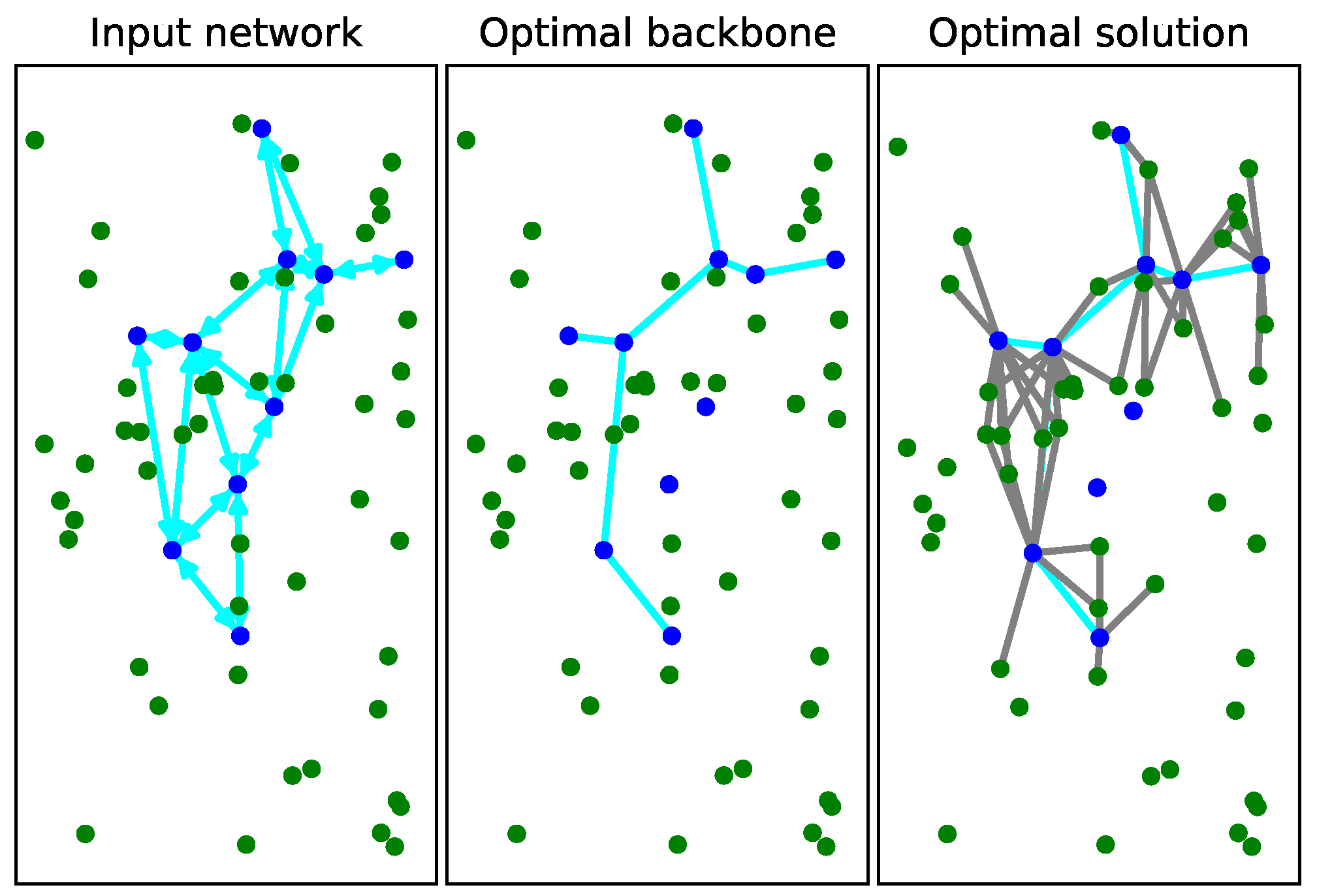
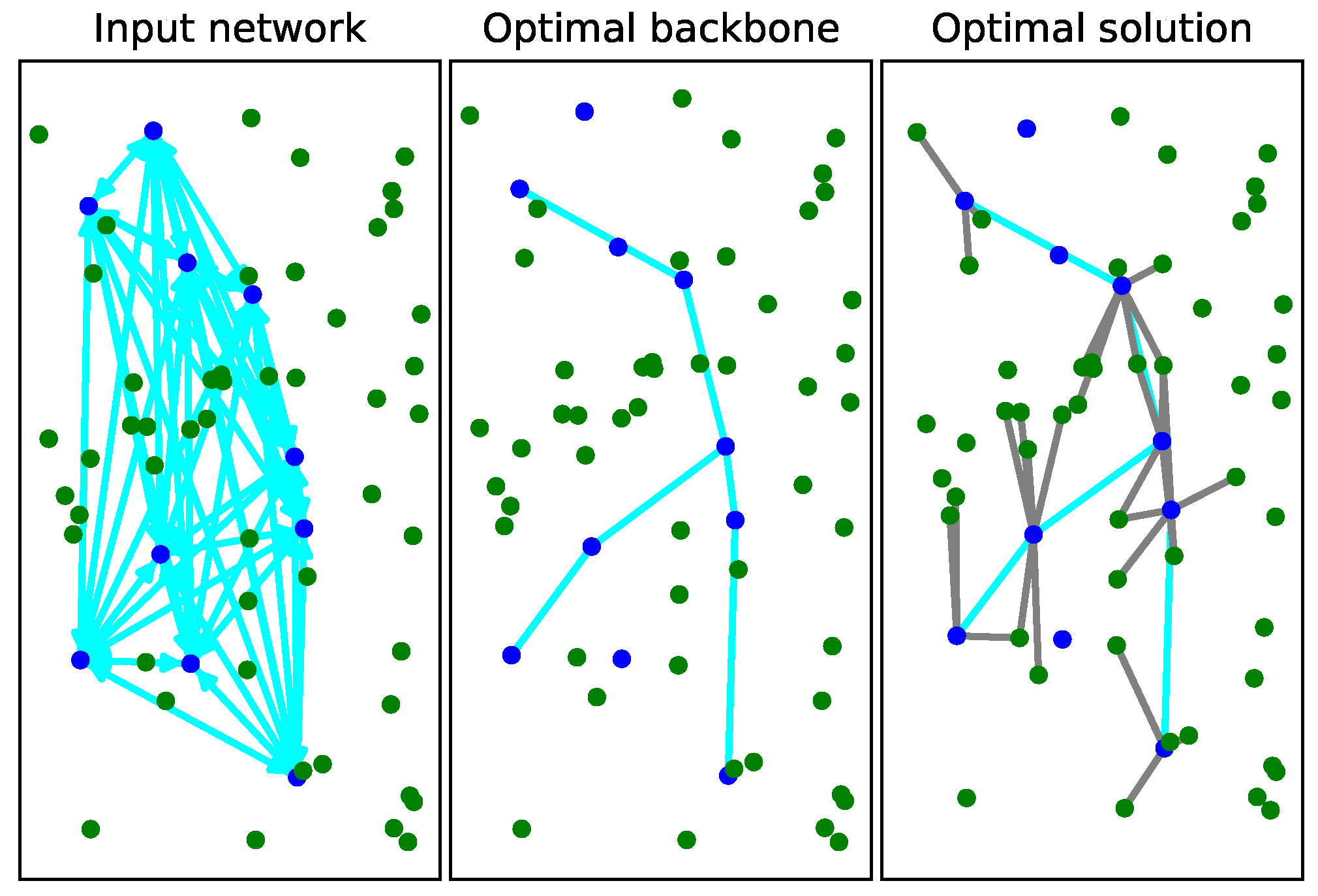
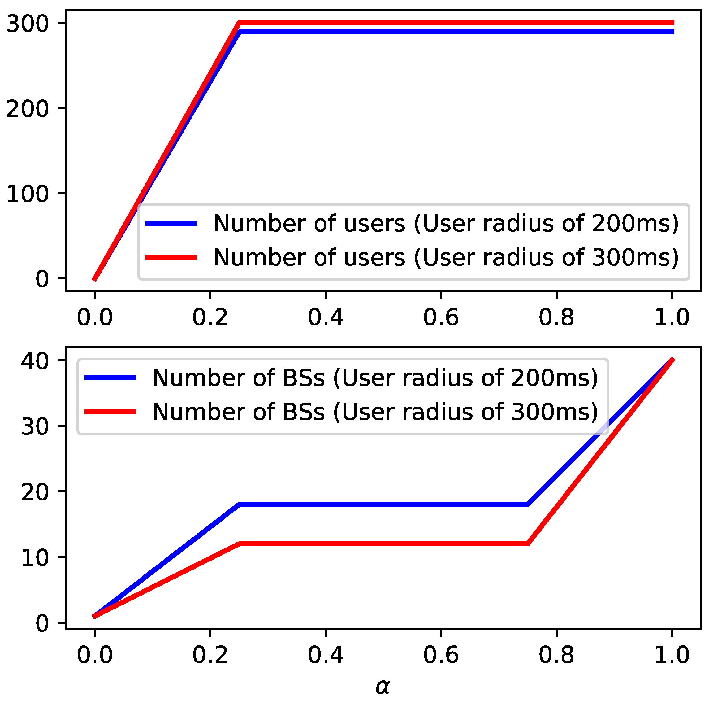
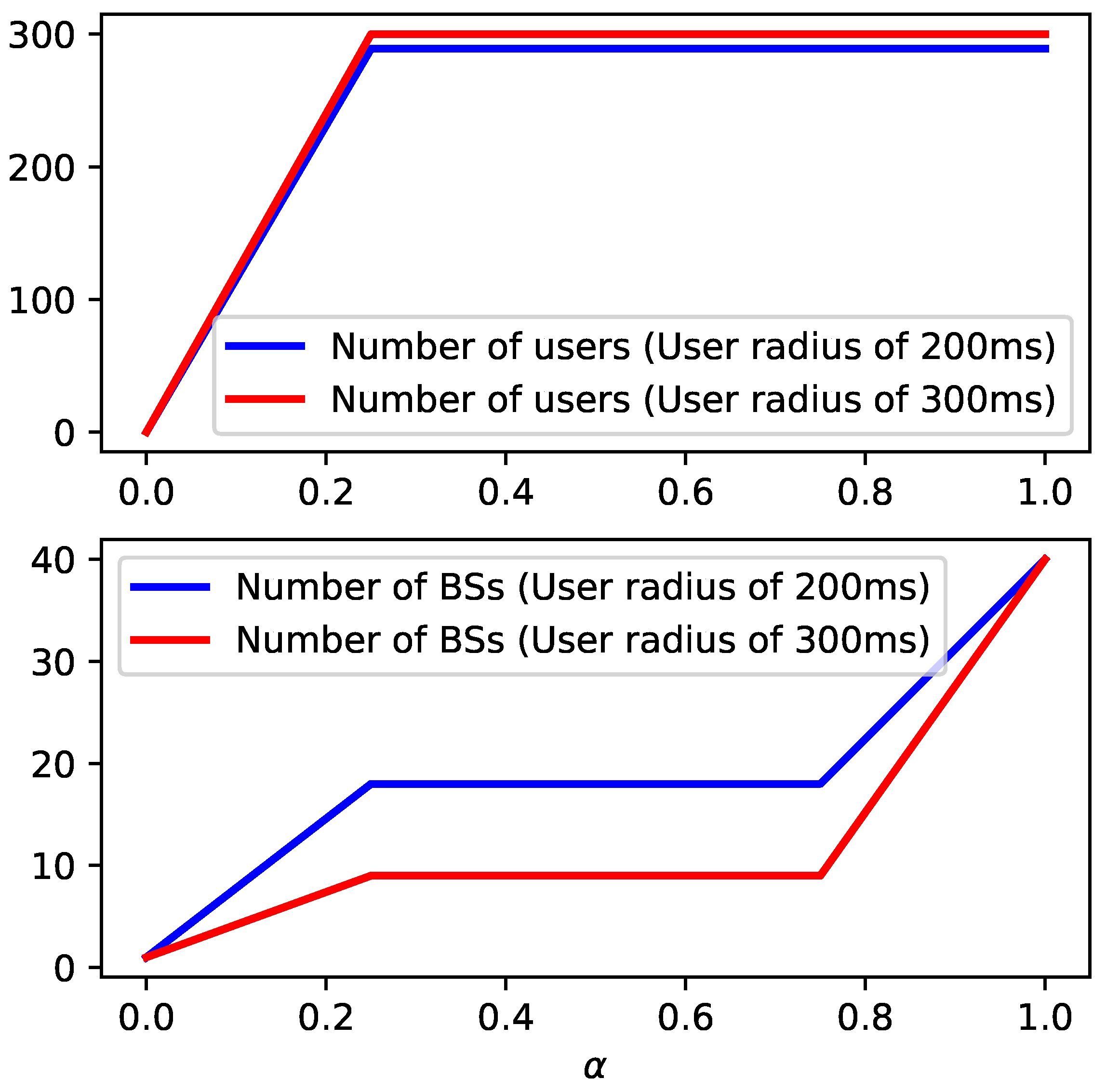
To give more insights concerning the behavior of model M 1 , in Figure 3 and Figure 4 the impact of varying parameter α [ 0 ; 1 ] for a sparse and a complete input graph, respectively, is plotted. For both figures, the number of covered users and active BSs is plotted while also varying the transmission radius between BSs and users from 200 ms to 300 ms. Each instance is composed of n = 40 BSs and m = 300 users. We mention that each point in these curves corresponds to an optimal solution to the problem.
From Figure 3 and Figure 4, one can see that the higher the transmission radius between BSs and users is, the higher the number of covered users. Additionally, the lower the number of BSs required to connect the backbone network. In particular, in Figure 4, the number of active BSs is less than in Figure 3 since the backbone is fully connected. Finally, it is observed that the objective values increase with parameter α . In Table 5 and Table 6, the numerical results obtained with Algorithm 2 for the sparse and complete graph instances, respectively, solved in the previous tables are reported. In particular, in Table 5 and Table 6, the same column information is reported. More precisely, in columns 1–3, the instance number, the density of the graph, and the value of parameter α are reported. Next, in columns 4–10, the best objective value obtained in the previous tables, the best objective found with Algorithm 1, the CPU time in seconds required by the algorithm, its number of iterations, the number of attended or covered users in the network instance, and the number of BSs required to connect the backbone in the output solution of the problem are reported. Finally, the gaps in percentage that we compute by t h e   v a l u e   o f   c o l u m n   4     t h e   v a l u e   o f   c o l u m n   5 t h e   v a l u e   o f   c o l u m n   4 100 are reported. From these tables, one can observe that the solutions obtained by the proposed local search heuristic are near-optimal, with a worst gap obtained of 0.88% in the case of the sparse graphs and a worst gap of 3.03% for the complete graphs. It is further noted that the worst CPU time is lower than one minute for all the tested instances. One can also see that the larger the value of parameter α , the larger the number of BSs required to construct the backbone. Finally, it is observed that most of the users are covered for all tested instances. To further investigate the behavior of Algorithm 2, in Table 7 and Table 8 numerical results obtained with M 1 versus Algorithm 2 for a large sparse connected and a fully connected graph instance, respectively, are compared. In these tables, the legend is the same. In columns 1–3, the instance number, the density of the graph, and the value of the parameter α are reported. Next, in columns 4–6, the best objective function value of model M 1 , the number of branch and bound nodes, and its CPU time in seconds are presented. Subsequently, the best objective value obtained with Algorithm 2, its CPU time in seconds, the number of iterations of the algorithm, the number of covered users, the number of active BSs, and the gaps in percentage that we compute by t h e   v a l u e   o f   c o l u m n   4     t h e   v a l u e   o f   c o l u m n   7 t h e   v a l u e   o f   c o l u m n   4 100 are shown. From Table 7 and Table 8, it is observed that M 1 requires more than one hour to obtain the optimal solution except for the instances using α = 1 . In this case, the problem becomes much more simple to solve optimally. Next, one can observe that the Algorithm 2 has an even better performance with a worst gap percentage of 0.21%. Finally, one can also see that most of the users are covered without using a large number of active BSs forming the backbone.
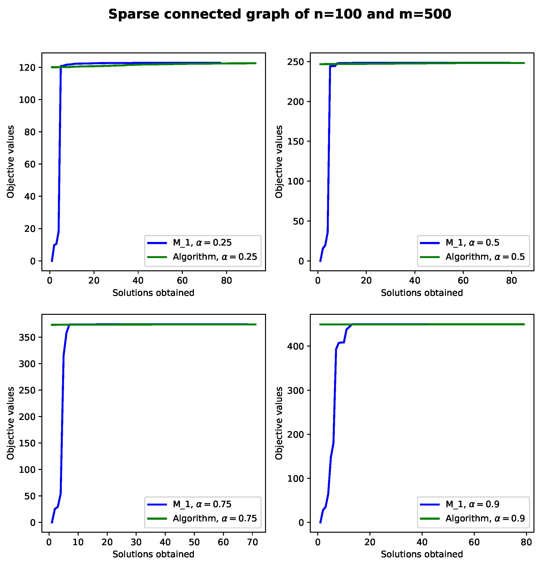
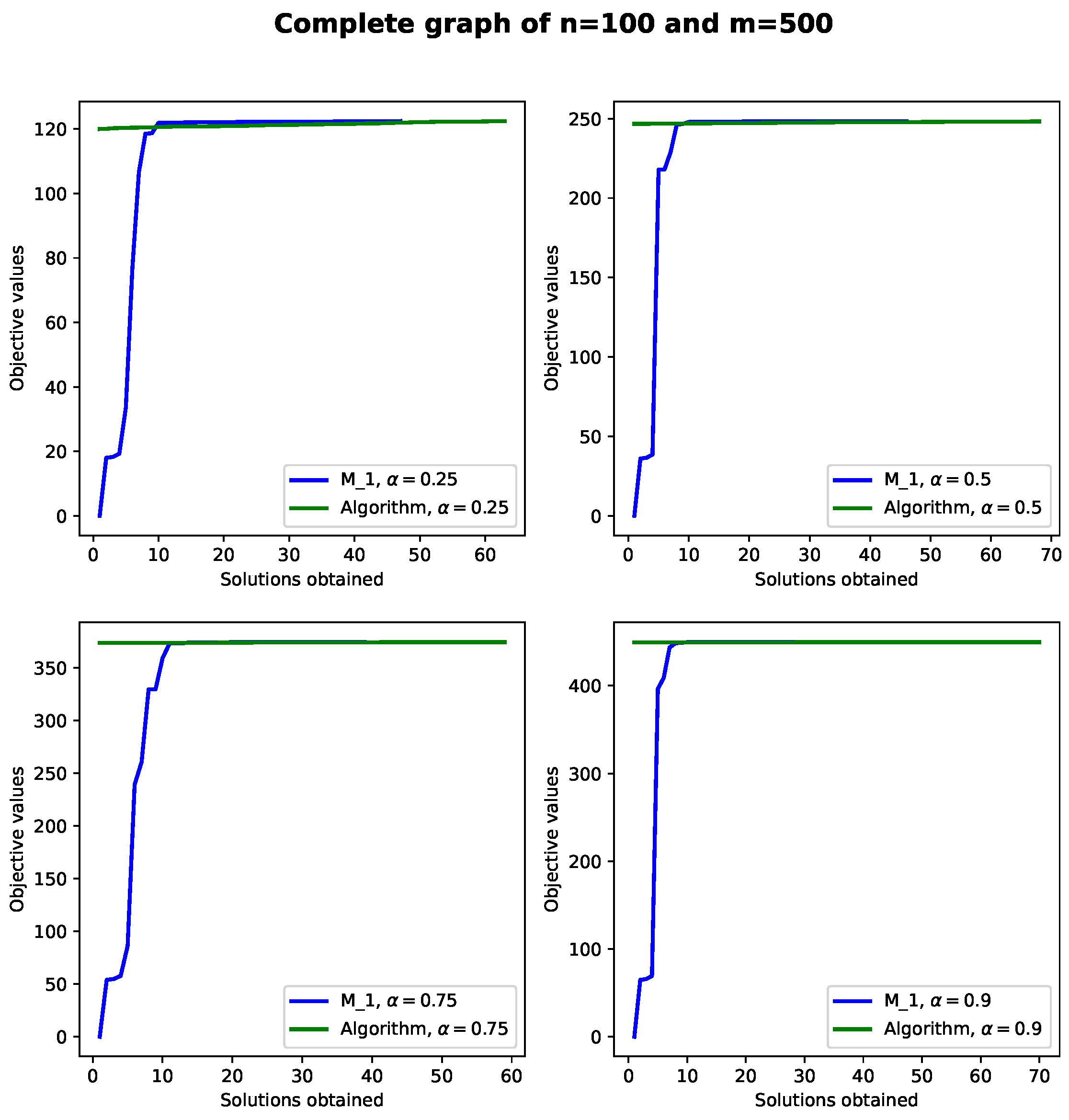
To provide further insights concerning the behavior of Algorithm 2, in Figure 5 and Figure 6 feasible solutions in terms of objective values for a sparsely and fully connected input network obtained with M 1 while varying α in the interval [0.25;0.9] are presented. In both figures, each network is composed of n = 100 nodes for the backbone and m = 500 users. In particular, in Figure 5 a radial transmission distance of 300 ms for the BSs is used and 200 ms for the distances between BSs and users. In Figure 6, the distances between BSs and users are set to 200 ms as well. Finally, we mention that both figures report objective values and velocities obtained with M 1 and Algorithm 2 when finding feasible solutions. The numerical results obtained in Figure 5 and Figure 6 show that CPLEX finds very poor solutions at the beginning. More precisely, CPLEX takes at least 10 s to reach good quality solutions, whereas Algorithm 2 can find very good objective values in fractions of a second. After this time, it is observed that CPLEX and Algorithm 2 are both competitive in the sense that they reach similar solutions. Another observation is that one can ensure that the objective values are near-optimal ones. This can be ensured because the Mipgaps obtained with CPLEX are lower than 1% [7]. Finally, it is observed that varying the parameter α does not seem to have a significant effect on the performance of either M 1 or the Algorithm 2. However, note that the higher the value of the parameter α , the larger the number of users that can be covered.

6. Conclusions

This article considers the problem of how to connect nodes in a network while covering as many users as possible at a minimum connectivity cost simultaneously for 5G networks. It is well known that 5G technology is fast, but it is a bit tricky because it does not cover long distances well when using millimeter-wave technology. Consequently, we proposed new mathematical formulations to solve this problem from a management point of view. These models help us decide which nodes in the network should be connected to cover most of the users. Our models are solved with the branch and cut and Benders decomposition algorithms of the CPLEX solver to find the optimal solutions. We also proposed an exact iterative approach to solve the exponential model and proposed an approximation meta-heuristic algorithm to find good solutions faster. In our tests, we found that solving the problem perfectly is hard. We could only do it for cases with up to 40 nodes and 500 users. One of our models worked better in terms of time. On the other hand, our meta-heuristic showed that we could obtain tight solutions with less effort for both small and large graph instances using symmetric radial transmission distances. Finally, we mention that since our proposed exponential model is solved iteratively with our exact approach, we could obtain tight upper bounds. On the other hand, since the rest of the models obtain in the best case the optimal or feasible lower bounds, we provided a tight interval while ensuring that the optimal solutions lie inside that interval. Ultimately, since there are no models proposed in the literature covering both aspects at the same time, there are no benchmark instances to compare with yet in the literature. Thus, we believe that these models will enrich the literature to develop further modeling aspects of the problem and will allow for benchmark comparisons.
In future research, new avenues to be considered for the network planning problem are suggested as follows. First, we mention that the proposed models can include nonlinear formulas such as capacity and interference which can potentially lead to more difficult formulations to deal with. Furthermore, if the arising nonlinearities are nonconvex, there would be no certification of optimality. Thus, this constitutes a challenging task to perform in future research. Finally, another research direction is to consider exploring urban areas, even though this would require realistic data from particular cities while also considering non-line-of-sight aspects when using symmetric and asymmetric radial transmission distance costs as well as new mathematical models and algorithms to solve this relevant network planning problem from a management point of view.

Author Contributions

Conceptualization, P.A., A.D.F. and S.C.; methodology, P.A., A.D.F. and S.C.; software, P.A., A.D.F. and S.C.; validation, P.A. and A.D.F.; formal analysis, P.A., A.D.F. and S.C.; investigation, P.A., A.D.F. and S.C.; resources, P.A. and A.D.F.; data curation, P.A., A.D.F. and S.C.; writing—original draft preparation, P.A., A.D.F. and S.C.; writing—review and editing, P.A. and A.D.F.; visualization, P.A., A.D.F. and S.C.; supervision, P.A.; project administration, P.A. and A.D.F.; funding acquisition, P.A. and A.D.F. All authors have read and agreed to the published version of the manuscript.

Funding

The authors acknowledge the financial support from Projects Dicyt 062313AS, ANID/FONDECYT Iniciación No. 11230129, and the Competition for Research Regular Projects, year 2021, code LPR21-02; Universidad Tecnológica Metropolitana.

Data Availability Statement

Dataset available on request from the authors.: The raw data supporting the conclusions of this article will be made available by the authors on request.

Acknowledgments

The authors acknowledge the support of the Vicerrectoría de Investigación, Innovación y Creación (VRIIC) of the Universidad de Santiago de Chile.

Conflicts of Interest

The authors declare no conflicts of interest.

References

  1. IEEE 5G and Beyond Technology Road Map. 2020. Available online: https://futurenetworks.ieee.org/images/files/pdf/ieee-5g-roadmap-white-paper.pdf (accessed on 30 May 2023).
  2. Palizban, N. Millimeter Wave Small Cell Network Planning for Outdoor Line-of-Sight Coverage Millimeter Wave Small Cell Network Planning for Outdoor. Ph.D. Thesis, Carleton University, Ottawa, ON, Canada, 2017. [Google Scholar]
  3. Rappaport, T.S.; Sun, S.; Mayzus, R.; Zhao, H.; Azar, Y.; Wang, K.; Wong, G.N.; Schulz, J.K.; Samimi, M.; Gutierrez, F. Millimeter wave mobile communications for 5G cellular: It will work! IEEE Access 2013, 1, 335–349. [Google Scholar] [CrossRef]
  4. Rakuten, Reimagining the End-to-End Mobile Network in the 5G Era. 2019. Available online: https://www.cisco.com/c/dam/en/us/products/collateral/cloud-systems-management/elastic-services-controller-esc/reimagining-mobile-network-white-paper.pdf (accessed on 30 May 2023).
  5. Niu, Y.; Li, Y.; Jin, D.; Su, L.; Vasilakos, A.V. A survey of millimeter wave communications (mmWave) for 5G: Opportunities and challenges. Wirel. Netw. 2015, 21, 2657–2676. [Google Scholar] [CrossRef]
  6. Adasme, P. p-Median based formulations with backbone facility locations. Appl. Soft Comput. 2018, 67, 261–275. [Google Scholar] [CrossRef]
  7. IBM ILOG, CPLEX High-Performance Mathematical Programming Engine, V20.1.0, (2020). Available online: http://www.ibm.com/software/integration/optimization/cplex/ (accessed on 10 June 2023).
  8. Rahmaniani, R.; Crainic, T.G.; Gendreau, M.; Rei, W. The Benders decomposition algorithm: A literature review. Eur. J. Oper. Res. 2017, 259, 801–817. [Google Scholar] [CrossRef]
  9. Adasme, P.; Cordero, S.; Soto, I.; Firoozabadi, A.D. New Formulations for Optimal User Coverage using 5G Millimeter-Wave-based Networks. In Proceedings of the 2022 13th International Symposium on Communication Systems, Networks and Digital Signal Processing (CSNDSP), Porto, Portugal, 20–22 July 2022; pp. 732–737. [Google Scholar]
  10. Rezaei, A.; Mascheroni, A.; Stevens, M.C.; Argha, R.; Papandrea, M.; Puiatti, A.; Lovell, N.H. Unobtrusive Human Fall Detection System Using mmWave Radar and Data Driven Methods. IEEE Sensors J. 2023, 23, 7968–7976. [Google Scholar] [CrossRef]
  11. Anjinappa, C.K.; Erden, F.; Güvenç, I. Base Station and Passive Reflectors Placement for Urban mmWave Networks. IEEE Trans. Veh. Technol. 2021, 70, 3525–3539. [Google Scholar] [CrossRef]
  12. Gu, Z.; Lu, H.; Zhang, M.; Sun, H.; Chen, C.W. Association and Caching in Relay-Assisted mmWave Networks: A Stochastic Geometry Perspective. IEEE Trans. Wirel. Commun. 2021, 12, 8316–8332. [Google Scholar] [CrossRef]
  13. Szyszkowicz, S.S.; Lou, A.; Yanikomeroglu, H. Automated Placement of Individual Millimeter-Wave Wall-Mounted Base Stations for Line-of-Sight Coverage of Outdoor Urban Areas. IEEE Wirel. Commun. Lett. 2016, 5, 316–319. [Google Scholar] [CrossRef]
  14. Sandoval, C.; Adasme, P.; Juan, E.S.; Soto, I.; Firoozabadi, A.D. Novel p-Median-based Formulations for Maximizing Coverage in 5G/6G Wireless Networks. In Proceedings of the 2021 Third South American Colloquium on Visible Light Communications (SACVLC), Toledo, Brazil, 11–12 November 2021; pp. 1–5. [Google Scholar] [CrossRef]
  15. Koutsaftis, A.; Kumar, R.; Liu, P.; Panwar, S.S. Fast Inter-Base Station Ring (FIBR): A New Millimeter Wave Cellular Network Architecture. IEEE J. Sel. Areas Commun. 2019, 37, 2699–2714. [Google Scholar] [CrossRef]
  16. Sabzehali, J.; Shah, V.K.; Dhillon, H.S.; Reed, J.H. 3D Placement and Orientation of mmWave-Based UAVs for Guaranteed LoS Coverage. IEEE Wirel. Commun. Lett. 2021, 10, 1662–1666. [Google Scholar] [CrossRef]
  17. Fortet, R. Applications de lálgebre de boole en recherche operationelle. Rev. Fr. Rech. Oper. 1960, 4, 17–26. [Google Scholar]
  18. Letchford, A.N.; Nasiri, S.D. Dirk Oliver Theis: Compact formulations of the Steiner Traveling Salesman Problem and related problems. Eur. J. Oper. Res. 2013, 228, 83–92. [Google Scholar] [CrossRef]
  19. Adasme, P.; Andrade, R.; Letournel, M.; Lisser, A. Stochastic maximum weight forest problem. Networks 2015, 65, 289–305. [Google Scholar] [CrossRef]
  20. Cormen, T.H.; Leiserson, C.E.; Rivest, R.L.; Stein, C. Introduction to Algorithms; MIT Press and McGraw-Hill: Cumberland, RI, USA, 2009. [Google Scholar]
Figure 1. Input network, the optimal backbone solution of a sparse graph, and the users connected to the active BSs. The solution is obtained using α = 0.5 for m = 50 users. The network is composed of n = 10 nodes using radial transmission distances of 300 ms between BSs. The radial transmission distance between users and BSs is 200 ms. BSs are colored blue and users are colored green.
Symmetry 16 00123 g001
Figure 2. Input network, the optimal backbone solution of a complete graph. The solution is obtained using α = 0.5 for m = 50 users. The network is composed of n = 10 nodes. The radial transmission distance between users and BSs is 200 ms. BSs are colored blue and users are colored green.
Symmetry 16 00123 g002
Figure 3. Impact of varying parameter α [ 0 ; 1 ] for a sparse input graph with transmission radius between BSs of 300 m, and transmission radii between BSs and users of 200 m and 300 m. The instance is composed of n = 40 BSs and 300 users.
Symmetry 16 00123 g003
Figure 4. Impact of varying parameter α [ 0 ; 1 ] for a complete input graph using transmission radii between BSs and users of 200 m and 300 m. The instance is composed of n = 40 BSs and 300 users.
Symmetry 16 00123 g004
Figure 5. Feasible solutions obtained with M 1 and Algorithm 2 for a sparse connected input network while varying α in the interval [ 0.25 ; 0.9 ] .
Symmetry 16 00123 g005
Figure 6. Feasible solutions obtained with M 1 and Algorithm 2 for a fully connected input network while varying α in the interval [ 0.25 ; 0.9 ] .
Symmetry 16 00123 g006
Table 1. Numerical results obtained with M 1 and M 2 for sparse connected graphs.
#Density α M 1 (B&C) M 1 (Benders) M 2 (B&C) M 2 (Benders)
Best B & Bn CPU (s)Best B & Bn CPU (s)Best B & Bn CPU (s)Best B & Bn CPU (s)
Using n = 40 , m = 250 , a radius of 200 m for users, and a radius of 300 m for BSs
123.580.2559.4558,84395.3759.45155,65750.1459.45919,3533600.0959.4572,49932.81
20.5121.9636,49763.01121.9680,22523.32121.96623,8923600.07121.9685,50722.06
30.75184.4815,51622.13184.4873843.25184.48633,2563600.23184.48123,394104.57
41247.000.12247.09600.37247.000.34247.000.26
Using n = 40 , m = 500 , a radius of 200 m for users, and a radius of 300 m for BSs
520.120.25121.6427,37535.82121.64150,20379.89121.641,103,8033600.06121.6466,04231.03
60.5246.43781512.07246.4316,2567.56246.43909,9623600.07246.43136,10178.51
70.75371.2131654.18371.2113,6767.18371.211,290,4873600.06371.2115,60712.1
81496.000.09496.010830.46496.001.25496.000.32
Using n = 60 , m = 250 , a radius of 200 m for users, and a radius of 300 m for BSs
921.410.2559.63256,1953600.0659.47374,1243602.3759.5697,9533600.259.52452,2933601.43
100.5122.42113,3473600.07122.37439,4333600.92122.3944,6283601.76121.93113,6983604.0
110.75185.21228,7173600.42185.14197,1593600.54185.1738,2093606.07185.0188,1913601.43
121248.003.1248.0329278.78248.001.71248.001.71
Using n = 60 , m = 500 , a radius of 200 m for users, and a radius of 300 m for BSs
1321.580.25116.32345,3803600.04116.27374,3713600.11116.3275,1103604.03115.81173,9443628.18
140.5235.55196,1243600.21235.56869,0843602.04235.5546,3423609.23235.5111,9893604.75
150.75354.77496,4383600.43354.77545,8243604.79354.7650,4193602.45354.0619,1103601.76
161474.004.29474.0254755.48474.001.43474.001.78
Table 2. Numerical results obtained with M 1 and M 2 for complete connected graphs.
#Density α M 1 (B&C) M 1 (Benders) M 2 (B&C) M 2 (Benders)
Best B & Bn CPU (s)Best B & Bn CPU (s)Best B & Bn CPU (s)Best B & Bn CPU (s)
Using n = 40 , m = 250 , and a radius of 200 m for users
11000.2559.515,16280.7559.537,82822.1159.5200,7783606.4259.5100,908684.62
20.5122.012,08882.32122.021,70714.67121.98178,1753600.64122.0251,3622044.93
30.75184.523,701142.43184.5747212.25184.5330,2503600.21184.525,61953.4
41247.000.32247.000.07247.000.23247.000.31
Using n = 40 , m = 500 , and a radius of 200 m for users
51000.25121.0618,23979.29121.0630254.53121.06232,4443603.07121.06103,0161118.95
60.5245.37450433.35245.3730702.93245.37244,2233600.89245.3745,515432.28
70.75369.68850829.0369.6711172.14369.68494,0943603.0369.68646893.06
81494.000.21494.000.07494.002.71494.000.35
Using n = 60 , m = 250 , and a radius of 200 m for users
91000.2559.6373,3323600.0759.21642,6113600.159.5449,0673609.057.5732883601.4
100.5122.4108,2143600.15121.761,061,0653601.32122.2913,4403602.01120.3124443601.96
110.75185.297,0163603.7185.03209,4603600.76185.1814,8943604.04184.5314133603.48
121248.004.59248.000.28248.001.03248.001.23
Using n = 60 , m = 500 , and a radius of 200 m for users
131000.25116.3285,3823601.98116.25338,2783600.78116.3318,5213602.010.003600.4
140.5235.5560,5373600.95235.53469,5643601.87235.5223,2593608.820.003600.17
150.75354.7775,3853601.1354.77348,2523602.75354.7774,4683609.10.003600.48
161474.008.53474.002.7474.007.7474.001.2
Table 3. Numerical results obtained with M 3 and M 4 for sparse connected graphs.
#Density α M 3 (B&C) M 3 (Benders) M 4
Best B & Bn CPU (s)Best B & Bn CPU (s)BestCPU (s)Iter.Gap
Using n = 40 , m = 250 , a radius of 200 m for users, and a radius of 300 m for BSs
123.580.2559.457,053,0833601.2159.454,436,0103607.1759.53622.523120.09
20.5121.963,277,4303600.54121.963,876,7203600.32122.03609.393540.03
30.75184.482,246,2983600.43184.482,568,6633600.39184.493604.514560.0
41247.0122.0247.0222.06247.00.65320.0
Using n = 40 , m = 500 , a radius of 200 m for users, and a radius of 300 m for BSs
520.120.25121.642,310,2193600.7121.635,923,0553601.34121.773688.812490.1
60.5246.435,124,8413601.42246.424,388,9093602.64246.53675.532830.02
70.75371.213,810,3063600.42371.23,881,5113600.46371.243656.923760.0
81496.001.89496.01684.4496.00.51210.0
Using n = 60 , m = 250 , a radius of 200 m for users, and a radius of 300 m for BSs
921.410.2559.612,739,8003679.9259.51,469,4573647.2559.963740.32735.92
100.5122.411,374,9753621.26122.332,021,2883608.48122.643712.91760.18
110.75185.22,851,1453702.12185.181,550,6393669.54185.323654.23750.06
121248.008.56248.01577.76248.01.28320.0
Using n = 60 , m = 500 , a radius of 200 m for users, and a radius of 300 m for BSs
1321.580.25116.342,518,4693681.64116.286,596,1253605.45116.623669.21020.24
140.5235.553,802,3303607.9235.523,095,7303614.51235.743763.581070.08
150.75354.773,260,8363604.92354.744,077,0343601.5354.873627.481290.02
161474.001.21474.01532.76474.00.3750.0
Table 4. Numerical results obtained with M 3 and M 4 for complete graphs.
#Density α M 3 (B&C) M 3 (Benders) M 4
Best B & Bn CPU (s)Best B & Bn CPU (s)BestCPU (s)Iter.Gap
Using n = 40 , m = 250 , and a radius of 200 m for users
11000.2559.53,387,8732498.8459.56,118,7033600.1759.513632.322540.02
20.5122.01,913,2083600.31122.03,007,1313600.39122.03620.282700.0
30.75184.51,681,0663600.42184.492,235,4753600.54184.53281.323200.0
41247.001.4247.000.32247.00.220.0
Using n = 40 , m = 500 , and a radius of 200 m for users
51000.25121.054,596,5833601.4121.053,106,3273603.67121.183625.982250.1
60.5245.371,743,0753600.42245.361,871,5853600.56245.443618.882590.03
70.75369.681,013,6763600.56369.684,572,2593604.63369.73616.543740.0
81494.000.5494.000.17494.00.3920.0
Using n = 60 , m = 250 , and a radius of 200 m for users
91000.2559.61567,3163602.459.59506,3173601.0159.973621.19560.61
100.5122.42308,9863600.93122.36544,4333605.35122.643646.03580.18
110.75185.2151,1273601.96185.17269,6323602.04185.323610.28690.06
121248.000.4248.000.21248.00.8520.0
Using n = 60 , m = 500 , and a radius of 200 m for users
131000.25116.33463,9613605.71116.25329,2603602.73116.633661.73900.26
140.5235.55183,0343601.18235.52531,1163603.63235.753627.84930.08
150.75354.77134,8543601.84354.73275,6133602.2354.873620.451140.02
161474.000.6474.000.28474.00.520.0
Table 5. Numerical results obtained with Algorithm 2 for sparse connected graphs.
#Density α Algorithm 2
BestBest Alg.CPU (s) Alg.# Iter.# of Users# of BSsGap (%)
Using n = 40 , m = 250 , a radius of 200 m for users, and a radius of 300 m for BSs
123.580.2559.4559.193.893258247230.42
20.5121.96121.794.033494247240.13
30.75184.48184.378.557059247240.05
41247.0246.08.292700246390.4
Using n = 40 , m = 500 , a radius of 200 m for users, and a radius of 300 m for BSs
520.120.25121.64120.568.545271493280.88
60.5246.43245.2412.137172494290.47
70.75371.21368.8916.0911,781493270.62
81496.0492.09.352672492400.8
Using n = 60 , m = 250 , a radius of 200 m for users, and a radius of 300 m for BSs
921.410.2559.6359.385.515411248240.4
100.5122.42122.218.216970248260.16
110.75185.21185.1310.268294248240.04
121248.0248.015.322501248600.0
Using n = 60 , m = 500 , a radius of 200 m for users, and a radius of 300 m for BSs
1321.580.25116.32115.9125.1612,553473240.35
140.5235.55235.4423.2411,981474240.04
150.75354.77353.2220.047988472230.43
161474.0471.018.572519471580.63
Table 6. Numerical results obtained with Algorithm 2 for complete graphs.
#Density α Algorithm 2
BestBest Alg.CPU (s) Alg.# Iter.# of Users# of BSsGap (%)
Using n = 40 , m = 250 , and a radius of 200 m for users
11000.2559.559.227.0510,151247240.49
20.5122.0121.7923.738555247260.16
30.75184.5183.6420.247353246260.46
41247.0246.019.894246246370.4
Using n = 40 , m = 500 , and a radius of 200 m for users
51000.25121.06118.2226.246389484282.33
60.5245.37241.1553.3712,623486281.71
70.75369.68363.5941.869742486271.64
81494.0479.031.125317479393.03
Using n = 60 , m = 250 , and a radius of 200 m for users
91000.2559.6359.3419.646439248260.48
100.5122.4122.2222.218635248250.14
110.75185.2185.0914.284935248260.05
121248.0248.026.082501248600.0
Using n = 60 , m = 500 , and a radius of 200 m for users
131000.25116.32115.9232.098958473250.34
140.5235.55234.9222.895601473270.26
150.75354.77353.9936.449848473250.21
161474.0471.032.092692471600.63
Table 7. Numerical results obtained with M 1 vs. Algorithm 2 for a large sparse connected graph instance.
#Density α M 1 Algorithm 2
Best B & Bn CPU (s)Best Alg.CPU (s) Alg.# Iter.# of Users# of BSsGap (%)
Using n = 100 , m = 1000 , a radius of 200 ms between users and BSs, and a radius of 300 ms between BSs
122.820.25247.62133,5803603.95247.1265.8411,0701000370.19
20.5498.45140,3503603.35498.0955.5799781000360.07
30.75749.2129,1263600.81749.0338.173271000380.02
411000.001.28999.048.472504999970.1
Table 8. Numerical results obtained with M 1 vs. Algorithm 2 for a complete graph instance.
#Den. α M 1 Algorithm 2
Best B & Bn CPU (s)Best Alg.CPU (s) Alg.# Iter.# of Users# of BSsGap (%)
Using n = 100 , m = 1000 , a radius of 200 ms between users and BSs, and a radius of 300 ms between BSs
11000.25247.5813,6973600.23247.0552.8463381000360.21
20.5498.3882973600.26498.1577.9910,6101000320.04
30.75749.2197923600.18749.0692.7411,8631000350.01
411000.003.82999.081.892507999970.1
Disclaimer/Publisher’s Note: The statements, opinions and data contained in all publications are solely those of the individual author(s) and contributor(s) and not of MDPI and/or the editor(s). MDPI and/or the editor(s) disclaim responsibility for any injury to people or property resulting from any ideas, methods, instructions or products referred to in the content.

