
Implementing a Relativistic Motor over Atomic Scales


Abstract
:1. Introduction
- Allows three-axis motion (including vertical);
- No moving parts;
- Zero fuel consumption;
- Zero carbon emission;
- Needs only electromagnetic energy (which may be provided by solar panels);
- Highly efficient, in principle, kinetic energy can be converted back to electromagnetic energy.
2. Relativistic Engine in the Microscopic Scale
2.1. A Classical Electron
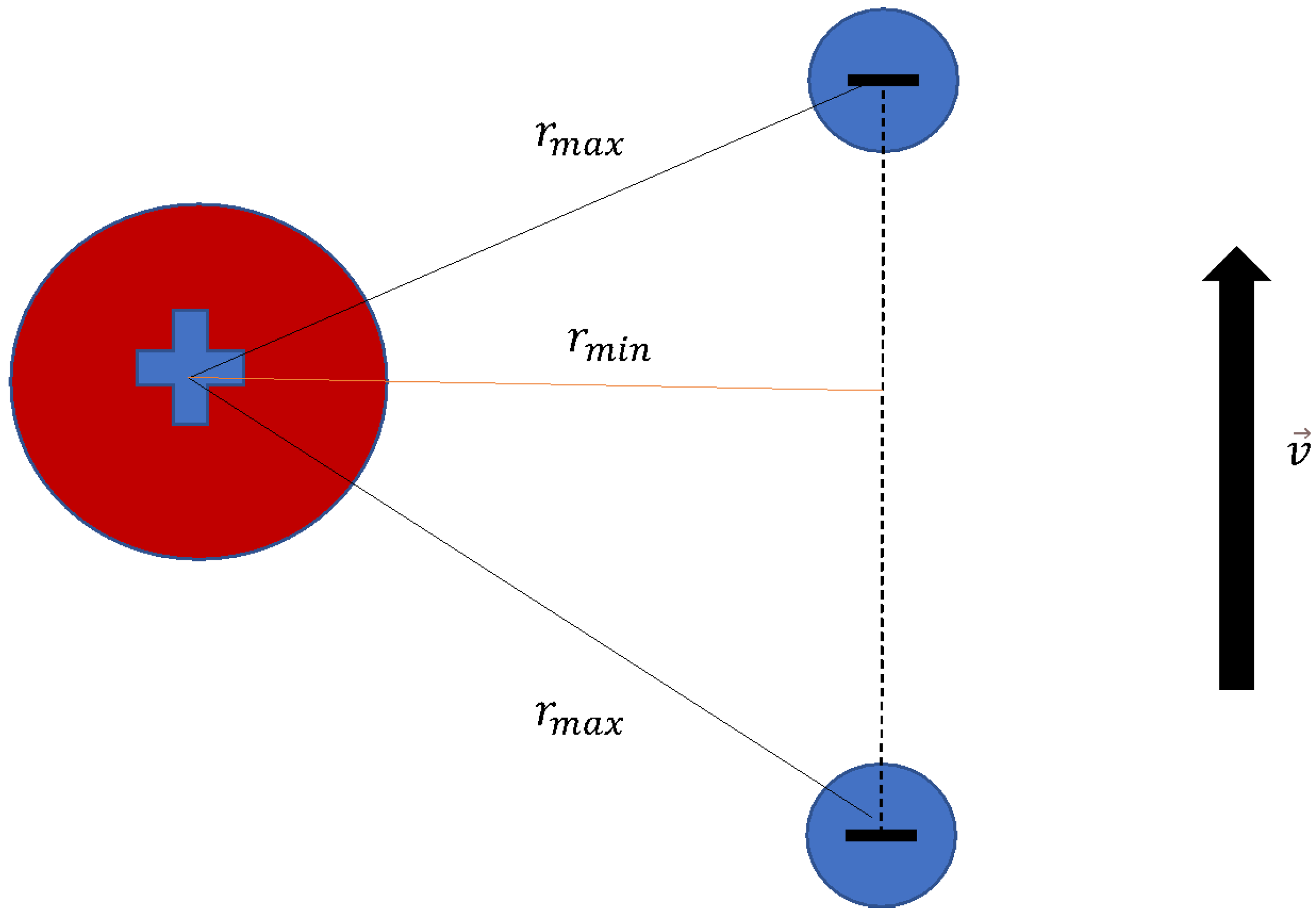
2.1.1. Proximity Considerations
2.1.2. An Unconfined Electron
2.1.3. A Confined Electron
3. Schrödinger’s Electron
4. Pauli’s Electron
5. The Hydrogen Atom
6. A Simple Wave Packet
7. Discussion
8. Conclusions
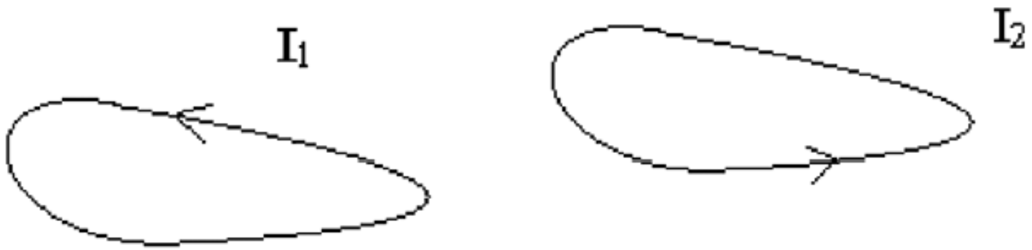
- Analysis of a relativistic engine with components that move at relativistic speeds (and not just the electromagnetic signals transmitted between the components). The need for this arises as the electron studied in the current paper is relativistic.
- A study of the relativistic motor in the framework of a Dirac theory is required. The Schrödinger equation and the Pauli equation are not sufficient for the study of an electron at relativistic speeds.
Funding
Data Availability Statement
Conflicts of Interest
References
- Tuval, M.; Yahalom, A. Momentum Conservation in a Relativistic Engine. Eur. Phys. J. Plus 2016, 131, 374. [Google Scholar] [CrossRef]
- Feynman, R.P.; Leighton, R.B.; Sands, M.L. Feynman Lectures on Physics, 50th ed.; Basic Books: New York, NY, USA, 2011. [Google Scholar]
- Jackson, J.D. Classical Electrodynamics, 3rd ed.; Wiley: New York, NY, USA, 1999. [Google Scholar]
- Yahalom, A. Newton’s Third Law in the Framework of Special Relativity for Charged Bodies Part 2: Preliminary Analysis of a Nano Relativistic Motor. Symmetry 2022, 14, 94. [Google Scholar] [CrossRef]
- Tuval, M.; Yahalom, A. Newton’s Third Law in the Framework of Special Relativity. Eur. Phys. J. Plus 2014, 129, 240. [Google Scholar] [CrossRef]
- Griffiths, D.J.; Heald, M.A. Time dependent generalizations of the Biot-Savart and Coulomb laws. Am. J. Phys. 1991, 59, 111–117. [Google Scholar] [CrossRef]
- Jefimenko, O.D. Electricity and Magnetism, 2nd ed.; Electret Scientific: Star City, WV, USA, 1989. [Google Scholar]
- Yahalom, A. Retardation in Special Relativity and the Design of a Relativistic Motor. Acta Phys. Pol. A Vol. 2017, 131, 1285–1288. [Google Scholar] [CrossRef]
- Mansuripur, M. Trouble with the Lorentz Law of Force: Incompatibility with Special Relativity and Momentum Conservation. PRL 2012, 108, 193901. [Google Scholar] [CrossRef] [PubMed]
- Rajput, S.; Yahalom, A.; Qin, H. Lorentz Symmetry Group, Retardation and Energy Transformations in a Relativistic Engine. Symmetry 2021, 13, 420. [Google Scholar] [CrossRef]
- Shailendra, R.; Yahalom, A. Newton’s Third Law in the Framework of Special Relativity for Charged Bodies. Symmetry 2021, 13, 1250. [Google Scholar] [CrossRef]
- Dielectric Strength of Air—The Physics Fact Book. Available online: https://hypertextbook.com/facts/2000/AliceHong.shtml (accessed on 20 August 2023).
- Giere, S.; Kurrat, M.; Schumann, U. HV Dielectric Strength of Shielding Electrodes in Vacuum Circuit-Breakers. In Proceedings of the 20th International Symposium on Discharges and Electrical Insulation in Vacuum, Tours, France, 1–5 July 2002. [Google Scholar]
- Volpe, P.-N.; Muret, P.; Pernot, J.; Omnès, F.; Teraji, T.; Jomard, F.; Planson, D.; Brosselard, P.; Dheilly, N.; Vergne, B.; et al. High breakdown voltage Schottky diodes synthesized on p-type CVD diamond layer. Phys. Status Solidi A 2010, 207, 2088–2092. Available online: https://onlinelibrary.wiley.com/doi/abs/10.1002/pssa.201000055 (accessed on 10 August 2013). [CrossRef]
- Lo, H.W.; Tai, Y.C. Parylene-based electret power generators. J. Micromech. Microeng. 2008, 18, 104006. [Google Scholar] [CrossRef]
- Jung, S.-G.; Kang, J.-H.; Park, E.; Lee, S.; Lin, J.-Y.; Chareev, D.A.; Vasiliev, A.N.; Park, T. Enhanced critical current density in the pressure-induced magnetic state of the high-temperature superconductor FeSe. Sci. Rep. 2015, 5, 16385. [Google Scholar] [CrossRef] [PubMed]
- Schrödinger, E. Collected Papers in Wave Mechanics; Blackie and Sons: London, UK, 1928; p. 102. [Google Scholar]
- Madelung, E. Quantum Theory in Hydrodynamical Form. Z. Phys. 1927, 40, 322. [Google Scholar] [CrossRef]
- Holland, P.R. The Quantum Theory of Motion; Cambridge University Press: Cambridge, UK, 1993. [Google Scholar]
- Yahalom, A. The Fluid Dynamics of Spin. Mol. Phys. 2018, 116, 1–11. [Google Scholar] [CrossRef]
- Yahalom, A. The Fluid Dynamics of Spin—A Fisher Information Perspective and Comoving Scalars. Chaotic Model. Simul. (CMSIM) 2020, 1, 17–30. [Google Scholar]
- Bohm, D. Quantum Theory; Prentice Hall: New York, NY, USA, 1966. [Google Scholar]
- Yahalom, A. Pauli’s Electron in Ehrenfest and Bohm Theories, a Comparative Study. Entropy 2023, 25, 190. [Google Scholar] [CrossRef] [PubMed]
- Yahalom, A. Fisher Information Perspective of Pauli’s Electron. Entropy 2022, 24, 1721. [Google Scholar] [CrossRef] [PubMed]
- Humphreys, C.J. The Sixth Series in the Spectrum of Atomic Hydrogen. J. Res. Natl. Bur. Stand. 1953, 50, 432. [Google Scholar] [CrossRef]


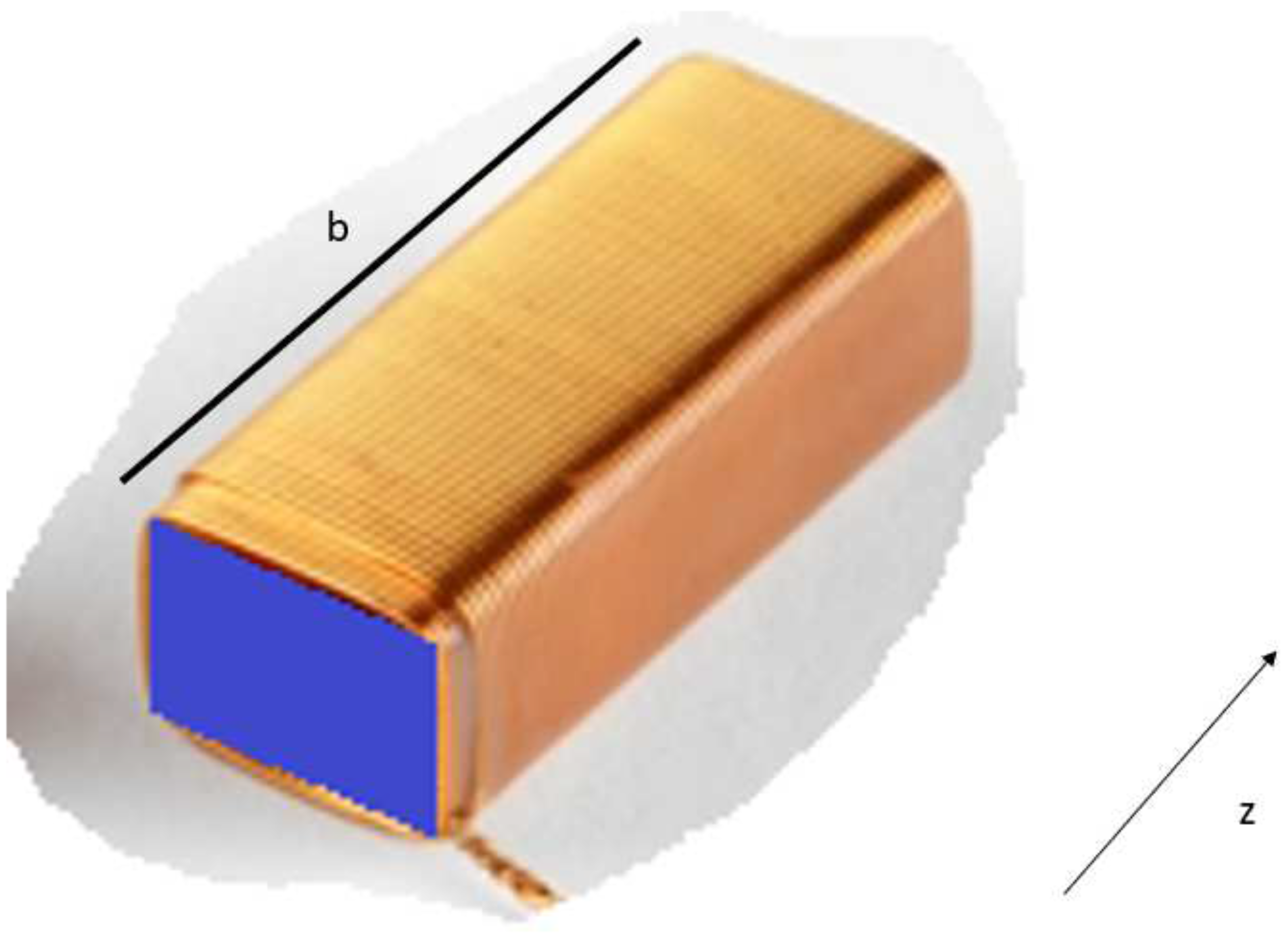
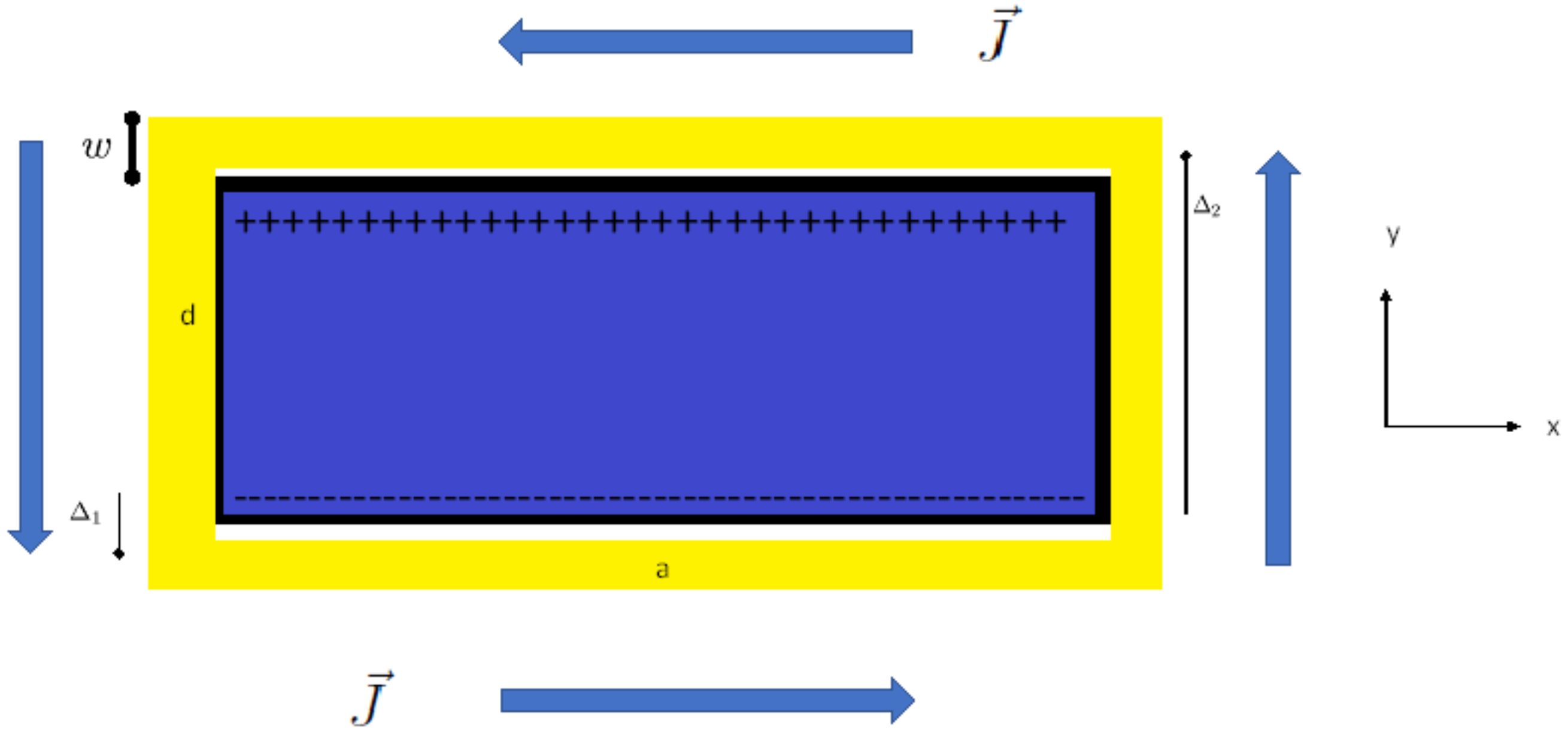
| Car | Rocket Size Engine | Giant Cube | Units | |
|---|---|---|---|---|
| a | 6 | 200 | 1000 | m |
| b | 2 | 10 | 1000 | m |
| d | 1 | 10 | 1000 | m |
| w | 0.2 | 0.4 | 0.4 | m |
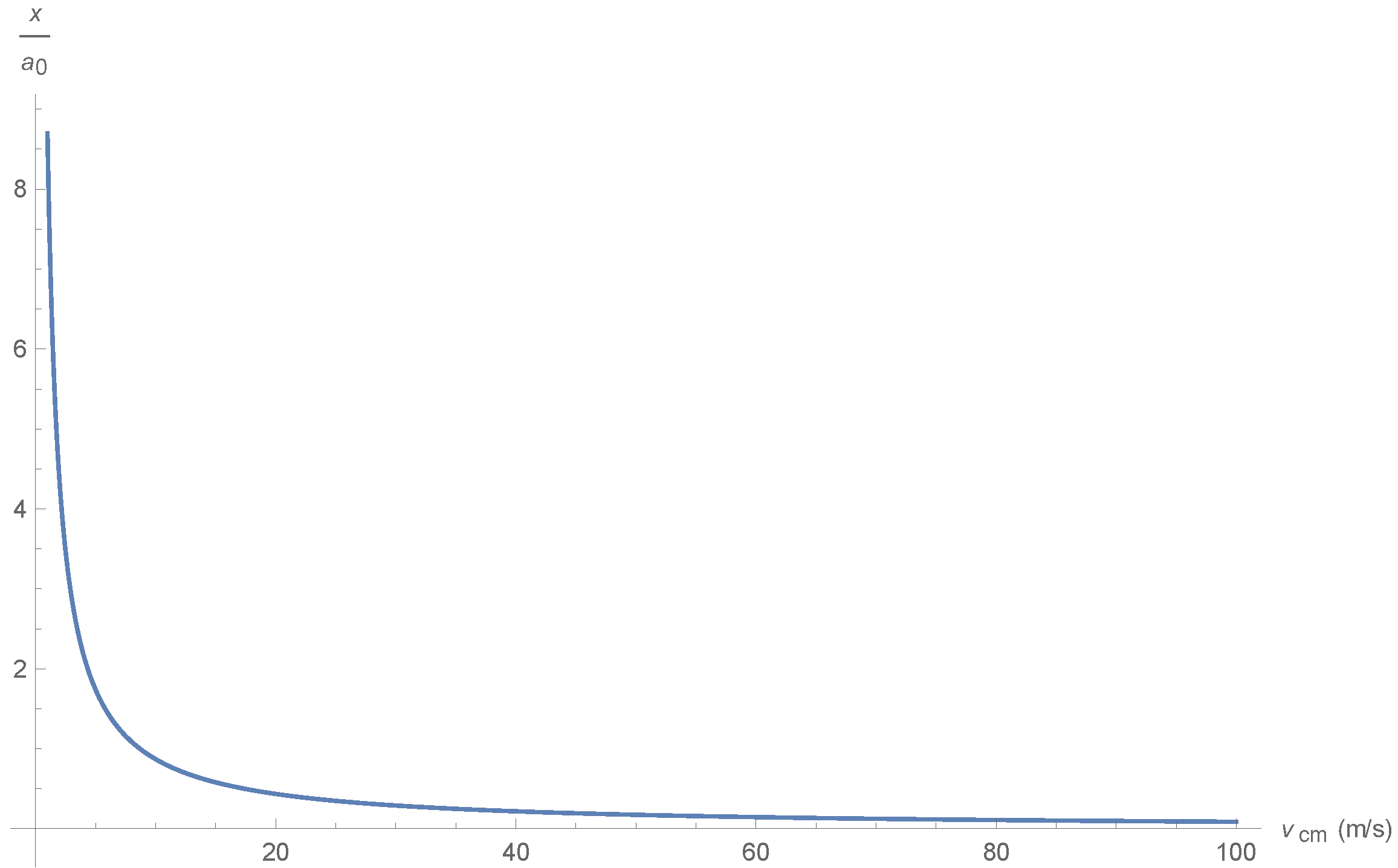
| 0.3 | 868 | kg m/s |
Disclaimer/Publisher’s Note: The statements, opinions and data contained in all publications are solely those of the individual author(s) and contributor(s) and not of MDPI and/or the editor(s). MDPI and/or the editor(s) disclaim responsibility for any injury to people or property resulting from any ideas, methods, instructions or products referred to in the content. |
© 2023 by the author. Licensee MDPI, Basel, Switzerland. This article is an open access article distributed under the terms and conditions of the Creative Commons Attribution (CC BY) license (https://creativecommons.org/licenses/by/4.0/).
Share and Cite
Yahalom, A. Implementing a Relativistic Motor over Atomic Scales. Symmetry 2023, 15, 1613. https://doi.org/10.3390/sym15081613
Yahalom A. Implementing a Relativistic Motor over Atomic Scales. Symmetry. 2023; 15(8):1613. https://doi.org/10.3390/sym15081613
Chicago/Turabian StyleYahalom, Asher. 2023. "Implementing a Relativistic Motor over Atomic Scales" Symmetry 15, no. 8: 1613. https://doi.org/10.3390/sym15081613
APA StyleYahalom, A. (2023). Implementing a Relativistic Motor over Atomic Scales. Symmetry, 15(8), 1613. https://doi.org/10.3390/sym15081613