The Landweber Iterative Regularization Method for Identifying the Unknown Source of Caputo-Fabrizio Time Fractional Diffusion Equation on Spherically Symmetric Domain

Abstract

In this article, the inverse problem for identifying the space-dependent source of time fractional diffusion equation on a spherically symmetric domain with Caputo–Fabrizio fractional derivative is discussed. This problem is a typical ill-posed problem and the Landweber iterative regularization method is used to obtain the approximation solution. The convergent error estimates under a priori regularization parameter choice rule and a posteriori regularization parameter choice rule are given, respectively. The numerical examples are given to show the effectiveness of the Landweber iterative regularization method.

1. Introduction

Fractional calculus equation has the advantages of simple modeling, clear physical meaning, accurate description and so on, so they are used in many fields such as hydrogeology, fluid mechanics, biomedicine, etc. There are many ways to define fractional derivatives [1], and the fractional derivative selected in this article is a Caputo–Fabrizio fractional derivative [2], which was first given by M. Caputo and M. Fabrizio in 2015. The Caputo fractional derivative is

$$D_t^{\alpha }f(t)=\frac{1}{\mathsf{\Gamma }(1-\alpha )}{\int }_a^t{f}^{\prime }(\tau )\frac{1}{{(t-\tau )}^{\alpha }}d\tau ,$$

where $\alpha \in [0,1]$, $a\in (-\infty ,t)$, $f\in H^1(a,b)$, $b>a$, if ${(t-\tau )}^{-\alpha }$ is changed to $e^{-\frac{\alpha }{1-\alpha }t}$ and $\frac{1}{\mathsf{\Gamma }(1-\alpha )}$ is changed to $\frac{M(\alpha )}{1-\alpha }$, then we can obtain the other fractional derivative as follows:

$${}_{CF}{D}_{0,t}^{\alpha }f(t)=\frac{M(\alpha )}{1-\alpha }{\int }_a^t{f}^{\prime }(\tau )e^{-\frac{\alpha (t-\tau )}{1-\alpha }}d\tau ,$$

here, $M(\alpha )$ is a normalization function and satisfies $M(0)=M(1)=1$. ${}_{CF}{D}_{0,t}^{\alpha }$ is called the Caputo–Fabrizio fractional derivative. So, many scholars have studied this type of fractional derivative [3,4,5,6,7]. In [8], let $a=0$, the Caputo–Fabrizio fractional derivative’s Laplace transform is as follows:

$$L{[}_{CF}{D}_{0,t}^{\alpha }f(t)]=\frac{pL[f(t)]-f(0)}{p+\alpha (1-p)},$$

and the case of order $1<\beta \le 2$ is considered in [9].

When we use the fractional diffusion equation model to solve a practical problem, some parameters in the fractional diffusion equation model are unknown, such as the initial value or source term. We need some additional measure data to identify these unknown parameters, which leads to the inverse problem of fractional diffusion equation. Inverse problem of fractional diffusion equation is an interdisciplinary and frontier science. In [10,11,12,13,14], the inverse problem of the Cauchy problem of the fractional diffusion equation is considered by different regularization methods. In [15,16,17,18,19], the initial value of the fractional diffusion equation is identified by different regularization methods. In [20,21,22,23,24], the unknown source of the fractional diffusion equation is discriminated by different regularization methods. In [25,26,27], the inverse problem of the fractional diffusion equation on a columnar symmetric domain are studied. In [28,29,30,31], the inverse problem of the fractional diffusion equation on a spherically symmetric domain are studied. In Figure 1 and Figure 2, the grain of a spherically symmetric domain diffusion geometry is shown, which is actually consistent with laboratory measurements of helium diffusion from a physical point of view from apatite. As a consequence of radiogenic production and diffusive loss, $u(r,t)$ denotes the concentration of helium and depends on the spherically radius r and t.

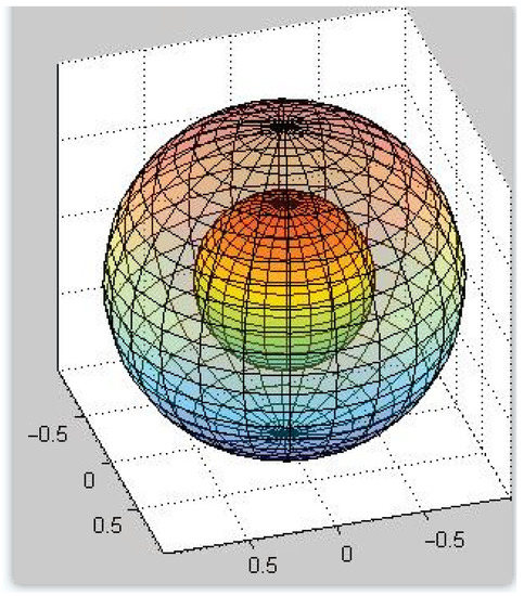
Figure 1. The three-dimensional model for the spherically symmetrix domain.

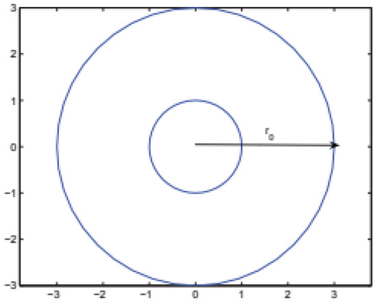
Figure 2. The two-dimensional model for the spherically symmetrix domain.

In this article, the time fractional diffusion equation on the spherically symmetric domain with the Caputo–Fabrizio fractional derivative is considered as follows:

$$\left\{\begin{array}{cc}{}_{CF}{D}_{0,t}^{\alpha }u(r,t)-\frac{2}{r}{u}_r(r,t)-u_{rr}(r,t)=f(r),\hfill & 0<r<r_0,0<t<T,\hfill \\ u(r_0,t)=0,\hfill & 0\le t\le T,\hfill \\ u(r,0)=a(r),\hfill & 0\le r\le r_0,\hfill \\ u(r,T)=g(r),\hfill & 0\le r\le r_0,\hfill \\ \underset{r\to 0}{lim}u(r,t)bounded,\hfill & 0\le t\le T,\hfill \end{array}\right.$$

(1)

here, $r_0$ is the radius of the circle, $T>0$ is a final time, and ${}_{CF}{D}_{0,t}^{\alpha }$ is the Caputo–Fabrizio operator for the fractional derivative of the order $\alpha$ defined by

$${}_{CF}{D}_{0,t}^{\alpha }u(t)=\frac{M(\alpha )}{1-\alpha }{\int }_0^t{e}^{\frac{-\alpha }{1-\alpha }(t-z)}\frac{\partial u(z)}{\partial z}dz,t\ge 0,0<\alpha <1.$$

In problem (1), space-dependent source $f(r)$ is unknown, and the additional condition $u(x,T)=g(r)$ is used to identify $f(r)$. In practice, there are errors in the exact data $g(r)$, $\delta >0$ represents the error of measurement. We assume that the exact data $g(r)$ and the measured data $g^{\delta }(r)$ satisfy

$$\parallel g^{\delta }{(r)-g(r)\parallel }_{L^2[0,r_0;r^2]}\le \delta ,$$

(2)

where, ${\parallel ·\parallel }_{L^2[0,r_0;r^2]}$ is the $L^2[0,r_0;r^2]$ norm. $L^2[0,r_0;r^2]$ represents the Hilbert space with weight $r^2$ in the interval $[0,r_0]$ of the Lebesgue measurable function. $(·,·)$ represents the inner product of $L^2[0,r_0;r^2]$ space, and $\parallel ·\parallel$ represents the norm of $L^2[0,r_0;r^2]$ space, it is defined as follows:

$$\parallel f\parallel =({\int }_0^{r_0}{r}^2{|f(r)|}^2{dr)}^{\frac{1}{2}}.$$

The novelty of this paper is as follows: firstly, the new kind fractional derivative, i.e., Caputo–Fabrizio fractional derivative, is considered. Secondly, we consider the inverse problem for identifying the unknown source for the high dimensional fractional diffusion equation, not the one-dimensional fractional diffusion equation. Thirdly, two different regularization parameter choice rules are given, i.e., the priori regularization parameter choice rule and the posteriori regularization parameter choice rule.

The structure of this article is defined as follows: Section 2 lists some preliminary knowledge. In Section 3, we find the solution of problem (1), analyze its ill-posedness, and give the conditional stability result. In Section 4, we give the Landweber iterative regularization method, obtain the problem (1), and give the error estimations. In Section 5, we design the numerical algorithms to verify the validity of the regularization method. Finally, in Section 6, we give the conclusion.

2. Preliminary Results

In order to more conveniently solve this inverse problem, we give the following definition. For $p>0$, define

$$H^p=\{\mu \in L^2[0,r_0;r^2]|\sum _{n=1}^{\infty }{(n^2)}^p|(\mu ,R_n){|}^2<\infty \},$$

where, $(·,·)$ is the inner product in $L^2[0,r_0;r^2]$. Thus, $H^p$ is a Hilbert space with the norm

$${\parallel \mu \parallel }_{H^p}=(\sum _{n=1}^{\infty }{(n^2)}^p|(\mu ,R_n){{|}^2)}^{\frac{1}{2}}.$$

Theorem 1.

For $0<\alpha <1$, we have

$$C_2{n}^2\le \frac{{(\frac{n\pi }{r_0})}^2+(1-\alpha ){(\frac{n\pi }{r_0})}^4}{1+(1-\alpha ){(\frac{n\pi }{r_0})}^2-e^{\frac{-\alpha {(\frac{n\pi }{r_0})}^{2}T}{1+(1-\alpha ){(\frac{n\pi }{r_0})}^2}}}\le C_1{n}^2,$$

(3)

where, $C_1$ and $C_2$ are normal numbers.

Proof. 

Because $e^{\frac{-\alpha {(\frac{n\pi }{r_0})}^{2}T}{1+(1-\alpha ){(\frac{n\pi }{r_0})}^2}}<1$, we can obtain

$$\begin{array}{cc}\hfill \frac{{(\frac{n\pi }{r_0})}^2+(1-\alpha ){(\frac{n\pi }{r_0})}^4}{1+(1-\alpha ){(\frac{n\pi }{r_0})}^2-e^{\frac{-\alpha {(\frac{n\pi }{r_0})}^{2}T}{1+(1-\alpha ){(\frac{n\pi }{r_0})}^2}}}& \le \frac{{(\frac{n\pi }{r_0})}^2+(1-\alpha ){(\frac{n\pi }{r_0})}^4}{1+(1-\alpha ){(\frac{n\pi }{r_0})}^2-1}\hfill \\ \hfill & =\frac{1+(1-\alpha ){(\frac{n\pi }{r_0})}^2}{1-\alpha }\hfill \\ \hfill & \le (\frac{1}{1-\alpha }+\frac{{\pi }^2}{r_0^2})n^2\hfill \\ \hfill & =C_1{n}^2,\hfill \end{array}$$

where, $C_1=\frac{1}{1-\alpha }+\frac{{\pi }^2}{r_0^2}$.

Because $e^{\frac{-\alpha {(\frac{n\pi }{r_0})}^{2}T}{1+(1-\alpha ){(\frac{n\pi }{r_0})}^2}}>0$, we obtain

$$\begin{array}{cc}\hfill \frac{{(\frac{n\pi }{r_0})}^2+(1-\alpha ){(\frac{n\pi }{r_0})}^4}{1+(1-\alpha ){(\frac{n\pi }{r_0})}^2-e^{\frac{-\alpha {(\frac{n\pi }{r_0})}^{2}T}{1+(1-\alpha ){(\frac{n\pi }{r_0})}^2}}}& \ge \frac{{(\frac{n\pi }{r_0})}^2+(1-\alpha ){(\frac{n\pi }{r_0})}^4}{1+(1-\alpha ){(\frac{n\pi }{r_0})}^2}\hfill \\ \hfill & ={(\frac{n\pi }{r_0})}^2\hfill \\ \hfill & =C_2{n}^2,\hfill \end{array}$$

where, $C_2=\frac{{\pi }^2}{r_0^2}$. So,

$$C_2{n}^2\le \frac{{(\frac{n\pi }{r_0})}^2+(1-\alpha ){(\frac{n\pi }{r_0})}^4}{1+(1-\alpha ){(\frac{n\pi }{r_0})}^2-e^{\frac{-\alpha {(\frac{n\pi }{r_0})}^{2}T}{1+(1-\alpha ){(\frac{n\pi }{r_0})}^2}}}\le C_1{n}^2.$$

□

Lemma 1.

If $0\le h\le 1$, $0\le \rho \le 1$, $n\ge 1$, then we obtain

$$\frac{1-{(1-h)}^n}{h^{\rho }}\le n^{\rho }.$$

(4)

Proof. 

If $0\le h\le 1,0\le \rho \le 1,n\ge 1$, we can obtain

$$\begin{array}{cc}\hfill \frac{1-{(1-h)}^n}{h^{\rho }}& \le {(\frac{1-{(1-h)}^n}{h})}^{\rho }\hfill \\ \hfill & \le n^{\rho }.\hfill \end{array}$$

□

3. The Ill-Posedness of Problem (1) and the Conditional Stability Result

The exact solution of the problem (1) is obtained by the method of separation of variables and the Laplace transformation as follows:

$$\begin{array}{cc}\hfill u(x,t)=& \sum _{n=1}^{\infty }(\frac{1+(1-\alpha ){(\frac{n\pi }{r_0})}^2-e^{\frac{-\alpha {(\frac{n\pi }{r_0})}^{2}t}{1+(1-\alpha ){(\frac{n\pi }{r_0})}^2}}}{{(\frac{n\pi }{r_0})}^2+(1-\alpha ){(\frac{n\pi }{r_0})}^4}{f}_n\hfill \\ \hfill & +\frac{1}{1+(1-\alpha ){(\frac{n\pi }{r_0})}^2}{e}^{\frac{-\alpha {(\frac{n\pi }{r_0})}^{2}t}{1+(1-\alpha ){(\frac{n\pi }{r_0})}^2}}{a}_n)R_n(r),\hfill \end{array}$$

where, $R_n(r)=\frac{\sqrt{2}n\pi }{\sqrt[3]{r_0}}\frac{sin(\frac{n\pi r}{r_0})}{\frac{n\pi r}{r_0}}$, $n=1,2,\cdots$ is a standard orthogonal system with weight $r^2$ in the $[0,r_0]$, and it is complete in the class of square-integrable functions in $[0,r_0]$, $a_n=(a(r),R_n(r))$ and $f_n=(f(r),R_n(r))$ are Fourier coefficients.

Utilizing $g(r)=u(r,T)$, we can obtain

$$\begin{array}{cc}\hfill g(r)=& \sum _{n=1}^{\infty }(\frac{1+(1-\alpha ){(\frac{n\pi }{r_0})}^2-e^{\frac{-\alpha {(\frac{n\pi }{r_0})}^{2}T}{1+(1-\alpha ){(\frac{n\pi }{r_0})}^2}}}{{(\frac{n\pi }{r_0})}^2+(1-\alpha ){(\frac{n\pi }{r_0})}^4}{f}_n\hfill \\ \hfill & +\frac{1}{1+(1-\alpha ){(\frac{n\pi }{r_0})}^2}{e}^{\frac{-\alpha {(\frac{n\pi }{r_0})}^{2}T}{1+(1-\alpha ){(\frac{n\pi }{r_0})}^2}}{a}_n)R_n(r),\hfill \end{array}$$

and let

$$\begin{array}{c}\hfill g_n:=\frac{1+(1-\alpha ){(\frac{n\pi }{r_0})}^2-e^{\frac{-\alpha {(\frac{n\pi }{r_0})}^{2}T}{1+(1-\alpha ){(\frac{n\pi }{r_0})}^2}}}{{(\frac{n\pi }{r_0})}^2+(1-\alpha ){(\frac{n\pi }{r_0})}^4}{f}_n+\frac{1}{1+(1-\alpha ){(\frac{n\pi }{r_0})}^2}{e}^{\frac{-\alpha {(\frac{n\pi }{r_0})}^{2}T}{1+(1-\alpha ){(\frac{n\pi }{r_0})}^2}}{a}_n,\end{array}$$

where, $g_n=(g(r),R_n(r))$ is Fourier coefficient. Let

$$h(r):=g(r)-\sum _{n=1}^{\infty }\frac{1}{1+(1-\alpha ){(\frac{n\pi }{r_0})}^2}{e}^{\frac{-\alpha {(\frac{n\pi }{r_0})}^{2}T}{1+(1-\alpha ){(\frac{n\pi }{r_0})}^2}}{a}_n{R}_n(r).$$

Then,

$$h_n=g_n-\frac{1}{1+(1-\alpha ){(\frac{n\pi }{r_0})}^2}{e}^{\frac{-\alpha {(\frac{n\pi }{r_0})}^{2}T}{1+(1-\alpha ){(\frac{n\pi }{r_0})}^2}}{a}_n,$$

and

$$h(r)=\sum _{n=1}^{\infty }\frac{1+(1-\alpha ){(\frac{n\pi }{r_0})}^2-e^{\frac{-\alpha {(\frac{n\pi }{r_0})}^{2}T}{1+(1-\alpha ){(\frac{n\pi }{r_0})}^2}}}{{(\frac{n\pi }{r_0})}^2+(1-\alpha ){(\frac{n\pi }{r_0})}^4}{f}_n{R}_n(r),$$

$$h_n=\frac{1+(1-\alpha ){(\frac{n\pi }{r_0})}^2-e^{\frac{-\alpha {(\frac{n\pi }{r_0})}^{2}T}{1+(1-\alpha ){(\frac{n\pi }{r_0})}^2}}}{{(\frac{n\pi }{r_0})}^2+(1-\alpha ){(\frac{n\pi }{r_0})}^4}{f}_n.$$

It is easy to know that

$$f_n=\frac{{(\frac{n\pi }{r_0})}^2+(1-\alpha ){(\frac{n\pi }{r_0})}^4}{1+(1-\alpha ){(\frac{n\pi }{r_0})}^2-e^{\frac{-\alpha {(\frac{n\pi }{r_0})}^{2}T}{1+(1-\alpha ){(\frac{n\pi }{r_0})}^2}}}{h}_n.$$

(5)

$$f(r)=\sum _{n=1}^{\infty }\frac{{(\frac{n\pi }{r_0})}^2+(1-\alpha ){(\frac{n\pi }{r_0})}^4}{1+(1-\alpha ){(\frac{n\pi }{r_0})}^2-e^{\frac{-\alpha {(\frac{n\pi }{r_0})}^{2}T}{1+(1-\alpha ){(\frac{n\pi }{r_0})}^2}}}{h}_n{R}_n(r).$$

(6)

In order to find the unknown source $f(r)$, we define the linear operator $K:f\to h$, and solve the following integral equation:

$$(Kf)(r)={\int }_0^{r_0}k(r,\xi )f(\xi )d\xi =h(r),$$

$k(r,\xi )$, which is the kernel function as defined by

$$k(r,\xi )=\sum _{n=1}^{\infty }\frac{1+(1-\alpha ){(\frac{n\pi }{r_0})}^2-e^{\frac{-\alpha {(\frac{n\pi }{r_0})}^{2}T}{1+(1-\alpha ){(\frac{n\pi }{r_0})}^2}}}{{(\frac{n\pi }{r_0})}^2+(1-\alpha ){(\frac{n\pi }{r_0})}^4}{R}_n(r)R_n(\xi ).$$

Since $k(r,\xi )=k(\xi ,r)$, K is a self-adjoint operator. According to [32], $K:L^2[0,r_0;r^2]\to L^2[0,r_0;r^2]$ is a compact operator, so (1) is an ill-posed problem.

Let $K^{*}$ be the self-adjoint operator of K. Because $R_n(r)$ is a set of standard orthogonal systems with weight $r^2$ in the $L^2[0,r_0;r^2]$, then

$$K^{*}K{R}_n(\xi )=(\frac{1+(1-\alpha ){(\frac{n\pi }{r_0})}^2-e^{\frac{-\alpha {(\frac{n\pi }{r_0})}^{2}T}{1+(1-\alpha ){(\frac{n\pi }{r_0})}^2}}}{{(\frac{n\pi }{r_0})}^2+(1-\alpha ){(\frac{n\pi }{r_0})}^4}{)}^2{R}_n(\xi ).$$

Thus, ${\sigma }_n=\frac{1+(1-\alpha ){(\frac{n\pi }{r_0})}^2-e^{\frac{-\alpha {(\frac{n\pi }{r_0})}^{2}T}{1+(1-\alpha ){(\frac{n\pi }{r_0})}^2}}}{{(\frac{n\pi }{r_0})}^2+(1-\alpha ){(\frac{n\pi }{r_0})}^4}$ is the singular value of K.

Suppose $f(r)\in H^p$ satisfies a priori bound condition

$${\parallel f\parallel }_{H^p}\le E,$$

(7)

and ${\parallel f\parallel }_{H^p}$ is computed by

$${\parallel f\parallel }_{H^p}={(\sum _{n=1}^{\infty }{(n^2)}^p{f}_n^2)}^{\frac{1}{2}},$$

where, p and E are normal numbers.

Theorem 2.

Suppose $f(r)\in H^p$ and satisfies (7), so we obtain

$$\parallel f\parallel \le C_3{E}^{\frac{2}{p+2}}{\parallel g\parallel }^{\frac{p}{p+2}},$$

(8)

where, $C_3=C_1^{\frac{p}{p+2}}$.

Proof. 

Using (6) and the Hölder inequality, we obtain

$$\begin{array}{cc}\hfill {\parallel f\parallel }^2& =\parallel \sum _{n=1}^{\infty }\frac{{(\frac{n\pi }{r_0})}^2+(1-\alpha ){(\frac{n\pi }{r_0})}^4}{1+(1-\alpha ){(\frac{n\pi }{r_0})}^2-e^{\frac{-\alpha {(\frac{n\pi }{r_0})}^{2}T}{1+(1-\alpha ){(\frac{n\pi }{r_0})}^2}}}{h}_n{R}_n{(r)\parallel }^2\hfill \\ \hfill & =\sum _{n=1}^{\infty }(\frac{{(\frac{n\pi }{r_0})}^2+(1-\alpha ){(\frac{n\pi }{r_0})}^4}{1+(1-\alpha ){(\frac{n\pi }{r_0})}^2-e^{\frac{-\alpha {(\frac{n\pi }{r_0})}^{2}T}{1+(1-\alpha ){(\frac{n\pi }{r_0})}^2}}}{h}_n{)}^2\hfill \\ \hfill & =\sum _{n=1}^{\infty }(\frac{{(\frac{n\pi }{r_0})}^2+(1-\alpha ){(\frac{n\pi }{r_0})}^4}{1+(1-\alpha ){(\frac{n\pi }{r_0})}^2-e^{\frac{-\alpha {(\frac{n\pi }{r_0})}^{2}T}{1+(1-\alpha ){(\frac{n\pi }{r_0})}^2}}}{)}^2{h}_n^{\frac{4}{p+2}}{h}_n^{\frac{2p}{p+2}}\hfill \\ \hfill & =\sum _{n=1}^{\infty }(\frac{{(\frac{n\pi }{r_0})}^2+(1-\alpha ){(\frac{n\pi }{r_0})}^4}{1+(1-\alpha ){(\frac{n\pi }{r_0})}^2-e^{\frac{-\alpha {(\frac{n\pi }{r_0})}^{2}T}{1+(1-\alpha ){(\frac{n\pi }{r_0})}^2}}}{)}^p{f}_n^2{)}^{\frac{2}{p+2}}{h}_n^{\frac{2p}{p+2}}\hfill \\ \hfill & \le (\sum _{n=1}^{\infty }((1+(1-\alpha ){(\frac{n\pi }{r_0})}^2)e^{\frac{\alpha {(\frac{n\pi }{r_0})}^{2}T}{1+(1-\alpha ){(\frac{n\pi }{r_0})}^2}}{)}^p{f}_n^2{)}^{\frac{2}{p+2}}(\sum _{n=1}^{\infty }{h}_n^2{)}^{\frac{p}{p+2}}.\hfill \end{array}$$

Using (3) and (7), we can obtain

$$\begin{array}{cc}\hfill \sum _{n=1}^{\infty }((1+(1-\alpha ){(\frac{n\pi }{r_0})}^2)e^{\frac{\alpha {(\frac{n\pi }{r_0})}^{2}T}{1+(1-\alpha ){(\frac{n\pi }{r_0})}^2}}{)}^p{f}_n^2& \le \sum _{n=1}^{\infty }{(C_1{n}^2)}^p{f}_n^2\hfill \\ \hfill & =C_1^p\sum _{n=1}^{\infty }{(n^2)}^p{f}_n^2\le C_1^p{E}^2,\hfill \end{array}$$

therefore,

$${\parallel f\parallel }^2\le {(C_1^p{E}^2)}^{\frac{2}{p+2}}{(\sum _{n=1}^{\infty }{h}_n^2)}^{\frac{p}{p+2}}.$$

Thus,

$$\parallel f\parallel \le C_3{E}^{\frac{2}{p+2}}{\parallel h\parallel }^{\frac{p}{p+2}},$$

where, $C_3=C_1^{\frac{p}{p+2}}$. □

4. The Regularization Method and the Error Estimations

In this section, we use the Landweber iterative regularization method to solve the problem (1). Replacing the operator equation $Kf=h$ with operator equation $f=(I-d{K}^{*}K)a+d{K}^{*}h$, we obtain the iterative formula as follows:

$$f^{0,\delta }(r)=0,f^{m,\delta }(r)=(I-d(K^{*}K))f^{m-1,\delta }(r)+d{K}^{*}{h}^{\delta }(r),$$

where, $m=1,2,3,\cdots$ is the iteration steps and the regularization parameter. d is the relaxation factor and satisfies $0<d<\frac{1}{{\parallel K\parallel }^2}$. ${\sigma }_n$ is the singular value of K. Then, we obtain

$$0<d(\frac{1+(1-\alpha ){(\frac{n\pi }{r_0})}^2-e^{\frac{-\alpha {(\frac{n\pi }{r_0})}^{2}T}{1+(1-\alpha ){(\frac{n\pi }{r_0})}^2}}}{{(\frac{n\pi }{r_0})}^2+(1-\alpha ){(\frac{n\pi }{r_0})}^4}{)}^2<1$$

.

The operator $R_m:L^2[0,r_0;r^2]\to L^2[0,r_0;r^2]$ can be expressed as follows:

$$R_m=d\sum _{n=0}^{m-1}{(I-d{K}^{*}K)}^n{K}^{*}.$$

Through simple calculation, we obtain

$$f^{m,\delta }(r)=R_m{h}^{\delta }(r)=d\sum _{n=0}^{m-1}{(I-d{K}^{*}K)}^n{K}^{*}{h}^{\delta }(r).$$

Thus, the Landweber iterative regularization solution is obtained as follows:

$$f^{m,\delta }(r)=\sum _{n=1}^{\infty }\frac{1-(1-d(\frac{1+(1-\alpha ){(\frac{n\pi }{r_0})}^2-e^{\frac{-\alpha {(\frac{n\pi }{r_0})}^{2}T}{1+(1-\alpha ){(\frac{n\pi }{r_0})}^2}}}{{(\frac{n\pi }{r_0})}^2+(1-\alpha ){(\frac{n\pi }{r_0})}^4}{)}^2{)}^m}{\frac{1+(1-\alpha ){(\frac{n\pi }{r_0})}^2-e^{\frac{-\alpha {(\frac{n\pi }{r_0})}^{2}T}{1+(1-\alpha ){(\frac{n\pi }{r_0})}^2}}}{{(\frac{n\pi }{r_0})}^2+(1-\alpha ){(\frac{n\pi }{r_0})}^4}}{h}_n^{\delta }{R}_n(r),$$

(9)

where, $h_n^{\delta }=(h^{\delta }(r),R_n(r))$.

The Landweber regularization solution without error is given as follows:

$$f^m(r)=\sum _{n=1}^{\infty }\frac{1-(1-d(\frac{1+(1-\alpha ){(\frac{n\pi }{r_0})}^2-e^{\frac{-\alpha {(\frac{n\pi }{r_0})}^{2}T}{1+(1-\alpha ){(\frac{n\pi }{r_0})}^2}}}{{(\frac{n\pi }{r_0})}^2+(1-\alpha ){(\frac{n\pi }{r_0})}^4}{)}^2{)}^m}{\frac{1+(1-\alpha ){(\frac{n\pi }{r_0})}^2-e^{\frac{-\alpha {(\frac{n\pi }{r_0})}^{2}T}{1+(1-\alpha ){(\frac{n\pi }{r_0})}^2}}}{{(\frac{n\pi }{r_0})}^2+(1-\alpha ){(\frac{n\pi }{r_0})}^4}}{h}_n{R}_n(r).$$

(10)

4.1. A Priori Error Estimation

Theorem 3.

$f(r)$ and $f^{m,\delta }(r)$ are given by (6) and (9). Assume (2) and (7) hold, then if we select

$$m=\left[{(\frac{E}{\delta })}^{\frac{4}{p+2}}\right],$$

(11)

we obtain

$$\parallel f^{m,\delta }(r)-f(r)\parallel \le C_4{E}^{\frac{2}{p+2}}{\delta }^{\frac{p}{p+2}},$$

(12)

where $C_4=d^{\frac{1}{2}}+{(\frac{C_1^{2}p}{d})}^{\frac{p}{4}}$, $\left[{(\frac{E}{\delta })}^{\frac{4}{p+2}}\right]$ is the largest integer not larger than ${(\frac{E}{\delta })}^{\frac{4}{p+2}}$.

Proof. 

By the triangle inequality, we can obtain

$$\parallel f^{m,\delta }(r)-f(r)\parallel \le \parallel f^{m,\delta }(r)-f^m(r)\parallel +\parallel f^m(r)-f(r)\parallel .$$

By (2), (9), (10) and inequality (4), we have

$$\begin{array}{cc}\hfill \parallel f^{m,\delta }(r)-f^m{(r)\parallel }^2& =\sum _{n=1}^{\infty }(\frac{1-(1-d(\frac{1+(1-\alpha ){(\frac{n\pi }{r_0})}^2-e^{\frac{-\alpha {(\frac{n\pi }{r_0})}^{2}T}{1+(1-\alpha ){(\frac{n\pi }{r_0})}^2}}}{{(\frac{n\pi }{r_0})}^2+(1-\alpha ){(\frac{n\pi }{r_0})}^4}{)}^2{)}^m}{\frac{1+(1-\alpha ){(\frac{n\pi }{r_0})}^2-e^{\frac{-\alpha {(\frac{n\pi }{r_0})}^{2}T}{1+(1-\alpha ){(\frac{n\pi }{r_0})}^2}}}{{(\frac{n\pi }{r_0})}^2+(1-\alpha ){(\frac{n\pi }{r_0})}^4}}{)}^2{(h_n^{\delta }-h_n)}^2\hfill \\ \hfill & =\sum _{n=1}^{\infty }(d^{\frac{1}{2}}\frac{1-(1-(d^{\frac{1}{2}}\frac{1+(1-\alpha ){(\frac{n\pi }{r_0})}^2-e^{\frac{-\alpha {(\frac{n\pi }{r_0})}^{2}T}{1+(1-\alpha ){(\frac{n\pi }{r_0})}^2}}}{{(\frac{n\pi }{r_0})}^2+(1-\alpha ){(\frac{n\pi }{r_0})}^4}{)}^2{)}^m}{((d^{\frac{1}{2}}\frac{1+(1-\alpha ){(\frac{n\pi }{r_0})}^2-e^{\frac{-\alpha {(\frac{n\pi }{r_0})}^{2}T}{1+(1-\alpha ){(\frac{n\pi }{r_0})}^2}}}{{(\frac{n\pi }{r_0})}^2+(1-\alpha ){(\frac{n\pi }{r_0})}^4}{)}^2{)}^{\frac{1}{2}}}{)}^2{(h_n^{\delta }-h_n)}^2\hfill \\ \hfill & \le {(d^{\frac{1}{2}}{m}^{\frac{1}{2}})}^2\sum _{n=1}^{\infty }{(h_n^{\delta }-h_n)}^2\hfill \\ \hfill & ={(d^{\frac{1}{2}}{m}^{\frac{1}{2}}\delta )}^2.\hfill \end{array}$$

Thus,

$$\parallel f^{m,\delta }(r)-f^m(r)\parallel \le d^{\frac{1}{2}}{m}^{\frac{1}{2}}\delta .$$

(13)

With (10) and (7), we have

$$\begin{array}{cc}\hfill \parallel f^m{(r)-f(r)\parallel }^2& =\sum _{n=1}^{\infty }(\frac{-(1-d(\frac{1+(1-\alpha ){(\frac{n\pi }{r_0})}^2-e^{\frac{-\alpha {(\frac{n\pi }{r_0})}^{2}T}{1+(1-\alpha ){(\frac{n\pi }{r_0})}^2}}}{{(\frac{n\pi }{r_0})}^2+(1-\alpha ){(\frac{n\pi }{r_0})}^4}{)}^2{)}^m}{\frac{1+(1-\alpha ){(\frac{n\pi }{r_0})}^2-e^{\frac{-\alpha {(\frac{n\pi }{r_0})}^{2}T}{1+(1-\alpha ){(\frac{n\pi }{r_0})}^2}}}{{(\frac{n\pi }{r_0})}^2+(1-\alpha ){(\frac{n\pi }{r_0})}^4}}{h}_n{)}^2\hfill \\ \hfill & =\sum _{n=1}^{\infty }((1-d(\frac{1+(1-\alpha ){(\frac{n\pi }{r_0})}^2-e^{\frac{-\alpha {(\frac{n\pi }{r_0})}^{2}T}{1+(1-\alpha ){(\frac{n\pi }{r_0})}^2}}}{{(\frac{n\pi }{r_0})}^2+(1-\alpha ){(\frac{n\pi }{r_0})}^4}{)}^2{)}^m{f}_n{)}^2\hfill \\ \hfill & =\sum _{n=1}^{\infty }((1-d(\frac{1+(1-\alpha ){(\frac{n\pi }{r_0})}^2-e^{\frac{-\alpha {(\frac{n\pi }{r_0})}^{2}T}{1+(1-\alpha ){(\frac{n\pi }{r_0})}^2}}}{{(\frac{n\pi }{r_0})}^2+(1-\alpha ){(\frac{n\pi }{r_0})}^4}{)}^2{)}^m{f}_n{(n^2)}^{\frac{p}{2}}{(n^2)}^{-\frac{p}{2}}{)}^2\hfill \\ \hfill & \le (\underset{n\ge 1}{sup}((1-d(\frac{1+(1-\alpha ){(\frac{n\pi }{r_0})}^2-e^{\frac{-\alpha {(\frac{n\pi }{r_0})}^{2}T}{1+(1-\alpha ){(\frac{n\pi }{r_0})}^2}}}{{(\frac{n\pi }{r_0})}^2+(1-\alpha ){(\frac{n\pi }{r_0})}^4}{)}^2{)}^m{(n^2)}^{-\frac{p}{2}}{)}^2)E^2\hfill \\ \hfill & \le (\underset{n\ge 1}{sup}((1-d(\frac{1}{C_1{n}^2}{)}^2{)}^m{n}^{-p}{)}^2)E^2.\hfill \end{array}$$

Let $A(t)=(1-d(\frac{1}{C_1{n}^2}{)}^2{)}^m{n}^{-p}$. Suppose $n_0$ satisfies $A^{\prime }(n_0)=0$, we can obtain

$$n_0={(\frac{d(4m+p)}{C_1^{2}p})}^{\frac{1}{4}}.$$

Thus,

$$\begin{array}{cc}\hfill A(n)& \le A(n_0)\hfill \\ \hfill & ={(1-\frac{p}{4m+p})}^m{(\frac{d(4m+p)}{C_1^{2}p})}^{-\frac{p}{4}}\le {(\frac{d(4m+p)}{C_1^{2}p})}^{-\frac{p}{4}}\hfill \\ \hfill & \le {(\frac{C_1^{2}p}{d})}^{\frac{p}{4}}{(4m+p)}^{-\frac{p}{4}}\le {(\frac{C_1^{2}p}{d})}^{\frac{p}{4}}{(m+1)}^{-\frac{p}{4}}.\hfill \end{array}$$

Then,

$$\parallel f^m(r)-f(r)\parallel \le {(\frac{C_1^{2}p}{d})}^{\frac{p}{4}}{(m+1)}^{-\frac{p}{4}}E.$$

(14)

Using (13) and (14), we have

$$\parallel f^{m,\delta }(r)-f(r)\parallel \le d^{\frac{1}{2}}{m}^{\frac{1}{2}}\delta +{(\frac{C_1^{2}p}{d})}^{\frac{p}{4}}{(m+1)}^{-\frac{p}{4}}E.$$

Selecting the regularization parameter $m=\left[{(\frac{E}{\delta })}^{\frac{4}{p+2}}\right]$, we have

$$\parallel f^{m,\delta }(r)-f(r)\parallel \le C_4{E}^{\frac{2}{p+2}}{\delta }^{\frac{p}{p+2}},$$

where, $C_4=d^{\frac{1}{2}}+{(\frac{C_1^{2}p}{d})}^{\frac{p}{4}}$. □

4.2. A Posteriori Error Estimation

Next, give the a posteriori regularization choice rule based on the Discrepancy Principle, and obtain the convergence error estimate under a posteriori regularization choice rule.

Let $\tau >1$ be a given constant. For $\parallel h^{\delta }\parallel \ge \tau \delta$, choose $m=m(\delta )\in {\mathbb{N}}_0$ such that m satisfies

$$\parallel K{f}^{m,\delta }(r)-h^{\delta }(r)\parallel \le \tau \delta$$

(15)

appears for the first time, iteration stops.

Lemma 2.

Suppose $\rho (m)=\parallel K{f}^{m,\delta }(r)-h^{\delta }(r)\parallel$, so we obtain

(1)

$\rho (m)$ is a continuous function.

(2)

$\underset{m\to 0}{lim}\rho (m)=\parallel h^{\delta }\parallel$.

(3)

$\underset{m\to +\infty }{lim}\rho (m)=0;$

(4)

For any $m\in (0,+\infty )$, $\rho (m)$ is a strictly decreasing function.

Lemma 3.

Let $\tau >1$ and (15) hold, then m satisfies

$$m\le \frac{C_1^2(p+2)}{2C_2^{\frac{4}{p+2}}d}{(\frac{E}{(\tau -1)\delta })}^{\frac{4}{p+2}}.$$

(16)

Proof. 

According to (9), we have

$$R_{m}h=\sum _{n=1}^{\infty }\frac{1-(1-d(\frac{1+(1-\alpha ){(\frac{n\pi }{r_0})}^2-e^{\frac{-\alpha {(\frac{n\pi }{r_0})}^{2}T}{1+(1-\alpha ){(\frac{n\pi }{r_0})}^2}}}{{(\frac{n\pi }{r_0})}^2+(1-\alpha ){(\frac{n\pi }{r_0})}^4}{)}^2{)}^m}{\frac{1+(1-\alpha ){(\frac{n\pi }{r_0})}^2-e^{\frac{-\alpha {(\frac{n\pi }{r_0})}^{2}T}{1+(1-\alpha ){(\frac{n\pi }{r_0})}^2}}}{{(\frac{n\pi }{r_0})}^2+(1-\alpha ){(\frac{n\pi }{r_0})}^4}}{h}_n{R}_n(r).$$

So,

$$\parallel K{R}_m{h-h\parallel }^2=\sum _{n=1}^{\infty }(1-d(\frac{1+(1-\alpha ){(\frac{n\pi }{r_0})}^2-e^{\frac{-\alpha {(\frac{n\pi }{r_0})}^{2}T}{1+(1-\alpha ){(\frac{n\pi }{r_0})}^2}}}{{(\frac{n\pi }{r_0})}^2+(1-\alpha ){(\frac{n\pi }{r_0})}^4}{)}^2{)}^{2m}{h}_n^2.$$

Because of $|1-d(\frac{1+(1-\alpha ){(\frac{n\pi }{r_0})}^2-e^{\frac{-\alpha {(\frac{n\pi }{r_0})}^{2}T}{1+(1-\alpha ){(\frac{n\pi }{r_0})}^2}}}{{(\frac{n\pi }{r_0})}^2+(1-\alpha ){(\frac{n\pi }{r_0})}^4}{)}^2|<1$, so $\parallel K{R}_{m-1}-I\parallel \le 1$. Using (15), we can obtain

$$\begin{array}{cc}\hfill \parallel K{R}_{m-1}h-h\parallel & =\parallel K{R}_{m-1}h-h+K{R}_{m-1}{h}^{\delta }-K{R}_{m-1}{h}^{\delta }+h^{\delta }-h^{\delta }\parallel \hfill \\ \hfill & \ge \parallel K{R}_{m-1}{h}^{\delta }-h^{\delta }\parallel -\parallel (K{R}_{m-1}-I)(h-h^{\delta })\parallel \hfill \\ \hfill & \ge \tau \delta -\parallel K{R}_{m-1}-I\parallel \delta \hfill \\ \hfill & \ge (\tau -1)\delta .\hfill \end{array}$$

On the other side, using (7), we can obtain

$$\begin{array}{cc}\hfill \parallel K{R}_{m-1}h-h\parallel =& \parallel \sum _{n=1}^{\infty }(1-(1-d(\frac{1+(1-\alpha ){(\frac{n\pi }{r_0})}^2-e^{\frac{-\alpha {(\frac{n\pi }{r_0})}^{2}T}{1+(1-\alpha ){(\frac{n\pi }{r_0})}^2}}}{{(\frac{n\pi }{r_0})}^2+(1-\alpha ){(\frac{n\pi }{r_0})}^4}{)}^2{)}^{m-1})h_n{R}_n(r)\hfill \\ \hfill & -\sum _{n=1}^{\infty }{h}_n{R}_n(r)\parallel \hfill \\ \hfill =& \sum _{n=1}^{\infty }(1-d(\frac{1+(1-\alpha ){(\frac{n\pi }{r_0})}^2-e^{\frac{-\alpha {(\frac{n\pi }{r_0})}^{2}T}{1+(1-\alpha ){(\frac{n\pi }{r_0})}^2}}}{{(\frac{n\pi }{r_0})}^2+(1-\alpha ){(\frac{n\pi }{r_0})}^4}{)}^2{)}^{m-1}|h_n|\hfill \\ \hfill =& \sum _{n=1}^{\infty }(1-d(\frac{1+(1-\alpha ){(\frac{n\pi }{r_0})}^2-e^{\frac{-\alpha {(\frac{n\pi }{r_0})}^{2}T}{1+(1-\alpha ){(\frac{n\pi }{r_0})}^2}}}{{(\frac{n\pi }{r_0})}^2+(1-\alpha ){(\frac{n\pi }{r_0})}^4}{)}^2{)}^{m-1}\hfill \\ \hfill & ·|\frac{1+(1-\alpha ){(\frac{n\pi }{r_0})}^2-e^{\frac{-\alpha {(\frac{n\pi }{r_0})}^{2}T}{1+(1-\alpha ){(\frac{n\pi }{r_0})}^2}}}{{(\frac{n\pi }{r_0})}^2+(1-\alpha ){(\frac{n\pi }{r_0})}^4}||f_n{(n^2)}^{\frac{p}{2}}|{(n^2)}^{-\frac{p}{2}}\hfill \\ \hfill \le & (\underset{n\ge 1}{sup}J(n))E,\hfill \end{array}$$

here $J(n)=(1-d(\frac{1+(1-\alpha ){(\frac{n\pi }{r_0})}^2-e^{\frac{-\alpha {(\frac{n\pi }{r_0})}^{2}T}{1+(1-\alpha ){(\frac{n\pi }{r_0})}^2}}}{{(\frac{n\pi }{r_0})}^2+(1-\alpha ){(\frac{n\pi }{r_0})}^4}{)}^2{)}^{m-1}|\frac{1+(1-\alpha ){(\frac{n\pi }{r_0})}^2-e^{\frac{-\alpha {(\frac{n\pi }{r_0})}^{2}T}{1+(1-\alpha ){(\frac{n\pi }{r_0})}^2}}}{{(\frac{n\pi }{r_0})}^2+(1-\alpha ){(\frac{n\pi }{r_0})}^4}|{(n^2)}^{-\frac{p}{2}}$. So

$$(\tau -1)\delta \le J(n)E.$$

(17)

Using (3), we can obtain $J(n)\le {(1-d{(\frac{1}{C_1{n}^2})}^2)}^{m-1}\frac{1}{C_2{n}^2}{(n^2)}^{-\frac{p}{2}}$.

Let $B(n)={(1-d{(\frac{1}{C_1{n}^2})}^2)}^{m-1}\frac{1}{C_2{n}^2}{(n^2)}^{-\frac{p}{2}}$, assume $n_0$ satisfies $B^{\prime }(n_0)=0$, then $n_0={(\frac{d(4(m-1)+(p+2))}{C_1^2(p+2)})}^{\frac{1}{4}}$, thus

$$\begin{array}{cc}\hfill B(n)& \le B(n_0)=(1-\frac{p+2}{4(m-1)+(p+2)}{)}^{m-1}\frac{1}{C_2}(\frac{d(4(m-1)+(p+2))}{C_1^2(p+2)}{)}^{-\frac{p+2}{4}}\hfill \\ \hfill & \le (\frac{d{C}_2^{\frac{4}{p+2}}(4(m-1)+(p+2))}{C_1^2(p+2)}{)}^{-\frac{p+2}{4}}\hfill \\ \hfill & =(\frac{C_1^2(p+2)}{d{C}_2^{\frac{4}{p+2}}(2m+2m-4+(p+2))}{)}^{\frac{p+2}{4}}\hfill \\ \hfill & =(\frac{C_1^2(p+2)}{2C_2^{\frac{4}{p+2}}dm}{)}^{\frac{p+2}{4}}.\hfill \end{array}$$

Therefore,

$$J(n)\le (\frac{C_1^2(p+2)}{2C_2^{\frac{4}{p+2}}d}{)}^{\frac{p+2}{4}}{m}^{-\frac{p+2}{4}}.$$

(18)

Using (17) and (18), we have

$$(\tau -1)\delta \le (\frac{C_1^2(p+2)}{2C_2^{\frac{4}{p+2}}d}{)}^{\frac{p+2}{4}}{m}^{-\frac{p+2}{4}}E.$$

Thus,

$$m\le \frac{C_1^2(p+2)}{2C_2^{\frac{4}{p+2}}d}{(\frac{E}{(\tau -1)\delta })}^{\frac{4}{p+2}}.$$

□

Theorem 4.

The exact solution $f(r)$ is given by (6) and the regularization solution $f^{m,\delta }(r)$ is given by (9). Assume (7) and (2) hold, the regularization parameter m is chosen by (15), then

$$\parallel f^{m,\delta }(r)-f(r)\parallel \le (C_5+C_3{(\tau +1)}^{\frac{p}{p+2}})E^{\frac{2}{p+2}}{\delta }^{\frac{p}{p+2}},$$

(19)

where $C_5=(\frac{C_1^2(p+2)}{2C_2^{\frac{4}{p+2}}}{)}^{\frac{1}{2}}{(\frac{1}{\tau -1})}^{\frac{2}{p+2}}$.

Proof. 

Through the triangle inequality, we obtain

$$\parallel f^{m,\delta }(r)-f(r)\parallel \le \parallel f^{m,\delta }(r)-f^m(r)\parallel +\parallel f^m(r)-f(r)\parallel .$$

Using (13) and (16), we have

$$\begin{array}{cc}\hfill \parallel f^{m,\delta }(r)-f^m(r)\parallel & \le d^{\frac{1}{2}}{m}^{\frac{1}{2}}\delta \hfill \\ \hfill & \le {(\frac{C_1^2(p+2)}{2C_2^{\frac{4}{p+2}}})}^{\frac{1}{2}}{(\frac{E}{(\tau -1)\delta })}^{\frac{2}{p+2}}\delta \hfill \\ \hfill & =C_5{E}^{\frac{2}{p+2}}{\delta }^{\frac{p}{p+2}},\hfill \end{array}$$

here $C_5={(\frac{C_1^2(p+2)}{2C_2^{\frac{4}{p+2}}})}^{\frac{1}{2}}{(\frac{1}{\tau -1})}^{\frac{2}{p+2}}$.

For $\parallel f^m(r)-f(r)\parallel$, we know

$$\begin{array}{cc}\hfill K(f^m(r)-f(r))=& \sum _{n=1}^{\infty }-(1-d(\frac{1+(1-\alpha ){(\frac{n\pi }{r_0})}^2-e^{\frac{-\alpha {(\frac{n\pi }{r_0})}^{2}T}{1+(1-\alpha ){(\frac{n\pi }{r_0})}^2}}}{{(\frac{n\pi }{r_0})}^2+(1-\alpha ){(\frac{n\pi }{r_0})}^4}{)}^2{)}^m{h}_n{R}_n(r)\hfill \\ \hfill =& \sum _{n=1}^{\infty }-(1-d(\frac{1+(1-\alpha ){(\frac{n\pi }{r_0})}^2-e^{\frac{-\alpha {(\frac{n\pi }{r_0})}^{2}T}{1+(1-\alpha ){(\frac{n\pi }{r_0})}^2}}}{{(\frac{n\pi }{r_0})}^2+(1-\alpha ){(\frac{n\pi }{r_0})}^4}{)}^2{)}^m(h_n-h_n^{\delta })R_n(r)\hfill \\ \hfill & +\sum _{n=1}^{\infty }-(1-d(\frac{1+(1-\alpha ){(\frac{n\pi }{r_0})}^2-e^{\frac{-\alpha {(\frac{n\pi }{r_0})}^{2}T}{1+(1-\alpha ){(\frac{n\pi }{r_0})}^2}}}{{(\frac{n\pi }{r_0})}^2+(1-\alpha ){(\frac{n\pi }{r_0})}^4}{)}^2{)}^m{h}_n^{\delta }{R}_n(r).\hfill \end{array}$$

Using (2) and (15), we have

$$\begin{array}{cc}\hfill \parallel K(f^m(r)-f(r))\parallel & \le \delta +\tau \delta \hfill \\ \hfill & =(\tau +1)\delta .\hfill \end{array}$$

Using (7), we obtain

$$\begin{array}{cc}\hfill \parallel f^m{(r)-f(r)\parallel }_{H^p}=& (\sum _{n=1}^{\infty }(1-d(\frac{1+(1-\alpha ){(\frac{n\pi }{r_0})}^2-e^{\frac{-\alpha {(\frac{n\pi }{r_0})}^{2}T}{1+(1-\alpha ){(\frac{n\pi }{r_0})}^2}}}{{(\frac{n\pi }{r_0})}^2+(1-\alpha ){(\frac{n\pi }{r_0})}^4}{)}^2{)}^{2m}\hfill \end{array}$$

$$\begin{array}{cc}\hfill & ·(\frac{{(\frac{n\pi }{r_0})}^2+(1-\alpha ){(\frac{n\pi }{r_0})}^4}{1+(1-\alpha ){(\frac{n\pi }{r_0})}^2-e^{\frac{-\alpha {(\frac{n\pi }{r_0})}^{2}T}{1+(1-\alpha ){(\frac{n\pi }{r_0})}^2}}}{h}_n{)}^2{(n^2)}^p{)}^{\frac{1}{2}}\hfill \\ \hfill \le & {(\sum _{n=1}^{\infty }{(n^2)}^p{f}_n^2)}^{\frac{1}{2}}\hfill \\ \hfill \le & E.\hfill \end{array}$$

According to (8), we obtain

$$\begin{array}{cc}\hfill \parallel f^m(r)-f(r)\parallel & \le C_3{E}^{\frac{2}{p+2}}{((\tau +1)\delta )}^{\frac{p}{p+2}}\hfill \\ \hfill & =C_3{(\tau +1)}^{\frac{p}{p+2}}{E}^{\frac{2}{p+2}}{\delta }^{\frac{p}{p+2}}.\hfill \end{array}$$

So,

$$\begin{array}{cc}\hfill \parallel f^{m,\delta }(r)-f(r)\parallel & \le C_5{E}^{\frac{2}{p+2}}{\delta }^{\frac{p}{p+2}}+C_3{(\tau +1)}^{\frac{p}{p+2}}{E}^{\frac{2}{p+2}}{\delta }^{\frac{p}{p+2}}\hfill \\ \hfill & =(C_5+C_3{(\tau +1)}^{\frac{p}{p+2}})E^{\frac{2}{p+2}}{\delta }^{\frac{p}{p+2}}.\hfill \end{array}$$

□

5. Numerical Examples

In this section, we use three numerical examples to show the validity of the Landweber iterative regularization method. First, through the known function $f(r)$, we solve the direct problem to obtain the final value data $g(r)$, then consider the inverse problem, use additional data $g(r)$ to obtain regularization solution $f^{m,\delta }(r)$.

$$\left\{\begin{array}{cc}{}_{CF}{D}_{0,t}^{\alpha }u(r,t)-\frac{2}{r}{u}_r(r,t)-u_{rr}(r,t)=f(r),\hfill & 0<r<r_0,0<t<T,\hfill \\ u(r_0,t)=0,\hfill & 0\le t\le T,\hfill \\ u(r,0)=a(r),\hfill & 0\le r\le r_0,\hfill \\ \underset{r\to 0}{lim}u(r,t)bounded,\hfill & 0\le t\le T.\hfill \end{array}\right.$$

(20)

The finite difference method is used to solve (20). Let $r_0=\pi$, the time variable is $\Delta t=T/N$, the space variable is $\Delta r=\pi /M$. Grid points in the time interval are marked as $t_n=n\Delta t$, $n=1,2,\dots ,N$, and the space interval are marked as $r_i=i\Delta r$, $i=1,2,\dots ,M$. The approach value of the unknown function is $u_i^n\approx u(r_i,t_n)$.

Based on [33,34], a discrete approach to the Caputo–Fabrizio fractional derivative is computed by

$${}_{CF}{D}_{0,t}^{\alpha }u(r_i,t_n)\approx \frac{1}{\alpha ·\Delta t}\sum _{j=1}^n(u_i^{n-j+1}-u_i^{n-j})M_j,0<\alpha <1,$$

here $i=1,2,3,\cdots ,M-1$, $n=1,2,\cdots ,N$, $M_j=exp(-\frac{(j-1)\alpha }{1-\alpha })-exp(-\frac{j\alpha }{1-\alpha })$, the space derivatives is computed approximately by

$$u_r(r_i,t_n)\approx \frac{u_{i+1}^n-u_i^n}{\Delta r},$$

$$u_{rr}(r_i,t_n)\approx \frac{u_{i-1}^n-2u_i^n+u_{i+1}^n}{{(\Delta r)}^2}.$$

Denote $U^n={(U_1^n,U_2^n,\cdots ,U_{M-1}^n)}^T$, $a={(a(r_1),a(r_2),\cdots ,a(r_{M-1}))}^T$, $f={(f(r_1),f(r_2),\cdots ,f(r_{M-1}))}^T$, we obtain the iterative scheme

$$\begin{array}{cc}\hfill A{U}^1=& \frac{1}{\alpha ·\Delta t}{M}_{1}a+f,\hfill \\ \hfill A{U}^n=& \frac{1}{\alpha ·\Delta t}({\beta }_1{U}^{n-1}+{\beta }_2{U}^{n-2}+\cdots {\beta }_{n-1}{U}^1+M_{n}a)+f,\hfill \end{array}$$

where, ${\beta }_j=M_j-M_{j+1}$, $A_{(M-1)\times (M-1)}$ is a tridiagonal matrix as follows:

$$A=\left(\begin{array}{cc}\frac{M_1}{\alpha ·\Delta t}+y_1\frac{1}{{(\Delta r)}^2}& -z_1\frac{1}{{(\Delta r)}^2}\\ -\frac{1}{{(\Delta r)}^2}& \frac{M_1}{\alpha ·\Delta t}+y_2\frac{1}{{(\Delta r)}^2}& -z_2\frac{1}{{(\Delta r)}^2}\\ \ddots & \ddots & \ddots \\ & & -\frac{1}{{(\Delta r)}^2}& \frac{M_1}{\alpha ·\Delta t}+y_{M-1}\frac{1}{{(\Delta r)}^2}\end{array}\right),$$

where, $y_i=2+\frac{2}{i}$, $i=1,2,\cdots ,M-1$, $z_j=1+\frac{2}{j}$, $j=1,2,\cdots ,M-2$.

The measured data $g(r)$ have errors, so add random disturbance to $g(r)$ to generate noise data $g^{\delta }(r)$ as follows:

$$g^{\delta }=g+\epsilon g(2randn(size(g))-1),$$

(21)

The function $randn(·)$ generates a random number array with a mean equal to 0, and a variance equal to 1. $\epsilon$ is the relative error level, and the absolute error level $\delta$ is

$$\delta =\sqrt{\frac{1}{M+1}\sum _{i=1}^{M+1}{(g_i-g_i^{\delta })}^2}.$$

(22)

However, in practical problem application, the prior bound of the exact solution cannot be accurately obtained. A priori regularization parameter depends on the smooth condition of the exact solution, it is difficult to obtain accurately. Therefore, in the following numerical experiment, the numerical result is only given under a posteriori regularization parameter choice rule.

In the numerical experiments, take $\tau =1.1$, $N=50$, $M=100$, $T=1$, $p=2$, and $a(r)=0$.

Example 1.

Take the smooth function

$$f(r)=e^r·sin(6r),0\le r\le \pi .$$

Example 2.

Take the piecewise smooth function

$$f(r)=\left\{\begin{array}{cc}2,\hfill & 0\le r<\frac{\pi }{3},\hfill \\ 0,\hfill & \frac{\pi }{3}\le r<\frac{2\pi }{3},\hfill \\ -2,\hfill & \frac{2\pi }{3}\le r\le \pi .\hfill \end{array}\right.$$

Example 3.

Take the non-smooth function

$$f(r)=\left\{\begin{array}{cc}0,\hfill & 0\le r<\frac{\pi }{4},\hfill \\ 4r-\pi ,\hfill & \frac{\pi }{4}\le r<\frac{\pi }{2},\hfill \\ -4r+3\pi ,\hfill & \frac{\pi }{2}\le r<\frac{3\pi }{4},\hfill \\ 0,\hfill & \frac{3\pi }{4}\le r\le \pi .\hfill \end{array}\right.$$

Figure 3 indicates the Landweber iterative regularization solution $f^{m,\delta }(r)$ and the exact solution $f(r)$ for Example 1 under various $\epsilon =0.1,0.05,0.01$ for $\alpha =0.1$, $\alpha =0.4$ and $\alpha =0.7$.

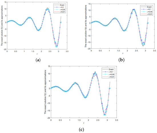
Figure 3. The comparison between the Landweber regularization solution $f^{m,\delta }(r)$ given by a posteriori parameter choice rule and the exact solution $f(r)$ for Example 1, (a) $\alpha =0.1$, (b) $\alpha =0.4$, (c) $\alpha =0.7$.

Figure 4 indicates the Landweber iterative regularization solution $f^{m,\delta }(r)$ and the exact solution $f(r)$ for Example 2 under various $\epsilon =0.1,0.05,0.01$ for $\alpha =0.1$, $\alpha =0.4$ and $\alpha =0.7$

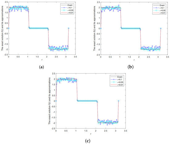
Figure 4. The comparison between the Landweber regularization solution $f^{m,\delta }(r)$ given by a posteriori parameter choice rule and the exact solution $f(r)$ for Example 2, (a) $\alpha =0.1$, (b) $\alpha =0.4$, (c) $\alpha =0.7$.

Figure 5 indicates the Landweber iterative regularization solution $f^{m,\delta }(r)$ and the exact solution $f(r)$ for Example 3 under various $\epsilon =0.1,0.05,0.01$ for $\alpha =0.1$, $\alpha =0.4$ and $\alpha =0.7$.

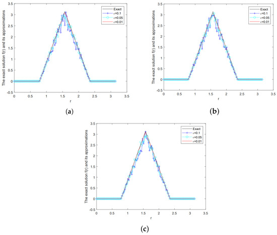
Figure 5. The comparison between the Landweber regularization solution $f^{m,\delta }(r)$ given by a posteriori parameter choice rule and the exact solution $f(r)$ for Example 3, (a) $\alpha =0.1$, (b) $\alpha =0.4$, (c) $\alpha =0.7$.

From Figure 3, Figure 4 and Figure 5, when $\epsilon$ is fixed, if $\alpha$ is smaller, the fitting results of the exact solution and the Landweber iterative regularization solution is better. On the contrary, if $\alpha$ is bigger, the ill-posed problem will be strengthened, the fitting results of the exact solution and the Landweber iterative regularization solution is worse. When $\alpha$ is fixed, if $\epsilon$ is smaller, the fitting results of the exact solution and the Landweber iterative regularization solution is better.

From Figure 3, Figure 4 and Figure 5, we can also see that the numerical solutions of Examples 2 and 3 are unsatisfactory than those of Example 1. Because in Examples 2 and 3, the exact solutions are non-smooth and discontinuous functions, the recover data near the non-smooth and discontinuous points are not accurate. This is the well-known Gibbs phenomenon. But for the ill-posed problem, we consider that the outcomes in Figure 4 and Figure 5 are sensible.

Through the above numerical examples, it can be seen that the Landweber iterative regularization method is effective and stable.

6. Conclusions

We propose the inverse problem for identifying the unknown source of the time fractional diffusion equation on a spherically symmetric domain with a Caputo–Fabrizio fractional derivative. We use the method of separation of variables and the Laplace transformation to calculate the exact solution of this problem. By analyzing the exact solution, we find this problem is ill-posed. We use the Landweber iterative regularization method to obtain the regularization solution and give the error estimates between the exact solution and the regularization solution. Through numerical examples, we proved that Landweber iterative regularization method is effective. In the future, we will discuss the inverse problem for identifying the initial value for the time fractional diffusion equation on spherically symmetric domain with a Caputo–Fabrizio fractional derivative. Moreover, we will discuss to identify simultaneously the unknown source and the initial value for the time fractional diffusion equation on spherically symmetric domain with a Caputo–Fabrizio fractional derivative.

References

- Derbazi, C.; Baitiche, Z.; Zada, A. Existence and uniqueness of positive solutions for fractional relaxation equation in terms of ψ-Caputo fractional derivative. Int. J. Nonlin. Sci. Num. 2023, 24, 633–643. [Google Scholar] [CrossRef]
- Caputo, M.; Fabrizio, M. A new definition of fractional derivative without singular kernel. Progr. Fract. Differ. Appl. 2015, 1, 73–85. [Google Scholar]
- Losada, J.; Nieto, J.J. Properties of a new fractional derivative without singular kernel. Progr. Fract. Differ. Appl. 2015, 1, 87–92. [Google Scholar]
- Caputo, M.; Fabrizio, M. Applications of new time and spatial fractional derivatives with exponential kernels. Progr. Fract. Differ. Appl. 2016, 2, 1–11. [Google Scholar] [CrossRef]
- Al-khedhairi, A. Dynamical analysis and chaos synchronization of a fraction-order novel financial model based on Caputo-Fabrizio derivative. Eur. Phys. J. Plus 2019, 134, 532. [Google Scholar]
- Tuan, N.H.; Zhou, Y. Well-posedness of an initial value problem for fractional diffusion equation with Caputo-Fabrizio derivative. Chaos Solut. Fract. 2020, 138, 109966. [Google Scholar] [CrossRef]
- Baleanu, D.; Jajarmi, A.; Mohammadi, H.; Rezapour, S. A new study on the mathematical modelling of human liver with Caputo-Fabrizio derivative. Chaos Solut. Fract. 2020, 134, 109705. [Google Scholar] [CrossRef]
- Mirza, I.A.; Vieru, D. Fundametal solutions to advection-diffusion equation with time-fractional Caputo-Fabrizio derivative. Comput. Math. Appl. 2017, 73, 1–10. [Google Scholar] [CrossRef]
- Al-salti, N.; Sadarangani, E. On a differential equation with Caputo-Fabrizio fractional derivative of order 1<β≤2 and application to mass-spring-damper system. Progr. Fract. Differ. Appl. 2016, 2, 257–263. [Google Scholar]
- Dou, F.F.; Hon, Y.C. Kernel-based approximation for Cauchy problem of the time-fractional diffusion equation. Eng. Anal. Bound. Elem. 2012, 36, 1344–1352. [Google Scholar] [CrossRef]
- Xiong, X.T.; Zhao, L.P.; Hon, Y.C. Stability estimate and the modified regularization method for a Cauchy problem of the fractional diffusion equation. J. Comput. Appl. Math. 2014, 5, 016. [Google Scholar] [CrossRef]
- Povstenko, Y.; Klekot, J. Fundamental solution to the cauchy problem for the time-fractional advection-diffusion equation. J. Appl. Math. Comput. Mech. 2014, 13, 95–102. [Google Scholar] [CrossRef]
- Anatoly, N.K. Cauchy problem for fractional diffusion-wave equations with variable coefficients. Appl. Anal. 2014, 93, 2211–2242. [Google Scholar]
- Wei, T.; Zhang, Z.Q. Stable numerical solution to a Cauchy problem for a time fractional diffusion equation. Eng. Anal. Bound. Elem. 2014, 40, 128–137. [Google Scholar] [CrossRef]
- Yang, F.; Zhang, Y.; Li, X.X. Landweber iterative method for identifying the initial value problem of the time-space fractional diffusion-wave equation. Numer. Algor. 2020, 83, 1509–1530. [Google Scholar] [CrossRef]
- Xian, J.; Wei, T. Determination of the initial data in a time-fractional diffusion-wave problem by a final time data. Comput. Math. Appl. 2019, 78, 2525–2540. [Google Scholar] [CrossRef]
- Zhang, Y.; Wei, T.; Zhang, Y.X. Simultaneous inversion of two initial values for a time-fractional diffusion-wave equation. Numer. Methods Part. Differ. Equ. 2021, 37, 24–43. [Google Scholar] [CrossRef]
- Thach, T.N.; Can, N.H.; Tri, V.V. Identifying the initial state for a parabolic diffusion from their time averages with fractional derivative. Math. Method Appl. Sci. 2021, 1, 7751–7766. [Google Scholar]
- Jiang, S.Z.; Liao, K.F.; Wei, T. Inversion of the Initial Value for a Time-Fractional Diffusion-Wave Equation by Boundary Data. Comput. Math. Appl. 2020, 20, 109–120. [Google Scholar] [CrossRef]
- Wei, T.; Sun, L.L.; Li, Y.S. Uniqueness for an inverse space-dependent source term in a multi-dimensional time-fractional diffusion equation. Appl. Math. Lett. 2016, 61, 108–113. [Google Scholar] [CrossRef]
- Li, Y.S.; Wei, T. An inverse time-dependent source problem for a time-space fractional diffusion equation. Appl. Math. Comput. 2018, 336, 257–271. [Google Scholar]
- Wei, T.; Li, X.L.; Li, Y.S. An inverse time-dependent source problem for a time-fractional diffusion equation. Inverse Probl. 2016, 32, 085003. [Google Scholar] [CrossRef]
- Tian, W.; Li, C.; Deng, W.; Wu, Y. Regularization methods for unknown source in space fractional diffusion equation. Math. Comput. Simul. 2012, 85, 45–56. [Google Scholar]
- Tuan, N.H.; Le, D.L.; Nguyen, V.T. Regularization of an inverse source problem for a time fractional diffusion equation. Appl. Math. Model 2016, 40, 8244–8264. [Google Scholar]
- Yang, F.; Sun, Y.R.; Li, X.X.; Huang, C.Y. The quasi-boundary regularization value method for identifying the initial value of heat equation on a columnar symmetric domain. Numer. Algor. 2019, 82, 623–639. [Google Scholar] [CrossRef]
- Wang, L.; Stynes, M. An α-robust finite difference method for a time-fractional radially symmetric diffusion problem. Comput. Math. Appl. 2021, 97, 386–393. [Google Scholar] [CrossRef]
- Chen, Y.G.; Yang, F.; Li, X.X.; Li, D.G. The Fractional Tikhonov regularization method to identify the initial value of the nonhomogeneous time-fractional diffusion equation on a columnar symmetrical domain. Symmetry 2022, 14, 1633. [Google Scholar] [CrossRef]
- Yang, F.; Wang, N.; Li, X.X. Landweber iterative method for an inverse source problem of time-fractional diffusion-wave equation on spherically symmetric domain. Appl. Anal. Comput. 2020, 10, 514–529. [Google Scholar] [CrossRef]
- Long, L.D.; Van, H.T.K.; Binh, H.D.; Saadati, R. On backward problem for fractional spherically symmetric diffusion equation with observation data of nonlocal type. Adv. Differ. Equ. 2021, 1, 445. [Google Scholar] [CrossRef]
- Yang, S.; Xiong, X.T.; Nie, Y. Iterated fractional Tikhonov regularization method for solving the spherically symmetric backward time-fractional diffusion equation. Appl. Numer. Math. 2021, 160, 217–241. [Google Scholar] [CrossRef]
- Cheng, W.; Liu, Y.L.; Yang, F. A Modified Regularization Method for a Spherically Symmetric Inverse Heat Conduction Problem. Symmetry 2022, 14, 2102. [Google Scholar] [CrossRef]
- Zhang, Z.Q.; Wei, T. Identifying an unknown source in time-fractional diffusion equation by a truncation method. Appl. Math. Comput. 2013, 219, 5972–5983. [Google Scholar] [CrossRef]
- Atangana, A.; Alqahtani, R.T. Numerical approximation of the space-time Caputo-Fabrizio fractional derivative and qpplication to groundwater pollution equation. Adv. Differ. Equ. 2016, 2016, 156. [Google Scholar] [CrossRef]
- Akman, T.; Yildiz, B.; Baleanu, D. New discretization of Caputo-Fabrizio derivative. Comput. Appl. Math. 2018, 37, 3307–3333. [Google Scholar] [CrossRef]
Disclaimer/Publisher’s Note: The statements, opinions and data contained in all publications are solely those of the individual author(s) and contributor(s) and not of MDPI and/or the editor(s). MDPI and/or the editor(s) disclaim responsibility for any injury to people or property resulting from any ideas, methods, instructions or products referred to in the content. |
© 2023 by the authors. Licensee MDPI, Basel, Switzerland. This article is an open access article distributed under the terms and conditions of the Creative Commons Attribution (CC BY) license (https://creativecommons.org/licenses/by/4.0/).