Article

High-Performance Intermediate-Frequency Balanced Homodyne Detector for Local Local Oscillator Continuous-Variable Quantum Key Distribution

1
State Key Laboratory of Information Photonics and Optical Communications, Beijing University of Posts and Telecommunications, Beijing 100876, China
2
School of Cyberspace Security, Beijing University of Posts and Telecommunications, Beijing 100876, China
3
State Key Laboratory of Advanced Optical Communication Systems and Networks, School of Electronics, and Center for Quantum Information Technology, Peking University, Beijing 100871, China
*
Authors to whom correspondence should be addressed.
Symmetry 2023, 15(7), 1314; https://doi.org/10.3390/sym15071314
Submission received: 18 May 2023 / Revised: 19 June 2023 / Accepted: 20 June 2023 / Published: 27 June 2023
(This article belongs to the Section Physics)

Abstract

:
In the continuous-variable quantum key distribution (CV-QKD) system with a local local oscillator (LLO), the center frequency of the sender and the receiver’s source are not exactly the same and a certain frequency drift exists over time, resulting in the frequency of the signal received near the intermediate frequency. Therefore, the LLO system needs an intermediate-frequency balanced homodyne detector (BHD), which needs better symmetry of the arms of the BHD, to obtain the less-common mode noise. Moreover, the traditional intermediate-frequency receiver in classical communication is not available in the CV-QKD system because of the low quantum-to-classical noise ratio. In view of this, in this paper, we construct a broadband intermediate-frequency BHD based on ratio frequency and integrated circuit technology, whose bandwidth can exceed 270 MHz and whose quantum-to-classical noise ratio can reach 14.9 dB. Meanwhile, the BHD has an excellent linear performance with a gain of 22.4 k. By adopting our intermediate-frequency BHD, the secret key rate of the pilot-sequential Gaussian modulated coherent state CV-QKD system with an LLO can reach over 430.8 kbps of 60 km at the standard fiber length, which paves the way to achieve a high-performance LLO CV-QKD system with intermediate-frequency BHD.

1. Introduction

Quantum key distribution (QKD) [1,2] is one of the most creative technologies in quantum information and quantum cryptography. It enables the legitimate sender, Alice, and the receiver, Bob, to generate a sequence of shared keys in an untrusted environment. QKD is classified into discrete-variable (DV) and continuous-variable (CV) protocols, based on the type of information carrier. The first proposed protocol of DV, known as the BB84 protocol, was introduced by Bennett and Brassard in 1984 [3]. Although continuous-variable quantum key distribution (CV-QKD) was proposed later, in 2002 [4], it has gained much more attention in recent years. Theoretical research [5,6,7,8,9,10,11,12,13,14] and experiments have made significant progress quickly [15,16,17]. Classic digital signal processing methods have been proven to be secure in CV-QKD, greatly increasing the practicality of CV-QKD [13].
According to the modulation methods of the coherent state, two practical CV-QKD schemes have been proposed. One is based on the Gaussian modulation coherent state (GMCS), and the other is based on discrete modulation coherent state (DMCS) [7,8,10]. In the GMCS CV-QKD protocol, the receiver usually adopts homodyne or heterodyne detection. As for the homodyne detection scheme, only one quadrature component X or P needs to be measured. In the heterodyne detection scheme, both quadrature components X and P need to be measured. The GMCS and homodyne detection has been implemented in the laboratory [15]. The DMCS also has made great progress in the experiment [18] in recent years. With the great progress of the theories and experiments, it paves the way for networking [19,20].
According to the location of the local oscillator (LO), CV-QKD is divided into two types, one is transmitting LO (TLO) and the other is the local local oscillator (LLO). The transmission structure in which both the high-power LO and signals are transmitted together is commonly known as the TLO scheme. However, the scheme has a certain disadvantage that LO will attenuate through long-distance transmission and also has some security problems. The eavesdropper may utilize the potential loopholes to perform a LO fluctuation attack [21] or calibration attack [22]. While most of the attacks against shot-noise unit calibration could be resisted by adding a monitoring scheme [23]. The LLO scheme where LO is produced from a separate laser at Bob’s side avoids the above problems but is also faced with the difficulty in eliminating the frequency offset between Alice’s and Bob’s individual lasers. Since the first two proposals in 2015 [24,25], numerous local-local-oscillator experiments have been realized by researchers [26,27,28,29,30,31], and various pilot schemes are designed to reduce the frequency offset and phase noise, including pilot sequences and pilot multiplexing.
In the CV-QKD system with LLO, as mentioned above, the center frequency of the sender and receiver’s lasers are not exactly the same, and also exist at a certain frequency drift over time, resulting in the frequency of the signal received being near the intermediate frequency. Thus, an intermediate-frequency balanced homodyne detector (BHD) plays an important role in the LLO system. Before designing a BHD, several factors need to be considered: quantum-to-classical noise ratio (QCNR), common mode rejection ratio (CMRR) [32], and bandwidth. In the field of intermediate-frequency BHD, the general BHD without the down-conversion is not suitable. Meanwhile, the traditional intermediate-frequency receiver is not available in CV-QKD because the gain can not meet the requirements. Although there are some big bandwidth BHDs used in CV-QKD, they are not suitable for intermediate-frequency detection. It is quite challenging to continue to keep broadband and high QCNR for a BHD with a mixer.
Considering the widespread application of high-speed local local oscillator CV-QKD, in this paper, we demonstrate a broadband local local oscillator CV-QKD scenario where there is a frequency difference between the LO and quantum signal, and dual quadratures of the quantum signal are detected simultaneously through two BHDs. We design an intermediate-frequency BHD suitable for this ’real’ heterodyne detection integrating the function of down-converting in the electrical domain the quantum signal band centered on intermediate-frequency to the base band. The intermediate-frequency BHD is implemented by employing a pair of PIN photodiodes of high quantum efficiency, combined with the radio frequency voltage amplifiers, a frequency mixer. The bandwidth of our detector can reach approximately 270 MHz, which surpasses that of other traditional BHDs. Otherwise, other key performances of this intermediate-frequency BHD are well optimized so that it can meet the requirement of the broadband local local oscillator CV-QKD scenario, including the quantum-to-classical noise ratio about 14.9 dB and an excellent linear performance with a gain of 22.4 k. Meanwhile, the common-mode rejection ratio of the detector is 28.6 dB, which is an important parameter to measure the balance and symmetry of the two arms of the detector intuitively. In order to improve the performance of the BHD, we added the same VOA before the input of the two arms of the detector in the experiment, so as to adjust the delay and output power of the two arms of the beam splitter in real time.
The rest of the paper is organized as follows. In Section 2, we show our local local oscillator CV-QKD system. In Section 3, the construction and performance of the intermediate-frequency BHD are introduced, including the circuit design and test results. In Section 4, we show the performance of our system utilizing this intermediate-frequency BHD. Finally, the conclusion of this paper is drawn in Section 5.

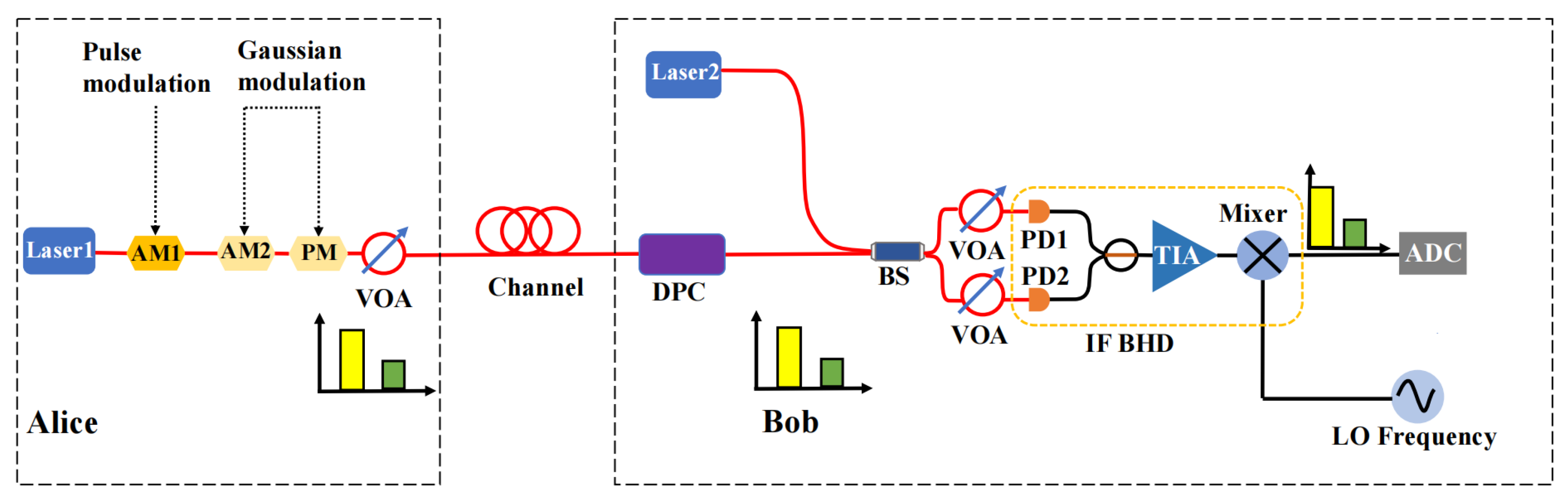
2. Local Local Oscillator CV-QKD Scheme

Here, the setup of the local local oscillator CV-QKD system with the intermediate-frequency BHD inspired by [33,34] will be introduced. We adopt the GMCS and heterodyne detection scheme where there exists a frequency difference between signal laser and local LO laser. The structure of the LLO CV-QKD scheme is shown in Figure 1. At Alice’s side, the continuous-wave laser (Laser1) at 1550.12 nm produces coherent light. Then, the light source is modulated by an amplitude modulator (AM1) at a repetition rate of f sym to generate pulse trains of width w sym , including signal pulses and time-multiplexed pilot pulses of higher optical power. To implement the overall Gaussian modulation, another phase modulator (PM) and amplitude modulator (AM2) utilize the electrical modulation signals generated by the digital-to-analog converter (DAC) to modulate the signal pulses, respectively, according to a uniform distribution and a Rayleigh distribution. Note that at this stage, the pilot pulses are further modulated to carry the information used for frequency offset and phase compensation. Then, a variable optical attenuator (VOA) is utilized to attenuate the signal pulses into a weak quantum signal with an optimal modulation variance V A and attenuate pilot pulses.
After transmitting over a quantum channel of optical fiber, they are received by the other legitimate user Bob. In the receiver, we use a dynamic polarization controller (DPC) to align the state of polarization (SOP) of the quantum signal, in order to maintain the optimal polarization state of the signal to improve the quality as high as possible. Then, the signal pulses interfere stably with the LO produced by the laser at 1550.12 nm (Laser2) through the 50:50 beam splitter (BS). Then, two VOAs after the output of BS are used for compensating the unbalance and symmetry of the BS in front of the intermediate-frequency BHD and then fed into the BHD. Note that the frequency offset between the laser at the sender and the laser at the receiver can be seen in the frequency spectrum, which is about 200 MHz in our experiment. Therefore, our self-developed 270 MHz intermediate-frequency BHD is suitable for our experiment system.
In the following, the output of the intermediate-frequency BHD will be derived [35]. For simplicity, we take the x quadrature as an example. First, the complex electric field of the quantum signal before entering into BS is represented by
E s ( t ) = A s ( t ) exp i ω s t + θ s ( t ) ,
where A s ( t ) and ω s are the amplitude and frequency of the signal field, respectively, θ s is the initial phase of the quantum signal. The complex electric field of the LO before entering into BS is similarly represented by
E LO ( t ) = A LO exp i ω LO t + θ LO ( t ) ,
where A LO and ω LO are the constant amplitude and frequency of the LO field, respectively, θ LO is the initial phase of the LO.
The balanced detection stage consists of a 50:50 beam splitter, a pair of PDs, and the subtractor, which suppress the direct current component and amplify the weak quantum signal by multiplying the strong LO. After interfering through the 50:50 BS, the electric fields injecting the PD1 and PD2 are derived as
E 1 = 1 2 E s + E LO , E 2 = 1 2 E s E LO ,
and the resultant photocurrents are therefore given by
I 1 ( t ) = k R Re A s ( t ) exp i ω s t + θ s ( t ) + A LO exp i ω LO t + θ LO ( t ) 2 ms = R 2 P s ( t ) + P LO + 2 P s ( t ) P LO cos ω I F t + θ s ( t ) θ LO ( t ) ,
I 2 ( t ) = k R Re A s ( t ) exp i ω s t + θ s ( t ) A LO exp i ω LO t + θ LO ( t ) 2 ms = R 2 P s ( t ) + P LO 2 P s ( t ) P LO cos ω I F t + θ s ( t ) θ LO ( t ) ,
where “Re” represents the real part, “ms” represents the mean of the square with respect to the optical frequencies, ω IF is the intermediate frequency from the frequency difference between signal and LO given by ω IF = ω s ω LO , R is the responsivity of PD, P s ( t ) and P LO are the optical power of the signal and LO. Thus, the output from the subtractor can be obtained
I ( I F ) = I 1 ( t ) I 2 ( t ) = 2 R P s ( t ) P LO × cos ω IF t + θ s ( t ) θ LO ( t ) .
We find from Equation (6) that the output photocurrent is proportional to P s . Furthermore, the intermediate-frequency BHD moves the intermediate-frequency output to the base band via a mixer and the intermediate-frequency LO, which gives:
I ( t ) = I 1 ( t ) I 2 ( t ) = R P s ( t ) P LO × cos θ s ( t ) θ LO ( t ) .

3. High-Performance Intermediate-Frequency BHD

In this section, the schematic diagram of intermediate-frequency BHD is introduced, which is mainly composed of a radio frequency-integrated circuit. Moreover, we design an optical test structure to prove the high performance of intermediate-frequency BHD in the telecommunication wavelength region.

3.1. Circuit Design

The simplified electronic circuit schematic of the intermediate-frequency BHD is shown in Figure 2, which is mainly composed of three parts. The first part is the photoelectric conversion section, which includes two reverse-biased InGaAs photodiodes (Hamamatsu, G9801-32, bandwidth: 2 GHz, junction capacitance: 1 pF, sensitivity ratio: 90% and quantum-efficiency: 72.2% at 1550 nm). The PDs generate the current signal, which is amplified by the circuit amplification part. The second part is the circuit amplification section, which consists of a resistor and a triple-stage ratio frequency (RF) amplification chip. First, the current signal is amplified by the ground resistance to achieve current-to-voltage conversion. Then a triple-stage RF amplification chip (ADI, ADL5523) is used to amplify the voltage signal. Traditional design prefers to use the trans-impedance amplification chip, and the trans-impedance amplifier (TIA) performs well in the low frequency, typically around tens of MHz. However, for intermediate-frequency BHD, the trans-impedance amplification chip cannot meet the requirements. Because of the limitation of the gain-bandwidth product (GBP), the gain of the amplifier decreases as the operating frequency increases. For the trans-impedance amplification chip, the value of the GBP is fixed, so the balance of the gain and operating bandwidth needs to be considered. The bandwidth of general TIA starts from DC to a variable frequency, and typically stops at tens of MHz. Moreover, the designed working frequency of the intermediate-frequency BHD is not in the base band, so the TIA chip is not the right choice.
To resolve this problem, we decided to use a more suitable RF amplification chip because it can meet the design requirements of the circuit amplification section. However, the RF amplification chip also has several disadvantages. Taking the ADL5523 RF amplification chip as an example, the gain and bandwidth of the chip are fixed, which causes difficulties in adjusting the amplifier’s circuit flexibly according to the design requirements. The purpose of the down-conversion section is to shift the intermediate-frequency signal to the base band, which is the last part. Considering the working frequency and the conversion loss, it is an excellent choice to use the frequency mixer chip (JMS) from Mini-Circuits. Moreover, we can not ignore the impedance mismatching of the frequency mixer, which has a significant influence on the bandwidth of the intermediate-frequency BHD, so it is quite essential to design the surrounding circuit of the frequency mixer.
The whole intermediate-frequency amplification circuit, apart from the RFIC, has an enormous impact on the performance of the circuit, considering the influence of the junction capacitance of PD and the parasitic capacitance of the PCB are also significant. To reduce the impact of these factors, we decide to select the Hamamatsu G9801-32 PD, which has excellent performance, and its junction capacitance of PD is only 0.5 pF. Meanwhile, we take some other measures (such as decreasing the length of the PD pins, optimizing the designed PCB structure, using a smaller package to make the structure more compact) to reduce the value of parasitic capacitance. Finally, the solder PCB is placed in an electromagnetic shielding box to minimize the electromagnetic radiation.
Figure 3 shows the diagram structure of the optical experiment. First, the laser generates a 1550 nm continuous-wave light, and a VOA1 is utilized to attenuate the signal power. The pulsed signal generated by an arbitrary waveform generator (AWG) is modulated into the continuous-wave light by an amplitude modulator. Then, the signal light interferes with the vacuum through the 50:50 BS after which the outputs are followed by a variable optical delay (VOD) and a VOA2 for keeping a perfect balance of two arms. The amplified intermediate-frequency signal is moved to the base band by a mixer, and a low pass filter (LPF) is utilized to filter out the useless signal. Finally, we use the spectrum analyzer (Rigal DSA815) and the oscilloscope (Keysight Technology MSOS804A) to analyze the output signal.

3.2. Bandwidth and QCNR

To prove the designed intermediate-frequency BHD can be applied in the local local oscillator CV-QKD, we have taken several relevant measurements on the frequency domain and time domain to obtain the information about QCNR, noise, and bandwidth. The test structure diagram can be obtained by removing the AM in Figure 3. The frequency mixer is indispensable for intermediate-frequency BHD, so the test results should include the measurement without the frequency mixer and the measurement with the frequency mixer. Figure 4a shows the bandwidth and noise power of the intermediate-frequency BHD without the frequency mixer. In this part, the bandwidth of the band pass area is from 300 MHz to 800 MHz. The output noise power of the amplification circuit starts to rise slowly from around kHz, reaching a high point at 300 MHz, and beginning to drop sharply from 800 MHz. Nevertheless, the downtrend from 900 MHz to 1200 MHz is not intuitive, and the main reason is that the frequency response design of the intermediate-frequency amplification circuit is not perfect. Although the intermediate-frequency amplification circuit has some defects, the whole performance of the circuit is excellent compared with other BHDs. Figure 4b shows the bandwidth and noise power of the intermediate-frequency BHD with the frequency mixer. The LO input of the mixer is a 500 MHz sine signal, which is necessary to obtain the down-conversion signal. Because the effect of low-frequency 1/f noise is eliminated, the quantum noise curve starts from DC rather than kHz. Simultaneously, the electronic noise of the intermediate-frequency BHD reaches a low level, which is quite crucial for the local local oscillator CV-QKD. For intermediate-frequency BHD, the bandwidth is about 270 MHz, and the amplification gain is quite flat. The quantum noise power rises with the increase of the input optical power and starts to fall from 270 MHz. We also obtain the QCNR information of the intermediate-frequency BHD in Figure 4b. As the optical power increases, the output noise ranges from DC to 270 MHz rises, then rolls down owing to the limitation of the bandwidth. The QCNR of the intermediate-frequency can attach 14.9 dB when the optical power is 9 mW. When the optical power reaches a certain threshold, the noise spectrum starts to increase. If the optical power is much higher than the threshold, the noise spectrum becomes the background noise spectrum of the spectrum analyzer. The main reason is that the amplification circuit has already saturated when the optical power exceeds the threshold.
The electronic and quantum noise in BHD are subject to Gaussian distribution. Meanwhile, the intermediate-frequency BHD is AC-coupled, so the mean of the noise is zero. In practice, the quantum noise variance cannot be measured in complete isolation from source of classical noise, so for intermediate-frequency BHD, the measured total noise variance of intermediate-frequency BHD by the oscilloscope is the sum of the quantum noise variance and the electronic noise variance. The electronic noise consists of the background noise of the instrument and electronic noise of intermediate-frequency BHD, which is mainly composed of the electronic noise of BHD. We obtain the electronic noise of intermediate-frequency BHD by the oscilloscope when the optical path is blocked, and the total noise is measured in different input optical powers. It is not difficult to obtain the corresponding quantum noise by subtracting the electronic noise from the total noise. We use the Keysight oscilloscope to measure the total noise and the electronic noise in the time domain. In order obtain enough data to analyze, we set the oscilloscope sampling rate to 10 GSa/s and set the time base to 1 μ s. First, we need to measure the electronic noise voltage when the optical power is zero under these test conditions. Then we can obtain the total noise voltage by changing the optical power. During the data processing, one data point is selected every 10 data points in the raw data to avoid correlation. It is vital to obtain the electronic noise and the total noise variance from the selected data. As shown in Figure 5a, it is clear that the quantum noise variance increases with the increase of the local oscillator power in an area, and we obtain the rough linear region of the intermediate-frequency BHD. The measured value of QCNR in the time domain is about 15 dB at a LO power of 9 mW. The limitations of measuring instruments cause the different values of the QCNR in the frequency domain and time domain. However, the QCNR in the time domain still has a perfect agreement with that in the frequency domain. After analyzing the above test results, it is evident that the idea of designing an intermediate-frequency BHD with high speed is achievable.

3.3. Linearity and Gain

In CV-QKD, random bits are encoded to the signal pulse at Alice’s side and recovered by the BHD at Bob’s side [36]. In order to minimize the measurement error, it is essential to guarantee that the intermediate-frequency BHD can work in a linear region. If the output of the intermediate-frequency BHD is not linearly dependent on the input, the measurement of the pulse quadrature will not be accurate. The performance of PD and the amplification chip both affect the linearity of the intermediate-frequency BHD. For PD, it has a linear region of photoelectric conversion. Simultaneously, the RF amplification chip also has a linear region to amplify the signal. So it is necessary to ensure that both the PD and the amplification circuit work in the linear region. We obtain the linearity test structure by making a small change to the structure in Figure 3. The optical test power should not be too large to ensure that the PD and amplifier can work in the linear region as well. The designed BHD works in the intermediate frequency, so an AWG is used to generate a sine wave with a frequency of 550 MHz, and the duty cycle is 50%. In the test, the pulsed light is sent to one photodiode of intermediate-frequency BHD when another photodiode is blocked. The amplitude of the output voltage is recorded by the oscilloscope and saves the corresponding optical power. Then, the same pulsed light is sent to another photodiode and measures the output voltage again. Figure 5b shows the output voltage of the two PDs at different optical power ranging from 3 μ W to 25 μ W. The trans-impedance gain of BHD is approximately equivalent to the slope of the line, which is about 22.4 k.

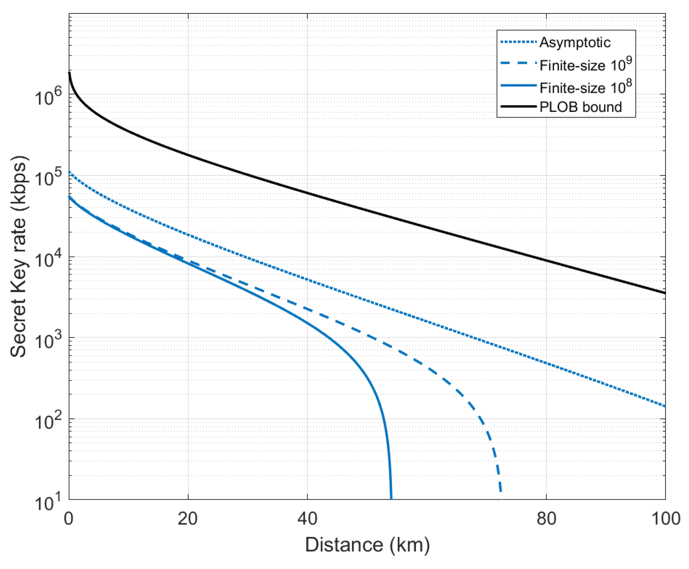
4. System Performance with Intermediate-Frequency BHD

Based on the above introduction about the performance of the intermediate-frequency BHD, the security analysis of Gaussian-modulated coherent states and heterodyne detection against collective attacks under an asymptotic scenario is given, and we make a simulation to evaluate the performance of local local oscillator CV-QKD system with the application of the designed intermediate-frequency BHD. As mentioned in Section 3, the measured electronic noise v el is 0.0384, the detection efficiency η is 0.612, and the bandwidth of the detector is 270 MHz. Combined with the variance of the EPR state [37] V = 4 = V A + 1 where V A is the modulation variance, channel transmittivity T = 10 α L / 10 where α = 0.2 dB/km is the loss coefficient of optical fiber, excess noise ε = 0.05 corresponding to a more general environment, we can evaluate the final secret key rate by using the following formula:
K = f sym ( β I AB χ BE ) ,
where β is the reconciliation efficiency in the post-processing stage, f sym is the aforementioned repetition rate, I AB is the mutual information between legitimate users Alice and Bob, and χ BE is the Holevo bound. I AB is represented by
I AB = log 2 V + χ tot 1 + χ tot ,
where χ tot is the total additional noise defined at the channel input, which can be calculated by χ tot = χ line + χ het / T , where χ line = ( 1 + T ε ) / T 1 = 1 / T 1 + ε represents the total channel-added noise defined at channel input, χ het = 1 + ( 1 η ) + 2 v el / η represents the total detector-added noise defined at channel input, and T is the channel transmittivity, in which ε is the excess noise, v el is the electric noise of the detector, η is the detection efficiency. As for the calculation of χ BE , it is as follows
χ BE = i = 1 2 G λ i 1 2 i = 3 5 G λ i 1 2
where G ( x ) = ( x + 1 ) log 2 ( x + 1 ) x log 2 x , λ i represent the symplectic eigenvalues of covariance matrices given by
λ 1 , 2 2 = 1 2 [ A ± A 2 4 B ] , λ 3 , 4 2 = 1 2 [ C ± C 2 4 D ] , λ 5 = 1 ,
where for heterodyne detection case
A = V 2 ( 1 2 T ) + 2 T + T 2 V + χ line 2 B = T 2 V χ line + 1 2 C = 1 T 2 V + χ tot 2 [ A χ het 2 + B + 1 + 2 χ het V B + T ( V + χ line ) + 2 T ( V 2 1 ) ] D = V + B χ het T ( V + χ tot ) 2
According to the above calculation, we make a simulation about the secret key rates as a function of distance of Gaussian-modulated coherent states and heterodyne detection against collective attacks. The simulation results of adopting such intermediate-frequency detectors in the local local oscillator CV-QKD scheme is shown in Figure 6. The blue solid curve, blue dot-dashed curve, and blue dotted curve correspond to the block lengths of N = 10 8 , N = 10 9 , and the asymptotic effect. The PLOB bounds that demonstrate the fundamental limit of repeaterless quantum communications are also drawn in the Figure 6. It can be seen that the secret key rate of the block length N = 10 8 reaches 1.506 Mbps at 40 km. When the block length is N = 10 9 , a key rate of 430.8 kbps can be achieved in our 60 km optical fiber transmission system. As can be seen from the above results, the designed intermediate-frequency BHD can help to obtain a high secret key rate, which is enough to support the metropolitan applications.

5. Conclusions

In this paper, we design a new intermediate-frequency balanced homodyne detector for local local oscillator continuous-variance quantum key distribution. For local local oscillator continuous-variance quantum key distribution system, the designed intermediate-frequency balanced homodyne detector can help reduce the complexity of the system, decrease the noise, and expand the capacity of the system. The bandwidth of the intermediate-frequency balanced homodyne detector is about 270 MHz, the quantum-to-classical noise ratio is around 14.9 dB and the trans-impedance gain is around 22.4 k. By adopting the intermediate-frequency BHD, the secret key rate of the pilot-sequential Gaussion-modulated coherent state (GMCS) CV-QKD system with a local local oscillator can reach over 430.8 kbps of 60 km. From the results, we can intuitively see the superior performance of the intermediate-frequency BHD.

Author Contributions

Conceptualization, D.Q., X.W. and Z.C.; methodology, D.Q.; formal analysis, D.Q. and X.W.; investigation, D.Q.; resources, X.W. and S.Y.; writing—original draft preparation, D.Q.; writing—review and editing, X.W., Z.C., Y.L. and S.Y.; visualization, Z.C.; supervision, X.W., Y.L. and S.Y.; project administration, X.W. and Z.C.; funding acquisition, X.W. and Z.C. All authors have read and agreed to the published version of the manuscript.

Funding

This work was supported by the National Natural Science Foundation of China under Grant No. 62001041, No. 62201012, the Fundamental Research Funds of BUPT under Grant No. 2022RC08, the Fund of State Key Laboratory of Information Photonics and Optical Communications under Grant No. IPOC2022ZT09, and Stability Program of Science and Technology on Communication Security Laboratory (2022).

Data Availability Statement

Not applicable.

Conflicts of Interest

The authors declare no conflict of interest.

References

  1. Pirandola, S.; Andersen, U.L.; Banchi, L.; Berta, M.; Bunandar, D.; Colbeck, R.; Englund, D.; Gehring, T.; Lupo, C.; Ottaviani, C.; et al. Advances in quantum cryptography. Adv. Opt. Photonics 2020, 12, 1012–1236. [Google Scholar] [CrossRef] [Green Version]
  2. Xu, F.; Ma, X.; Zhang, Q.; Lo, H.K.; Pan, J.W. Secure quantum key distribution with realistic devices. Rev. Mod. Phys. 2020, 92, 025002. [Google Scholar] [CrossRef]
  3. Bennet, C.H. Quantum cryptography: Public-key distribution and coin tossing. In Proceedings of the IEEE International Conference on Computers, Systems and Signal Processing, Bangalore, India, 9–12 December 1984; pp. 175–179. [Google Scholar]
  4. Grosshans, F.; Grangier, P. Continuous variable quantum cryptography using coherent states. Phys. Rev. Lett. 2002, 88, 057902. [Google Scholar] [CrossRef] [Green Version]
  5. Leverrier, A. Composable security proof for continuous-variable quantum key distribution with coherent states. Phys. Rev. Lett. 2015, 114, 070501. [Google Scholar] [CrossRef] [Green Version]
  6. Leverrier, A. Security of continuous-variable quantum key distribution via a Gaussian de Finetti reduction. Phys. Rev. Lett. 2017, 118, 200501. [Google Scholar] [CrossRef] [PubMed] [Green Version]
  7. Ghorai, S.; Grangier, P.; Diamanti, E.; Leverrier, A. Asymptotic security of continuous-variable quantum key distribution with a discrete modulation. Phys. Rev. X 2019, 9, 021059. [Google Scholar] [CrossRef] [Green Version]
  8. Lin, J.; Upadhyaya, T.; Lütkenhaus, N. Asymptotic security analysis of discrete-modulated continuous-variable quantum key distribution. Phys. Rev. X 2019, 9, 041064. [Google Scholar] [CrossRef] [Green Version]
  9. Pirandola, S. Composable security for continuous variable quantum key distribution: Trust levels and practical key rates in wired and wireless networks. Phys. Rev. Res. 2021, 3, 043014. [Google Scholar] [CrossRef]
  10. Denys, A.; Brown, P.; Leverrier, A. Explicit asymptotic secret key rate of continuous-variable quantum key distribution with an arbitrary modulation. Quantum 2021, 5, 540. [Google Scholar] [CrossRef]
  11. Wang, X.; Wang, H.; Zhou, C.; Chen, Z.; Yu, S.; Guo, H. Continuous-variable quantum key distribution with low-complexity information reconciliation. Opt. Express 2022, 30, 30455–30465. [Google Scholar] [CrossRef]
  12. Huang, L.; Wang, X.; Chen, Z.; Sun, Y.; Yu, S.; Guo, H. Countermeasure for Negative Impact of a Practical Source in Continuous-Variable Measurement-Device-Independent Quantum Key Distribution. Phys. Rev. Appl. 2023, 19, 014023. [Google Scholar] [CrossRef]
  13. Chen, Z.; Wang, X.; Yu, S.; Li, Z.; Guo, H. Continuous-mode quantum key distribution with digital signal processing. Npj Quantum Inf. 2023, 9, 28. [Google Scholar] [CrossRef]
  14. Wang, X.; Xu, M.; Zhao, Y.; Chen, Z.; Yu, S.; Guo, H. Non-Gaussian reconciliation for continuous-variable quantum key distribution. Phys. Rev. Appl. 2023, 19, 054084. [Google Scholar] [CrossRef]
  15. Jouguet, P.; Kunz-Jacques, S.; Leverrier, A.; Grangier, P.; Diamanti, E. Experimental demonstration of long-distance continuous-variable quantum key distribution. Nat. Photonics 2013, 7, 378–381. [Google Scholar] [CrossRef] [Green Version]
  16. Eriksson, T.A.; Hirano, T.; Puttnam, B.J.; Rademacher, G.; Luís, R.S.; Fujiwara, M.; Namiki, R.; Awaji, Y.; Takeoka, M.; Wada, N.; et al. Wavelength division multiplexing of continuous variable quantum key distribution and 18.3 Tbit/s data channels. Commun. Phys. 2019, 2, 9. [Google Scholar] [CrossRef] [Green Version]
  17. Tian, Y.; Wang, P.; Liu, J.; Du, S.; Liu, W.; Lu, Z.; Wang, X.; Li, Y. Experimental demonstration of continuous-variable measurement-device-independent quantum key distribution over optical fiber. Optica 2022, 9, 492–500. [Google Scholar] [CrossRef]
  18. Pan, Y.; Wang, H.; Shao, Y.; Pi, Y.; Li, Y.; Liu, B.; Huang, W.; Xu, B. Experimental demonstration of high-rate discrete-modulated continuous-variable quantum key distribution system. Opt. Lett. 2022, 47, 3307–3310. [Google Scholar] [CrossRef]
  19. Huang, Y.; Shen, T.; Wang, X.; Chen, Z.; Xu, B.; Yu, S.; Guo, H. Realizing a downstream-access network using continuous-variable quantum key distribution. Phys. Rev. Appl. 2021, 16, 064051. [Google Scholar] [CrossRef]
  20. Wang, X.; Chen, Z.; Li, Z.; Qi, D.; Yu, S.; Guo, H. Experimental upstream transmission of continuous variable quantum key distribution access network. Opt. Lett. 2023, 48, 3327–3330. [Google Scholar] [CrossRef]
  21. Ma, X.C.; Sun, S.H.; Jiang, M.S.; Liang, L.M. Local oscillator fluctuation opens a loophole for Eve in practical continuous-variable quantum-key-distribution systems. Phys. Rev. A 2013, 88, 022339. [Google Scholar] [CrossRef] [Green Version]
  22. Jouguet, P.; Kunz-Jacques, S.; Diamanti, E. Preventing calibration attacks on the local oscillator in continuous-variable quantum key distribution. Phys. Rev. A 2013, 87, 062313. [Google Scholar] [CrossRef] [Green Version]
  23. Zheng, Y.; Liu, W.; Cao, Z.; Peng, J. Monitoring scheme against local oscillator attacks for practical continuous-variable quantum-key-distribution systems in complex communication environments. Phys. Rev. A 2020, 101, 022319. [Google Scholar] [CrossRef]
  24. Qi, B.; Lougovski, P.; Pooser, R.; Grice, W.; Bobrek, M. Generating the local oscillator “locally” in continuous-variable quantum key distribution based on coherent detection. Phys. Rev. X 2015, 5, 041009. [Google Scholar] [CrossRef] [Green Version]
  25. Soh, D.B.; Brif, C.; Coles, P.J.; Lütkenhaus, N.; Camacho, R.M.; Urayama, J.; Sarovar, M. Self-referenced continuous-variable quantum key distribution protocol. Phys. Rev. X 2015, 5, 041010. [Google Scholar] [CrossRef] [Green Version]
  26. Huang, D.; Huang, P.; Lin, D.; Wang, C.; Zeng, G. High-speed continuous-variable quantum key distribution without sending a local oscillator. Opt. Lett. 2015, 40, 3695–3698. [Google Scholar] [CrossRef]
  27. Kleis, S.; Rueckmann, M.; Schaeffer, C.G. Continuous variable quantum key distribution with a real local oscillator using simultaneous pilot signals. Opt. Lett. 2017, 42, 1588–1591. [Google Scholar] [CrossRef]
  28. Marie, A.; Alléaume, R. Self-coherent phase reference sharing for continuous-variable quantum key distribution. Phys. Rev. A 2017, 95, 012316. [Google Scholar] [CrossRef] [Green Version]
  29. Wang, T.; Huang, P.; Zhou, Y.; Liu, W.; Zeng, G. Pilot-multiplexed continuous-variable quantum key distribution with a real local oscillator. Phys. Rev. A 2018, 97, 012310. [Google Scholar] [CrossRef]
  30. Laudenbach, F.; Schrenk, B.; Pacher, C.; Hentschel, M.; Fung, C.H.F.; Karinou, F.; Poppe, A.; Peev, M.; Hübel, H. Pilot-assisted intradyne reception for high-speed continuous-variable quantum key distribution with true local oscillator. Quantum 2019, 3, 193. [Google Scholar] [CrossRef] [Green Version]
  31. Shen, T.; Wang, X.; Chen, Z.; Tian, H.; Yu, S.; Guo, H. Experimental Demonstration of LLO Continuous-Variable Quantum Key Distribution With Polarization Loss Compensation. IEEE Photonics J. 2023, 15, 1–9. [Google Scholar] [CrossRef]
  32. Jin, X.; Su, J.; Zheng, Y.; Chen, C.; Wang, W.; Peng, K. Balanced homodyne detection with high common mode rejection ratio based on parameter compensation of two arbitrary photodiodes. Opt. Express 2015, 23, 23859–23866. [Google Scholar] [CrossRef] [PubMed] [Green Version]
  33. Comandar, L.C.; Brunner, H.H.; Bettelli, S.; Fung, F.; Karinou, F.; Hillerkuss, D.; Mikroulis, S.; Wang, D.; Kuschnerov, M.; Xie, C.; et al. A flexible continuous-variable QKD system using off-the-shelf components. In Quantum Information Science and Technology III; International Society for Optics and Photonics: Bellingham, WA, USA, 2017; Volume 10442, p. 104420A. [Google Scholar]
  34. Brunner, H.H.; Comandar, L.C.; Karinou, F.; Bettelli, S.; Hillerkuss, D.; Fung, F.; Wang, D.; Mikroulis, S.; Yi, Q.; Kuschnerov, M.; et al. A low-complexity heterodyne CV-QKD architecture. In Proceedings of the 2017 19th International Conference on Transparent Optical Networks (ICTON), Girona, Spain, 2–6 July 2017; pp. 1–4. [Google Scholar]
  35. Kikuchi, K. Fundamentals of coherent optical fiber communications. J. Light. Technol. 2015, 34, 157–179. [Google Scholar] [CrossRef]
  36. Chi, Y.M.; Qi, B.; Zhu, W.; Qian, L.; Lo, H.K.; Youn, S.H.; Lvovsky, A.; Tian, L. A balanced homodyne detector for high-rate Gaussian-modulated coherent-state quantum key distribution. New J. Phys. 2011, 13, 013003. [Google Scholar] [CrossRef] [Green Version]
  37. Einstein, A.; Podolsky, B.; Rosen, N. Can quantum-mechanical description of physical reality be considered complete? Phys. Rev. 1935, 47, 777. [Google Scholar] [CrossRef] [Green Version]
  38. Pirandola, S.; Laurenza, R.; Ottaviani, C.; Banchi, L. Fundamental limits of repeaterless quantum communications. Nat. Commun. 2017, 8, 15043. [Google Scholar] [CrossRef] [PubMed] [Green Version]
  39. Pirandola, S.; Braunstein, S.L.; Laurenza, R.; Ottaviani, C.; Cope, T.P.; Spedalieri, G.; Banchi, L. Theory of channel simulation and bounds for private communication. Quantum Sci. Technol. 2018, 3, 035009. [Google Scholar] [CrossRef] [Green Version]
Figure 1. Diagram of the simplified local local oscillator CV-QKD architecture. AM: amplitude modulator, PM: phase modulator, BS: beam splitter, VOA: variable optical attenuator, DPC: dynamic polarization controller, PD: photodiode, TIA: trans-impedance amplifier, LO frequency: the local oscillator frequency of the mixer, ADC: analog-to-digital converter.
Symmetry 15 01314 g001
Figure 2. Simplified electronic circuit schematic of the intermediate-frequency BHD. V+: positive supply voltage, V-: negative supply voltage, PD: photodiode, ADL5523: ratio frequency amplification chip, JMS: frequency mixer chip, LPF: low-pass filter.
Symmetry 15 01314 g002
Figure 3. Diagram of the optical experiment. The red lines are optical paths, and the black lines are electrical paths. Laser: 1550 nm continuous-wave fiber laser, AWG: arbitrary waveform generator, VOA: variable optical attenuators, VOD: variable optical delay, AM: amplitude modulator, BS: beam splitter, PD: photodiode, LO: local oscillator, LPF: low pass filter.
Symmetry 15 01314 g003
Figure 4. (a) Measured noise power of intermediate-frequency BHD without a mixer ranging from kHz to 1.5 GHz. BHD noise spectrum at CW LO powers of 0.5, 1, 2, 3, 4, 5, 7, 9 mW (from the third lowest to highest curve). Bg noise: Spectrum analyzer background noise spectrum, Ele noise: BHD electronic noise spectrum, resolution bandwidth: 100 kHz. (b) Measured noise power of intermediate-frequency BHD with mixer and LPF. Intermediate-frequency BHD noise spectrum at CW LO powers of 0.5, 1, 2, 3, 4, 5, 7, 9 mW (from the third lowest to highest curve). LPF: DC-270 MHz. Resolution bandwidth: 100 kHz.
Symmetry 15 01314 g004
Figure 5. (a) Noise variance as a function of the CW LO power in the time domain. The red curve is the total noise composed of electronic noise and quantum noise. The black line is electronic noise from the BHD and other instruments. The green curve is quantum noise obtained by subtracting the electronic noise from the total noise. The quantum noise variance to the electronic noise variance ratio is 15.0 dB at a LO power of 9 mW. (b) Intermediate-frequency BHD output voltage as a function of the optical power. The “PD+” and “PD−” are reversely biased photodiodes to generate the opposite current. The black squares are the output voltage when only “PD+” is illuminated, and the red triangles are the output voltages when only “PD−” is illuminated. The black line represents the fitting line of the output voltage.
Symmetry 15 01314 g005
Figure 6. Secure key rate as a function of the transmission distance-based intermediate-frequency BHD. The blue curves from left to right represent the achievable key rate considering the finite-size effect with N = 10 8 , N = 10 9 , and the asymptotic effect. Besides, the black curve corresponds to the PLOB bound [38,39]. Other parameters in our results are as follows: the modulation variance V A = 3 , the electronic noise v e l = 0.0384 , the detection efficiency η = 0.612 , the loss coefficient of optical fiber α = 0.2 dB/km, and the excess noise ε = 0.05 .
Symmetry 15 01314 g006
Disclaimer/Publisher’s Note: The statements, opinions and data contained in all publications are solely those of the individual author(s) and contributor(s) and not of MDPI and/or the editor(s). MDPI and/or the editor(s) disclaim responsibility for any injury to people or property resulting from any ideas, methods, instructions or products referred to in the content.

