Article

Analysis of a Heterogeneous Queuing Model with Intermittently Obtainable Servers under a Hybrid Vacation Schedule

by
Divya Kothandaraman
and
Indhira Kandaiyan
*
Department of Mathematics, School of Advanced Sciences, Vellore Institute of Technology, Vellore 632 014, Tamil Nadu, India
*
Author to whom correspondence should be addressed.
Symmetry 2023, 15(7), 1304; https://doi.org/10.3390/sym15071304
Submission received: 2 November 2022 / Revised: 22 December 2022 / Accepted: 24 December 2022 / Published: 24 June 2023
(This article belongs to the Special Issue Mathematical Models: Methods and Applications)

Abstract

:
This paper investigates the concept of a Markovian queueing model with heterogeneous, intermittently available servers with feedback under a hybrid vacation policy. Both the asymmetric transition representation and the hybrid vacation policy are addressed in this article. The necessary and sufficient conditions for system stability are presented. In addition, the steady-state probability distribution of the queueing model was derived by employing the matrix geometric method. Furthermore, a few formulae were constructed to determine the model’s performance indicators. Finally, the influence of system parameters was also investigated using some numerical examples.

1. Introduction

The queuing theory focuses on understanding the varied dynamics of lines, or “queues,” and how to improve their effectiveness. The queueing theory and related models are used to represent real-world queueing situations so that the queueing performance may be mathematically investigated. It makes use of the origin, planning capacity, performance evaluation, statistics, and energetic optimization of numerous actual things and processes, and is a useful tool for simulating production lines, operating systems, communication and transportation networks, etc. Generally speaking, homogenous servers are the focus of current research on multi-server queueing methods; that is, each server’s individual service rates are the same. This assumption may be possible only if the servicing mechanism is mechanically or electronically managed. However, the presumption made above regarding this queueing scheme with humanistic servers is wildly unrealistic. When providing the same service, servers frequently serve at different rates. Numerous researchers were inspired by this to investigate the multi-server queueing approach with heterogeneous servers. Here, we analyzed a heterogeneous queueing model with an intermittently obtainable server under a hybrid vacation policy by incorporating the matrix geometric method.
The following is a summary of the remaining sections of this paper: The model’s construction and the quasi-birth–death process are presented in Section 2. In Section 3, the matrix geometric solution and the computation of steady-state probabilities are established. Section 4 presents several performance measures of the model and their practical applications. Section 5 discusses numerical examples of the paradigm under consideration. Section 6 contains a few graphical visualizations as well as its numerical findings. The final section contains the model’s concluding observations as well as its future scope.

Survey of Literature

In the heterogeneous queueing model, the servers provide service at a different rate. Morse [1] was the first to establish the theory of heterogeneity in service. Vijendra Singh [2] investigated the first Markovian queueing system with balking and two heterogeneous servers. Krishnamoorthy et al. [3] scrutinized a two-server Markovian queueing system with heterogeneous servers, including one that had a working vacation. Indra and Vijay Rajan [4] utilized the matrix geometric approach to analyze a Markovian queue with two heterogeneous servers and disasters. Leemans [5] explored the queue length distribution of a Markovian two-class, two-server queue, and he subsequently provided a method for calculating the waiting time distribution. A queueing model based on k sequential heterogeneous service steps and vacations was recently proposed by Mohammadi and Salehi rad [6]. Seenivasan et al. [7] studied a two-heterogeneous-server queueing model with an intermittently obtainable server by using the matrix geometric method.
Agarwal [8] first proposed the idea of an intermittently obtainable server where server 1 is readily available whereas server 2 is intermittently available; that is, server 2 performs a variety of strange and unusual tasks. Here, service interruptions happen for an arbitrary amount of time, but they occur only when the task at hand is finished. Such service is described as an intermittently obtainable service. Sharda [9] addressed a queuing problem with an intermittently available server with entries and exits in batches of varying sizes. Seenivasan et al. [10] recently investigated a heterogeneous queueing system with an intermittently available server with failures and restoration.
In recent years, queueing systems with vacations have gained popularity. Server vacations might occur as a result of a server outage, or the assignment of another duty to the server. Levy and Yechiali [11] were the first to explore the idea of a vacation and to calculate the optimum length of a vacation using the decomposition result. The review papers by Doshi [12] and Takagi [13] highlight the growing amount of research being conducted on queueing systems with vacations. There has been a recent trend in vacation queues that refers to “working vacation”, which is when service is provided during vacation periods at a lower rate than usual; that is, while on vacation, the server continues to provide service but at a slower rate rather than stopping completely. Such a working vacation model was initially proposed by Servi and Finn [14]. Tian et al. [15] analyzed the M / M / 1 queue with a single working vacation. A recent assessment conducted by Ke et al. [16] summarized the most recent research findings on vacation and working vacation queueing systems over the last decade. A Markovian queueing model of an unreliable multi-station machine with a working vacation policy and impatient customers was investigated by Bouchentouf et al. [17]. Micheal Mathavavisakan and Indhira [18] recently analyzed an M / G / 1 retrial queueing model under working vacation and feedback for impatient customers. Zhang and Xu [19] researched an M / M / 1 queue with various working vacation periods and an N-policy. Mytalas and Zazanis [20] investigated a Markovian single-server queueing system with batch Poisson arrivals and instantaneous Bernoulli feedback that operated under a multiple-vacation policy.
The matrix geometric approach is a technique for analyzing continuous-time Markov chains with quasi-birth–death (Qbd) processes that include transition rate matrices with repeating block structures. It is a helpful tool for dealing with the more complicated Markovian queueing problems. The matrix-geometric method in stochastic models was first proposed by Neuts [21]. Xu et al. [22] designed an M / M / 1 queue with a single working vacation using the QBD process and the matrix-geometric solution approach. Vijayashree and Janani [23] studied the transient nature of a queueing model with differentiated vacations. Shekhar et al. [24] employed a matrix-geometric method to determine the queue-size distribution for the queueing model with a Bernoulli scheduled vacation and maintenance of the reneging customer. Roshli Aniyeri and Ratnam [25] recently studied an M / M / 2 queueing system with multi-servers without a vacation by utilizing the matrix geometric method.
The majority of studies on queueing theory describe queueing systems where the service stations are reliable; that is, they do not fail. However, in fact, we often come across situations where a service station could break down but might be repaired. There are several sectors where server failure events might happen, including computers, communication networks, flexible manufacturing systems, the automotive industry, etc. The queueing system with service interruptions was studied by Federgrune and Green [26]. A single-server working vacation queueing model with multiple types of server breakdowns was investigated by Madhu Jain et al. [27]. Kalyanaraman and Seenivasan [28] analyzed a multi-server retrial queue with breakdown and geometric loss. Renisagaya et al [29] studied the N-policy multiple-vacations queueing model with server breakdown and repair.
After obtaining a service, a dissatisfied or unhappy consumer may opt to try another one, which is known as “feedback ”, or they might decide to quit the system permanently after receiving quality service. Ayyappan et al. [30] conducted a study on single-server Markovian retrial queues with pre-emptive priority service and feedback. A single-server Markovian feedback queuing model with discouraged arrivals, reneging, and retention of reneging consumers with restricted capacity was examined by Sharma et al. [31].
A hybrid vacation is a blend of a working vacation (WV) and a complete vacation (CV), in which the server may initially move to WV and continue to give service but at a reduced rate while the system is inactive. If the system gets empty during WV, the server will switch to CV mode. However, if there are customers in WV, the server will stay in WV and provide services to those customers. If the customers are ready after the CV has been executed, the server will revert to its regular busy state and begin serving them. The research by Anshul Kumar et al. [32] focused on a two-stage service procedure with a hybrid vacation policy based on the matrix geometric technique.
Though many studies have been conducted in matrix geometric technique under various vacation policies, no one has conducted research on the matrix geometric technique in a heterogeneous queueing system with a hybrid vacation schedule. To address this need, this research paper investigated the effectiveness of the heterogeneous queueing model that is intermittently available under a hybrid vacation. Here, the hybrid vacation concept was extended to dual servers with different service rates where one server is always available, and the other one is intermittently obtainable.

2. Construction of the Model

Under the hybrid vacation policy, we propose an unreliable, heterogeneous, and intermittently available server with feedback. Our model is explained in the following way:
  • The arrival process: The arrival of the customer takes place according to a Poisson process with rate λ . Customers join the system in accordance with the availability of the server: server 1 is always available, whereas server 2 is only accessible in certain states, namely working vacation (WV), complete vacation (CV), intermittently attainable (IO), working (Wk), and breakdown (Bd).
  • The service process: Two distinct servers provide the service at two different rates under the first-in-first-out policy. In our model, server 1 is always accessible whereas server 2 is either working or under WV, CV, IO, or Bd. Moreover, server 2 starts performing certain critical and unusual tasks when the line length seems to be larger than or equal to zero. Server 2 must finish the current job before performing any unusual tasks. Servers 1 and 2 have service rates of μ 1 and μ 2 , respectively, and they follow an exponential distribution.
  • Vacation process: During the vacation time, server 2 automatically commences WV, which has an exponential distribution, with the slower service rate μ v . When server 2 gets empty during WV, the server will switch to CV mode. After the CV has been executed, the server will revert to its regular busy state and begin serving customers. The CV duration has an exponential distribution with a mean θ v . The retrieval capacity time on server 2 follows an exponential distribution with a rate of ξ . Server 2 enters the working period in the CV state with the probability ζ 0 to provide service to the customer, which is always 1.
  • Feedback rule: After obtaining a service, an unsatisfied customer can opt to enter for another service with probability ν ¯ , referred to as “feedback,” or they can choose to permanently leave the system with probability ν (=1− ν ¯ ).
  • Breakdown and repair policy: Server 2 may experience a breakdown, and therefore it is sent for repair immediately. In the meantime, the server stops serving consumers and waits for the repair to be completed. The breakdown rate of server 2 is γ and the repair rate is σ .
All stochastic processes in the system are independent of one another. The structure of the model’s transition diagram is depicted in the below Figure 1. Since transitions between all of the state spaces are conceivable in our paradigm, the transition description is asymmetrical.

Qbd Process

Let ϑ ( t ) = { ( S ( t ) , N ( t ) ) ; t 0 } be a Markov process (MP) with a state space at time t, where N ( t ) represents the no. of customers in the system, and
S ( t ) = 0 , if   server   2   is   in   Working   vacation 1 , if   server   2   is   in   Complete   vacation 2 , if   server   2   is   in   Intermittently   obtainable 3 , if   server   2   is   in   Working 4 , if   server   2   is   in   Breakdown
The system state is symbolized by S ( t ) and N ( t ) . Let { ( S ( t ) , ( N ( t ) ) ; t 0 } , and the state space be organized in lexicographical manner as follows:
Ω = { ( 0 , 0 ) ( 1 , 0 ) ( j , i ) | i 1 , j = 0 , 1 , 2 , 3 , 4 }
The infinitesimal generator matrix H is expressed as follows:
H = A 00 B 00 0 0 0 0 0 C 00 D 11 D 00 0 0 0 0 0 D 22 D 11 D 00 0 0 0 0 0 D 22 D 11 D 00 0 0 0 0 0 D 22 D 11 D 00 0
where
A 00 = ( λ + θ v ) θ v 0 λ ; B 00 = λ 0 0 0 0 0 λ 0 0 0 ; D 00 = λ 0 0 0 0 0 λ 0 0 0 0 0 λ 0 0 0 0 0 λ 0 0 0 0 0 λ
C 00 = ν ( μ 1 + μ v ) 0 0 0 ν μ 1 0 ν ( μ 1 + μ 2 ) 0 0 0 ; D 22 = ν ( μ 1 + μ v ) 0 0 0 0 0 0 0 0 0 0 0 ν μ 1 0 0 0 0 0 ν ( μ 1 + μ 2 ) 0 0 0 0 0 0 and
D 11 = ( λ + ν ( μ 1 + μ v ) ) 0 0 0 0 0 ( λ + ζ 0 ) 0 ζ 0 0 0 0 ( λ + ξ + ν μ 1 ) ξ 0 0 0 0 ( λ + γ + ν ( μ 1 + μ 2 ) ) γ 0 0 0 σ ( λ + σ )

3. Matrix Geometric Solution

     We define P j i = { ( S ( t ) = j , N ( t ) = i ) } , where j reflects the server state and i indicates the total number of customers in the queue. Under the stability condition ρ < 1 , the prob. vector is described as follows: G = [ G 0 , G 1 , G 2 , ] ,
where G 0 = [ g 0 , 0 , g 1 , 0 ] , i = 0 ;
    G 1 = [ g 0 , 1 , g 1 , 1 , g 2 , 1 , g 3 , 1 , g 4 , 1 ] ;
    G 2 = [ g 0 , 2 , g 1 , 2 , g 2 , 2 , g 3 , 2 , g 4 , 2 ] …, etc.
Here, we generalize G i = [ g 0 , i , g 1 , i , g 2 , i , g 3 , i , g 4 , i ] , i = 1 , 2 , 3 , 4 , .
The governing system of difference equations are obtained from the condition G H = 0 as follows:
G 0 A 00 + G 1 C 00 + 0 + = 0
G 0 B 00 + G 1 D 11 + G 2 D 22 + 0 + = 0
G 1 D 00 + G 2 D 11 + G 3 D 22 + 0 + = 0
G 2 D 00 + G 3 D 11 + G 4 D 22 + 0 + = 0
G i D 00 + G i + 1 D 11 + G i + 2 D 22 + = 0 where i 1
G k = G 1 R k 1 , where k 2 .
Let the matrix R represent the rate matrix. By substituting Equation ( 6 ) into Equations ( 1 ) ( 5 ) , we obtain
G 0 A 00 + G 1 C 00 = 0
G 0 B 00 + G 1 [ D 11 + R D 22 ] = 0
G 1 [ D 00 + R D 11 + R 2 D 22 ] = 0
G 1 R [ D 00 + R D 11 + R 2 D 22 ] = 0
G 1 R i 1 [ D 00 + R D 11 + R 2 D 22 ] = 0 , where i 2 .
The normalizing equation is given by
G 0 e + G 1 [ I R ] 1 e = 1
Here, e is a column vector in which all elements are 1s in the corresponding column. By using methodologies from Neuts [21] and Latouche and Ramaswami [33], we have estimated the rate matrix R.
Thus, R is a minimal non-negative solution of the matrix quadratic equations.
D 00 + D 11 R + D 22 R 2 = 0
R = D 00 D 11 1 R 2 D 22 D 11 1
where R≥ 0, and it is an irreducible non-negative matrix of a radius smaller than one (see [21] pp. 82–83).
Matrix R can be calculated using an iterative approach as shown below.
R 0 = 0
R k + 1 = D 00 D 11 1 R k 2 D 22 D 11 1 k 0
All values of R will expand monotonically. Here, the steady state is attained with the aid of the MGM.
G D 00 e < G D 22 e
Here, we derive the conditions for the ergodicity of the Markov process. Define D= D 00 + D 11 + D 22 , so D is given below:
D = 0 0 0 0 0 0 ζ 0 0 ζ 0 0 0 0 ξ ξ 0 0 0 0 γ γ 0 0 0 σ σ .
Matrix D is an irreducible and a least generator in a Markov process. Let us assume that G = [ G 0 , G 1 , G 2 , G 3 , G 4 ] is the stat. probability vector of the matrix D that satisfies the following condition [21]:
G D = 0 ; G e = 1
From Equation ( 19 ) , we obtain
G 0 = σ γ 2 + γ σ + σ ;
G 1 = 0 ;
G 2 = 0 ;
G 3 = γ σ γ 2 + γ σ + σ ;
G 4 = γ 2 γ 2 + γ σ + σ ;
Using Theorem 3.1.1 from Neuts [21], the necessary and sufficient condition for the stability of the system is obtained as follows: if we apply the stability condition ( 17 ) for QBD procedure in matrix G, we obtain
λ [ G 0 + G 1 + G 2 + G 3 + G 4 ] < ν μ 1 [ G 0 + G 2 + G 3 ] + ν μ v G 0 + ν μ 2 G 3
λ ( γ 2 + γ σ + σ ) < σ ν ( μ 1 + μ v ) + γ σ ν ( μ 1 + μ 2 ) .

3.1. The Rate Matrix and Steady-State Probability Computation

Let the stationary probability vector G = [ G 0 , G 1 , G 2 , ] be the unique solution. We apply the MGM to calculate the stationary probability vector. To achieve this, we must first identify the rate matrix R, which is the minimal non-negative solution for the matrix quadratic Equation ( 13 ) .
The rate matrix R can be evaluated by methods from Neuts [21] and Latouche and Ramaswami [33]. After that, under the stability state, we solve G H = 0 with the normalization condition Equation ( 12 ) . The algorithm for computing the rate matrix R and algorithm for calculating the steady-state probability vectors are summarized in the following.

3.2. Special Cases

Case(i): No complete vacation, no feedback
Let θ v = 0 and ν = 0 . Our model is reduced to a heterogeneous queueing model with an unreliable server and working vacation, which is similar to [34].
Case (ii): No working vacation, no complete vacation, no feedback, and no breakdown.
Let μ v = 0 , θ v = 0 , ν = 0 , and γ = 0 . Our model is reduced to a two-heterogeneous-server queuing model with an intermittently obtainable server, which coincides with [7].

4. Performance Indicators

     The following are some performance measurements for the queueing model under consideration in terms of steady-state probability.

4.1. Calculation of Steady-State Probabilities

  • Probability that the servers are idle: P S I d = g 0 , 0 ;
  • Probability that server 2 is in working vacation period P S 2 W v = i = 0 g 0 , i ;
  • Probability that server 2 is in complete vacation period P S 2 C v = i = 0 g 1 , i ;
  • Probability that server 2 is intermittently obtainable P S 2 I o = i = 1 g 2 , i ;
  • Probability that server 2 is in regular busy period P S 2 W k = i = 1 g 3 , i ;
  • Probability that server 2 is in breakdown period P S 2 B d = i = 1 g 4 , i .

4.2. Calculation of the Mean Number of Customers in the System

Mean system length:
  • When server 2 is on working vacation E N 1 = i = 1 i g 0 , i ;
  • When server 2 is on complete vacation E N 2 = i = 1 i g 1 , i ;
  • When server 2 is intermittently obtainable E N 3 = i = 1 i g 2 , i ;
  • When server 2 is in regular busy period E N 4 = i = 1 i g 3 , i ;
  • When server 2 is in breakdown period E N 5 = i = 1 i g 4 , i ;
  • Mean no. of customers present in the system L s = E N 1 + E N 2 + E N 3 + E N 4 + E N 5 .

4.3. Calculation of the Mean Number of Customers in the Queue

Mean queue length:
  • When server 2 is on working vacation E N q 1 = i = 1 ( i 1 ) g 0 , i ;
  • When server 2 is on complete vacation E N q 2 = i = 1 ( i 1 ) g 1 , i ;
  • When server 2 is intermittently obtainable E N q 3 = i = 1 ( i 1 ) g 2 , i ;
  • When server 2 is in regular busy period E N q 4 = i = 1 ( i 1 ) g 3 , i ;
  • When server 2 is in breakdown period E N q 5 = i = 1 ( i 1 ) g 4 , i ;
  • Mean no. of customers present in the queue L q = E N q 1 + E N q 2 + E N q 3 + E N q 4 + E N q 5 .

4.4. Practical Application of the Model

     The model’s real-world scenario may be presented using the example of a vehicle service station, where there are two servers providing distinct services. If a customer finds the service terminal, they will be welcomed by a service engineer, who will first provide the customer with the first service (server 1), such as checking minor faults in the vehicle, and then the second service engineer (chief engineer, server 2) will provide the second service, i.e., the major service. After receiving service from the engineer, the repaired vehicle will be returned to the customer. Server 1 is always accessible for checking minor faults, but server 2 may experience interruptions due to sporadic availability, breakdowns, or vacation.
If server 2 chooses to perform some other unusual jobs other than the original service, the customer has to complete their hand service, and if there are no major repair jobs at the service center, the chief engineer will undergo WV and work on a secondary assignment at a slower service rate. The engineer will take a CV when the WV is completed. If there are no repair jobs just after the completion of the CV, the chief engineer will remain in the CV state until at least one defective vehicle joins for repair work; in such a circumstance, it returns from the CV state to its regular busy state. It should be taken into account that, when server 1 is always busy, breakdowns in server 2 may occur, requiring general maintenance to execute its assigned tasks. Then, the damaged server 2 will be promptly repaired. Arrivals of defective vehicles for repair jobs in the system are not authorized while server 2 is being repaired. After gaining service, if the customers are unsatisfied (feedback), they will return back to the service terminal as a new arrival or they will leave the service station as satisfied customers. Therefore, the proposed model is highly useful for dealing with real-world queuing situations such as these.

5. Numerical Illustrations

In this part, we will illustrate the various parameters of the system behaviour measurements using MATLAB. We investigated service times and slower service times, both of which are exponentially distributed. The numerical measurements were chosen at random to meet the stability condition. The table below displays the estimated values for several features of our model, including the probability that the servers are idle ( P S I d ), the probability that server 2 is in a working vacation period ( P S 2 W v ), intermittently obtainable ( P S 2 I o ), regular busy period ( P S 2 W k ), or breakdown period ( P S 2 B d ), the average system size ( L s ), and the average queue size ( L q ).

5.1. Calculation of Rate Matrix R

In this section, we provide numerical examples to learn more about and understand the implementation of the λ , μ 1 , μ 2 , ν parameters in the system’s particular probabilistic representation features.

5.1.1. With Different Arrival Rate ( λ )

     The value of λ now varies whereas the remaining variables remain constant. First, the rate matrix was computed by using Algorithm 1. The rate matrix R was applied to Equations ( 1 ) ( 3 ) and solved to find the probability vectors G 0 and G 1 . Then, by substituting G 1 into Equation ( 6 ) , we can obtain the remaining vectors G i s (by Algorithm 2). Finally, we calculated the sum of the five components (i.e., G 0 , G 1 , G 2 , G 3 , and G 4 ) and confirmed that the aggregate probability value is approximately 1, as shown in Table 1.
Algorithm 1 An algorithm for computing rate matrix.
INPUT: D 00 , D 11 , D 22 , e is a column vector of 1s and ϵ
OUTPUT: R
Step 1: Set R 0 = 0 .
Step 2: while | ( D 00 + R ( k ) D 11 + R ( k ) 2 D 22 ) e ) | ϵ    k = 0, 1,...
    perform steps 3 and 4
Step 3: Set R ( k + 1 ) = D 00 D 11 1 R ( k ) 2 D 22 D 11 1 .    k = 0, 1...
Step 4: Continue Step 3 untill R ( k + 1 ) is close to R ( n ) .
Step 5: set R = R ( k + 1 )
Step 6: OUTPUT
Algorithm 2 An algorithm for steady-state probability vectors/
INPUT: A 00 , B 00 , D 00 , D 11 , D 22 , R, I, e 0 ,e is a column vector of 1s
OUTPUT: G 0 , G 1 , G 2 , G 3 ,
Step 1: A ← G 0 G 1 A 00 B 00 C 00 D 11 + R D 22
Step 2: Solve A=0
Step 3: B ← G 0 e 0 + G 1 ( I R ) 1 e
Step 4: Solve B=1
Step 5: G 0 , G 1 ← Solve (A,B)
Step 6: Compute the steady-state probability vectors
If k 2 compute G k = G 1 R k 1
Step 7: OUTPUT
Illustration 1: Assume that λ = 0.05 , μ 1 = 1.5 , μ 2 = 1 , μ v = 0.5 , ν = 0.7 , ν ¯ = 0.3 , ζ 0 = 1 , γ = 0.25 , σ = 1 , θ v = 0.1 , ξ = 0.5 and
R = 0.0357 0 0 0 0 0 0.0476 0 0.0323 0.0063 0 0 0.0319 0.0099 0.0021 0 0 0 0.0292 0.0066 0 0 0 0.0323 0.0539
Illustration 2: Assume that λ = 0.1 , μ 1 = 1.5 , μ 2 = 1 , μ v = 0.5 . ν = 0.7 , ν ¯ = 0.3 , ζ 0 = 1 , γ = 0.25 , σ = 1 , θ v = 0.1 , ξ = 0.5 and
R = 0.0714 0 0 0 0 0 0.0909 0 0.0737 0.0110 0 0 0.0631 0.0213 0.0037 0 0 0 0.0602 0.0121 0 0 0 0.0737 0.1019
Illustration 3: Assume that λ = 0.15 , μ 1 = 1.5 , μ 2 = 1 , μ v = 0.5 , ν = 0.7 , ν ¯ = 0.3 , ζ 0 = 1 , γ = 0.25 , σ = 1 , θ v = 0.1 , ξ = 0.5 and
R = 0.1071 0 0 0 0 0 0.1304 0 0.1276 0.0147 0 0 0.0937 0.0349 0.0050 0 0 0 0.0935 0.0169 0 0 0 0.1276 0.1451
Illustration 4: Assume that λ = 0.2 , μ 1 = 1.5 , μ 2 = 1 , μ v = 0.5 , ν = 0.7 , ν ¯ = 0.3 , ζ 0 = 1 , γ = 0.25 , σ = 1 , θ v = 0.1 , ξ = 0.5 and
R = 0.1429 0 0 0 0 0 0.1667 0 0.2015 0.0174 0 0 0.1234 0.0517 0.0060 0 0 0 0.1308 0.0209 0 0 0 0.2015 0.1841
Illustration 5: Assume that λ = 0.25 , μ 1 = 1.5 , μ 2 = 1 , μ v = 0.5 , ν = 0.7 , ν ¯ = 0.3 , ζ 0 = 1 , γ = 0.25 , σ = 1 , θ v = 0.1 , ξ = 0.5 and
R = 0.1768 0 0 0 0 0 0.2000 0 0.3174 0.0195 0 0 0.1524 0.0752 0.0068 0 0 0 0.1767 0.0244 0 0 0 0.3174 0.2195

5.1.2. With Different Service Rate ( μ 1 ) of Server 1

The value of μ 1 now varies, whereas the remaining variables remain constant. First, the rate matrix was computed by using Algorithm 1. The rate matrix R was applied to Equations ( 1 ) ( 3 ) and solved to find the probability vectors G 0 and G 1 . Then, by substituting G 1 into Equation ( 6 ) , we can obtain the remaining vectors G i s (by Algorithm 2). Finally, we calculated the sum of the five components (i.e., G 0 , G 1 , G 2 , G 3 , and G 4 ) and confirmed that the aggregate probability value is approximately 1, as shown in Table 2.
Illustration 1: Assume that λ = 0.1 , μ 1 = 2 , μ 2 = 1 , μ v = 0.5 , ν = 0.7 , ν ¯ = 0.3 , ζ 0 = 1 , γ = 0.25 , σ = 1 , θ v = 0.1 , ξ = 0.5 and
R = 0.0571 0 0 0 0 0 0.0909 0 0.0638 0.0093 0 0 0.0519 0.0142 0.0026 0 0 0 0.0500 0.0102 0 0 0 0.0638 0.1002
Illustration 2: Assume that λ = 0.1 , μ 1 = 2.5 , μ 2 = 1 , μ v = 0.5 , ν = 0.7 , ν ¯ = 0.3 , ζ 0 = 1 , γ = 0.25 , σ = 1 , θ v = 0.1 , ξ = 0.5 and
R = 0.0476 0 0 0 0 0 0.0909 0 0.0569 0.0080 0 0 0.0440 0.0101 0.0019 0 0 0 0.0428 0.0088 0 0 0 0.0569 0.0989
Illustration 3: Assume that λ = 0.1 , μ 1 = 3 , μ 2 = 1 , μ v = 0.5 , ν = 0.7 , ν ¯ = 0.3 , ζ 0 = 1 , γ = 0.25 , σ = 1 , θ v = 0.1 , ξ = 0.5 and
R = 0.0408 0 0 0 0 0 0.0909 0 0.0520 0.0071 0 0 0.0382 0.0076 0.0014 0 0 0 0.0375 0.0078 0 0 0 0.0520 0.0980
Illustration 4: Assume that λ = 0.1 , μ 1 = 3.5 , μ 2 = 1 , μ v = 0.5 , ν = 0.7 , ν ¯ = 0.3 , ζ 0 = 1 , γ = 0.25 , σ = 1 , θ v = 0.1 , ξ = 0.5 and
R = 0.0357 0 0 0 0 0 0.0909 0 0.0484 0.0063 0 0 0.0337 0.0059 0.0011 0 0 0 0.0333 0.0069 0 0 0 0.0484 0.0972
Illustration 5: Assume that λ = 0.1 , μ 1 = 4 , μ 2 = 1 , μ v = 0.5 , ν = 0.7 , ν ¯ = 0.3 , ζ 0 = 1 , γ = 0.25 , σ = 1 , θ v = 0.1 , ξ = 0.5 and
R = 0.0317 0 0 0 0 0 0.0909 0 0.0457 0.0057 0 0 0.0302 0.0048 0.0009 0 0 0 0.0300 0.0063 0 0 0 0.0457 0.0966

5.1.3. With Different Service Rate ( μ 2 ) of Server 2

The value of μ 2 here varies, whereas the remaining variables remain constant. First, the rate matrix was computed by using Algorithm 1. The rate matrix R was applied to Equations ( 1 ) ( 3 ) and solved to find the probability vectors G 0 and G 1 . Then, by substituting G 1 into Equation ( 6 ) , we can obtain the remaining vectors G i s (by Algorithm 2). Finally, we calculated the sum of the five components (i.e., G 0 , G 1 , G 2 , G 3 , and G 4 ) and confirmed that the aggregate probability value is approximately 1, as shown in Table 3.
Illustration 1: Assume that λ = 0.1 , μ 1 = 5 , μ 2 = 1 , μ v = 0.5 , ν = 0.7 , ν ¯ = 0.3 , ζ 0 = 1 , γ = 0.25 , σ = 1 , θ v = 0.1 , ξ = 0.5 and
R = 0.0260 0 0 0 0 0 0.0909 0 0.0423 0.0048 0 0 0.0249 0.0033 0.0006 0 0 0 0.0251 0.0053 0 0 0 0.0423 0.0957
Illustration 2: Assume that λ = 0.1 , μ 1 = 5 , μ 2 = 1.5 , μ v = 0.5 , ν = 0.7 , ν ¯ = 0.3 , ζ 0 = 1 , γ = 0.25 , σ = 1 , θ v = 0.1 , ξ = 0.5 and
R = 0.0260 0 0 0 0 0 0.0909 0 0.0414 0.0044 0 0 0.0249 0.0030 0.0006 0 0 0 0.0232 0.0049 0 0 0 0.0414 0.0953
Illustration 3: Assume that λ = 0.1 , μ 1 = 5 , μ 2 = 2 , μ v = 0.5 , ν = 0.7 , ν ¯ = 0.3 , ζ 0 = 1 , γ = 0.25 , σ = 1 , θ v = 0.1 , ξ = 0.5 and
R = 0.0260 0 0 0 0 0 0.0909 0 0.0409 0.0041 0 0 0.0249 0.0028 0.0006 0 0 0 0.0216 0.0045 0 0 0 0.0409 0.0950
Illustration 4: Assume that λ = 0.1 , μ 1 = 5 , μ 2 = 2.5 , μ v = 0.5 , ν = 0.7 , ν ¯ = 0.3 , ζ 0 = 1 , γ = 0.25 , σ = 1 , θ v = 0.1 , ξ = 0.5 and
R = 0.0260 0 0 0 0 0 0.0909 0 0.0407 0.0038 0 0 0.0249 0.0026 0.0005 0 0 0 0.0202 0.0042 0 0 0 0.0407 0.0948
Illustration 5: Assume that λ = 0.1 , μ 1 = 5 , μ 2 = 3 , μ v = 0.5 , ν = 0.7 , ν ¯ = 0.3 , ζ 0 = 1 , γ = 0.25 , σ = 1 , θ v = 0.1 , ξ = 0.5 and
R = 0.0260 0 0 0 0 0 0.0909 0 0.0410 0.0036 0 0 0.0249 0.0025 0.0005 0 0 0 0.0190 0.0040 0 0 0 0.0410 0.0945

5.1.4. With Different Feedback Rate ( ν )

The value of ν now varies, whereas the remaining variables remain constant. First, the rate matrix was computed by using Algorithm 1. The rate matrix R was applied to Equations ( 1 ) ( 3 ) and solved to find the probability vectors G 0 and G 1 . Then, by substituting G 1 into Equation ( 6 ) , we can obtain the remaining vectors G i s (by Algorithm 2). Finally, we calculated the sum of the five components (i.e., G 0 , G 1 , G 2 , G 3 , and G 4 ) and confirmed that the aggregate probability value is approximately 1, as shown in Table 4.
Illustration 1: Assume that λ = 0.1 , μ 1 = 5 , μ 2 = 1 , μ v = 0.5 , ν = 0.2 , ν ¯ = 0.8 , ζ 0 = 1 , γ = 0.25 , σ = 1 , θ v = 0.1 , ξ = 0.5 and
R = 0.2500 0 0 0 0 0 0.0909 0 0.2402 0.0332 0 0 0.1156 0.1556 0.0203 0 0 0 0.2226 0.0365 0 0 0 0.2402 0.1241
Illustration 2: Assume that λ = 0.1 , μ 1 = 5 , μ 2 = 1.5 , μ v = 0.5 , ν = 0.3 , ν ¯ = 0.7 , ζ 0 = 1 , γ = 0.25 , σ = 1 , θ v = 0.1 , ξ = 0.5 and
R = 0.1667 0 0 0 0 0 0.0909 0 0.1589 0.0237 0 0 0.0995 0.0847 0.0124 0 0 0 0.1440 0.0260 0 0 0 0.1589 0.1146
Illustration 3: Assume that λ = 0.1 , μ 1 = 5 , μ 2 = 2 , μ v = 0.5 , ν = 0.4 , ν ¯ = 0.6 , ζ 0 = 1 , γ = 0.25 , σ = 1 , θ v = 0.1 , ξ = 0.5 and
R = 0.1250 0 0 0 0 0 0.0909 0 0.1206 0.0184 0 0 0.0871 0.0540 0.0084 0 0 0 0.1066 0.0202 0 0 0 0.1206 0.1093
Illustration 4: Assume that λ = 0.1 , μ 1 = 5 , μ 2 = 2.5 , μ v = 0.5 , ν = 0.5 , ν ¯ = 0.5 , ζ 0 = 1 , γ = 0.25 , σ = 1 , θ v = 0.1 , ξ = 0.5 and
R = 0.1000 0 0 0 0 0 0.0909 0 0.0984 0.0151 0 0 0.0774 0.0376 0.0061 0 0 0 0.0848 0.0166 0 0 0 0.0984 0.1060
Illustration 5: Assume that λ = 0.1 , μ 1 = 5 , μ 2 = 3 , μ v = 0.5 , ν = 0.6 , ν ¯ = 0.4 , ζ 0 = 1 , γ = 0.25 , σ = 1 , θ v = 0.1 , ξ = 0.5 and
R = 0.0833 0 0 0 0 0 0.0909 0 0.0838 0.0127 0 0 0.0696 0.0277 0.0047 0 0 0 0.0703 0.0140 0 0 0 0.0838 0.1036

6. Numerical Results

In this section, we obtain some estimation findings from the probability vectors, such as the probability of servers being idle, probability of server 2 being in WV, probability of server 2 being in CV, probability of server 2 being in IO, probability of server 2 being on working vacation, probability of server 2 being in Bd, and average number of customers in the system/queue when server 2 is in WV, CV, IO, Wk, and Bd state. By varying the parameters λ = 0.05 to 0.25, μ 1 = 2 to 4, μ 2 = 1 to 3, and ν = 0.2 to 0.6, the system performance measures are shown below in Table 5:
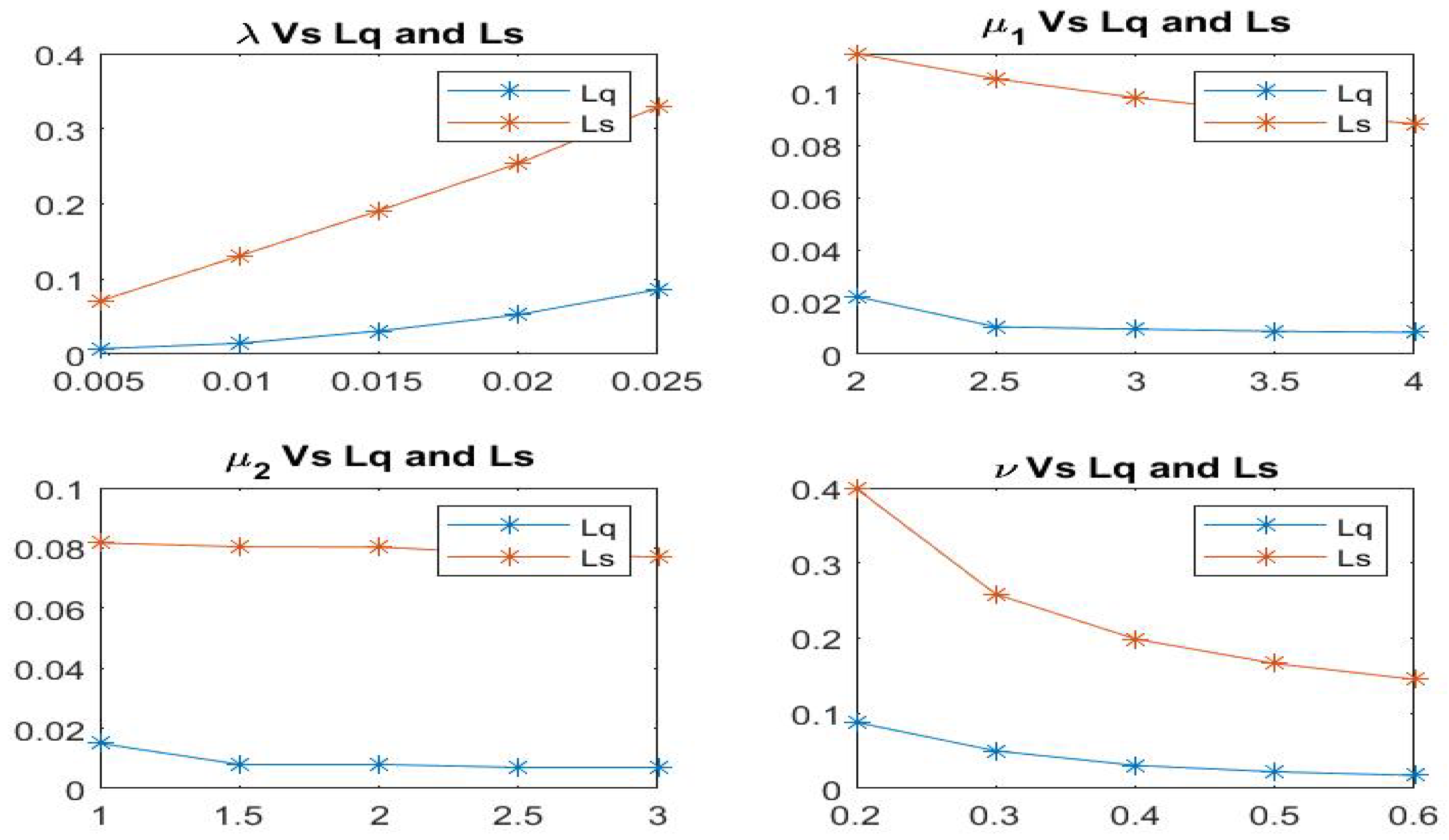
Table 5 clearly shows that, as the arrival rate λ increases, so do L s and L q , whereas, as the service rates μ 1 and μ 2 and feedback rates ν increase, L s and L q diminish.
Figure 2 reveals that, if the arrival rate rises, the average no. of customers throughout the system and queue will elevate, and if the service and feedback rates rises, the average no. of customers in the system and queue will diminish.
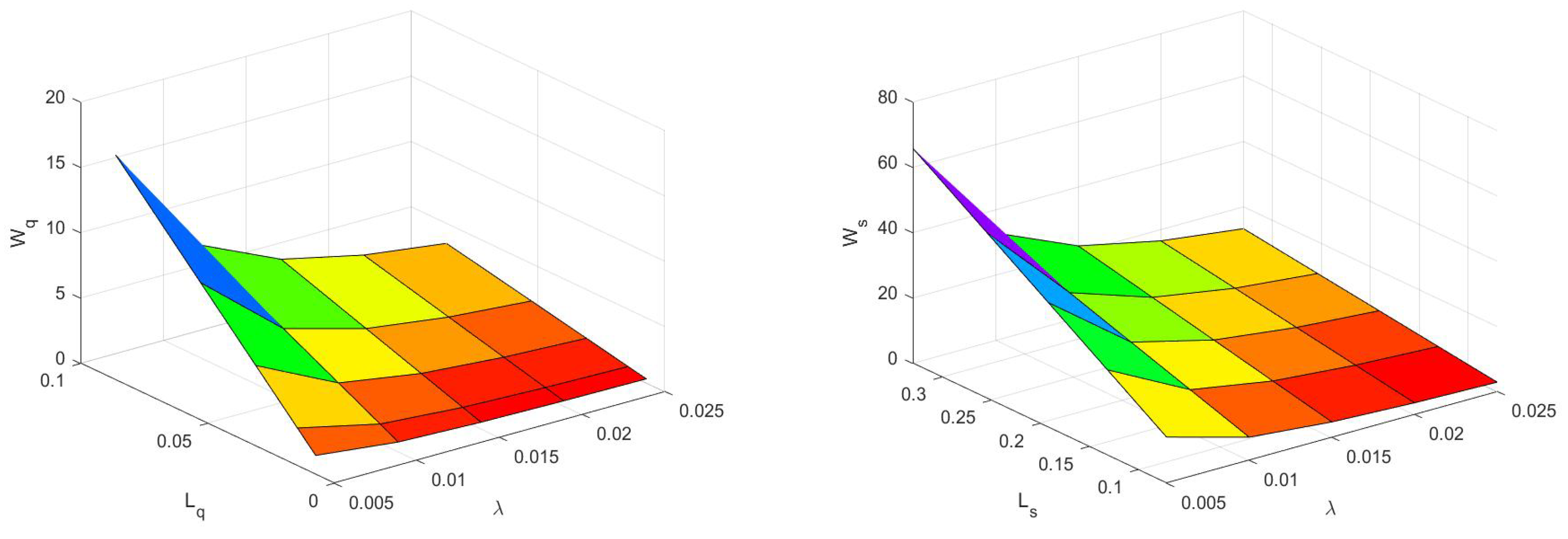
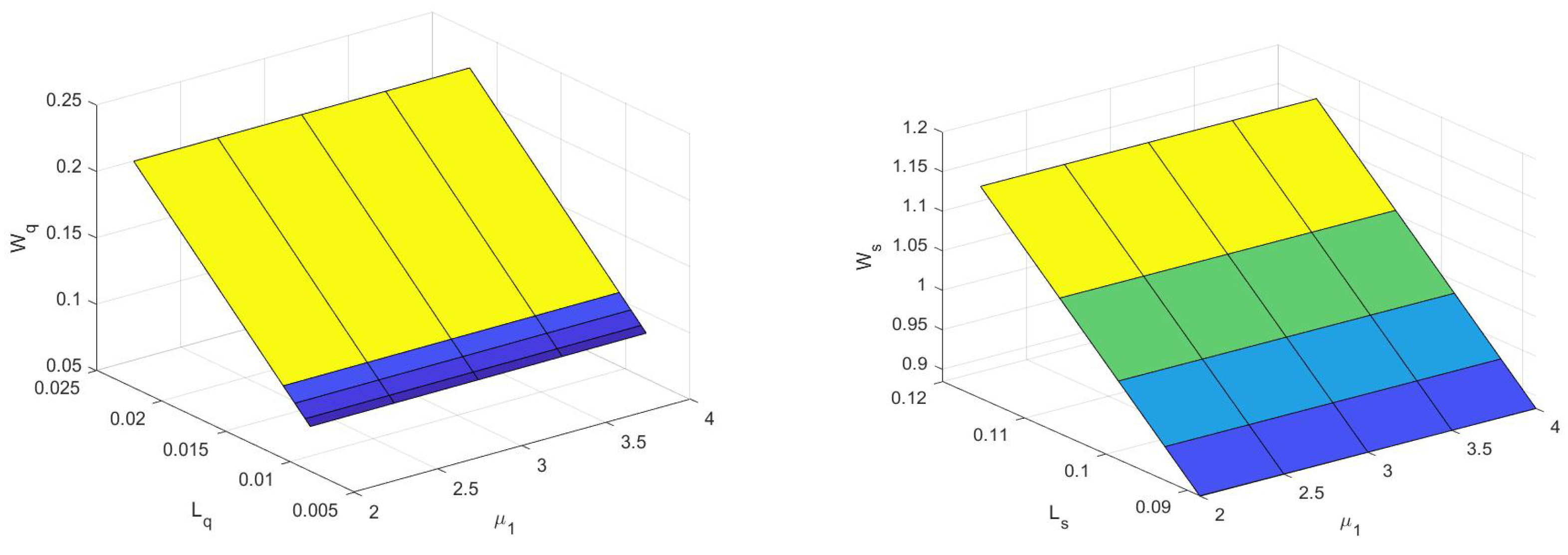
Figure 3, Figure 4, Figure 5 and Figure 6 display a three-dimensional graph of the system’s performance measures. Figure 3 reveals that, if the arrival rate rises, the average no. of customers throughout the system/queue and the average no. of customers waiting in the system/queue will elevate. Figure 4 and Figure 5 depict that, if server 1 and server 2’s service rate mounts, the average no. of customers throughout the system/queue and the average no. of customers waiting in the system/queue subside. Figure 6 reveals that, if the satisfied customers’ feedback rate is boosted, then the average no. of customers throughout the system/queue and the average no. of customers waiting in the system/queue will decline.

7. Conclusions

This paper investigated a two-server heterogeneous Markovian queueing system with an intermittently obtainable server and feedback under a hybrid vacation schedule. We extended the hybrid vacation idea of the model [32] with two servers under different service rates where one server is always available, and the other is only available on occasion. The matrix geometric approach was employed to derive the stationary condition and various performance measurements. The probability of the number of customers in the system and queue was also derived. In addition, the impact of system parameters was evaluated using numerical data. Furthermore, the conclusions gathered from numerical examples are valuable for developing results in a variety of authentic situations. The model under consideration is a generalized version of several emerging queueing models and is more realistic for queueing systems with human employees with various transmission rates. The proposed model can be enhanced in the future by incorporating additional features, such as the Markovian arrival process (MAP), phase-type arrival, multiple service and multi-stage services, optimal N-policy, and so on.

Author Contributions

Conceptualization and methodology, D.K. and I.K.; software, D.K.; validation, I.K.; formal analysis, I.K.; writing—original draft preparation, D.K.; writing—review and editing, I.K.; visualization, I.K.; supervision, I.K. All authors have read and agreed to the published version of the manuscript.

Funding

This research received no external funding.

Institutional Review Board Statement

Not applicable.

Informed Consent Statement

Not applicable.

Data Availability Statement

Not applicable.

Acknowledgments

The authors would like to thank Vellore Institute of Technology (VIT), for financial support.

Conflicts of Interest

The authors declare no conflict of interest.

Nomenclature

λ Arrival rate
μ 1 Server 1 service rate
μ 2 Server 2 service rate
μ v Lower service rate
θ v Mean of complete vacation duration
ξ The retrieval capacity rate
ζ 0 Probability of server 2 entering the working period from the complete vacation state
ν ¯ Feedback probability for an unsatisfied customer
ν Feedback probability for a satisfied customer
γ Breakdown rate
σ Repair rate
ϑ ( t ) Two-state Markov process at time t
N ( t ) No. of customers in the system at time t
S ( t ) Server 2 status at time t
HInfinitesimal generator matrix
A 00 , B 00 ,
C 00 , D 00 ,
D 11 , D 22 Sub-matrices of H
GSteady-state probability vector
RRate matrix
DLeast generator matrix
eColumn vector of 1s

References

  1. Morse, P.M. Queues, Inventories and Maintenance: The Analysis of Operational Systems with Variable Demand and Supply; Courier Corporation: Sydney, Australia, 2004. [Google Scholar]
  2. Singh, V.P. Two-server Markovian queues with balking: Heterogeneous vs. homogeneous servers. Oper. Res. 1970, 18, 145–159. [Google Scholar] [CrossRef]
  3. Krishnamoorthy, A.; Sreenivasan, C. An M/M/2 queueing system with heterogeneous servers including one with working vacation. Int. J. Stoch. Anal. 2012, 2012, 145867. [Google Scholar] [CrossRef] [Green Version]
  4. Indra; Rajan, V. Queuing analysis of markovian queue having two heterogeneous servers with catastrophes using matrix geometric technique. Int. J. Syst. Sci. 2017, 12, 205–212. [Google Scholar]
  5. Leemans, H. Waiting time distribution in a two-class two-server heterogeneous priority queue. Perform. Eval. 2001, 43, 133–150. [Google Scholar] [CrossRef]
  6. Mohammadi, A.; Salehi Rad, M.R. An M/G/1 queueing model with k sequential heterogeneous service steps and vacations in the transient state. Qual. Technol. Quant. Manag. 2022, 19, 633–647. [Google Scholar] [CrossRef]
  7. Seenivasan, M.; Indumathi, M. Performance Analysis of Two Heterogeneous Server Queuing Model with Intermittently Obtainable Server Using Matrix Geometric Method. J. Phys. Conf. Ser. 2021, 1724, 012001. [Google Scholar] [CrossRef]
  8. Agarwal, N.N. Some Problems in the Theory of Reliability and Queues. Ph.D.Thesis, Kurukshetra University, Kurukshetra, India, 1965. [Google Scholar]
  9. Sharda. A queuing problem with intermittently available server and arrivals and departures in batches of variable size. ZAMM 1968, 48, 471–476. [Google Scholar] [CrossRef]
  10. Seenivasan, M.; Senthilkumar, R.; Subasri, K.S. M/M/2 heterogeneous queueing system having unreliable server with catastrophes and restoration. Mater. Today Proc. 2022, 51, 2332–2338. [Google Scholar] [CrossRef]
  11. Levy, Y.; Yechiali, U. Utilization of idle time in an M/G/1 queueing system. Manag. Sci. 1975, 22, 202–211. [Google Scholar]
  12. Doshi, T. Queueing systems with vacations—A survey. Queueing Syst. 1986, 1, 29–66. [Google Scholar] [CrossRef]
  13. Takagi, H. Queueing analysis: A Foundation of Performance Evaluation; Vacation Priority Systems 1; North-Holland: Amsterdam, The Netherlands, 1991. [Google Scholar]
  14. Servi, L.D.; Finn, S.G. M/M/1 queues with working vacations (M/M/1/WV). Perform. Eval. 2002, 50, 41–52. [Google Scholar] [CrossRef]
  15. Tian, N.; Zhao, X.; Wang, K. The M/M/1 queue with single working vacation. Int. J. Inf. Manag. 2008, 19, 621–634. [Google Scholar]
  16. Ke, J.C.; Wu, C.H.; Zhang, Z.G. Recent developments in vacation queueing models: A short survey. Int. J. Oper. Res. 2010, 7, 3–8. [Google Scholar]
  17. Bouchentouf, A.A.; Boualem, M.; Yahiaoui, L.; Ahmad, H. A multi-station unreliable machine model with working vacation policy and customers’ impatience. Qual. Technol. Quant. Manag. 2022, 19, 766–796. [Google Scholar] [CrossRef]
  18. GnanaSekar, M.M.N.; Kandaiyan, I. Analysis of an M/G/1 Retrial Queue with Delayed Repair and Feedback under Working Vacation policy with Impatient Customers. Symmetry 2022, 14, 2024. [Google Scholar] [CrossRef]
  19. Zhang, Z.J.; Xu, X.L. Analysis for the M/M/1 queue with multiple working vacations and N-policy. Int. J. Inf. Manag. 2008, 19, 495–506. [Google Scholar]
  20. Mytalas, G.C.; Zazanis, M.A. Performance analysis for Bernoulli feedback queues subject to disasters: A system with batch Poisson arrivals under a multiple vacation policy. Qual. Technol. Quant. Manag. 2022, 1–34. [Google Scholar] [CrossRef]
  21. Neuts, M.F. Matrix-Geometric Solutions in Stochastic Models; JHU: Baltimore, MD, USA, 1981. [Google Scholar]
  22. Xu, X.; Zhang, Z.; Tian, N. The M/M/1 queue with single working vacation and set-up times. Int. J. Oper. Res. 2009, 6, 420–434. [Google Scholar]
  23. Vijayashree, K.V.; Ambika, K. An M/M/1 queue subject to differentiated vacation with partial interruption and customer impatience. Qual. Technol. Quant. Manag. 2021, 18, 657–682. [Google Scholar]
  24. Shekhar, C.; Varshney, S.; Kumar, A. Matrix-geometric solution of multi-server queueing systems with Bernoulli scheduled modified vacation and retention of reneged customers: A meta-heuristic approach. Qual. Technol. Quant. Manag. 2021, 18, 39–66. [Google Scholar] [CrossRef]
  25. Aniyeri, R.; Nadar, C.R. A multiphase queuing system with assorted servers by using matrix geometric method. Int. J. Appl. Eng. 2017, 12, 12052–12059. [Google Scholar]
  26. Federgrune, A.; Green, L. Queueing system with service interruptions. Oper. Res. 1986, 34, 752–768. [Google Scholar] [CrossRef]
  27. Jain, M.; Jain, A. Working vacations queueing model with multiple types of server breakdowns. Appl. Math. Model. 2010, 34, 1–13. [Google Scholar] [CrossRef]
  28. Kalyanaraman, R.; Seenivasan, M. Multi-server retrial queuing system with unreliable server. Int. J. Comput. Cogn. 2010, 7, 113–120. [Google Scholar]
  29. Renisagaya Raj, M.; Chandrasekar, B. Matrix-Geometric Method for Queueing Model with Subject to Breakdown and N-Policy Vacations. Int. J. Math. Aeterna 2015, 5, 917–926. [Google Scholar]
  30. Subramanian, A.M.G.; Ayyappan, G.; Sekar, G. M/M/1 Retrial queueing System with Pre-emptive priority service. Int. J. Comput. Appl. 2010, 4, 2379–2389. [Google Scholar]
  31. Sharma, S.K.; Kumar, R. A single-server Markovian feedback queuing system with discouraged arrivals and retention of reneged customers. Am. J. Oper. Res. 2013, 4, 35–39. [Google Scholar]
  32. Anshul, K.; Jain, M. Cost Optimization of an Unreliable server queue with two stage service process under hybrid vacation policy. Math. Comput. Simul. 2022, 204, 259–281. [Google Scholar]
  33. Latouche, G.; Ramaswami, V. Introduction to matrix analytic methods in stochastic modeling. SIAM J. Comp. 1999. [Google Scholar] [CrossRef]
  34. Seenivasan, M.; Manikandan, H.; Subasri, K.S. Analysis of Heterogeneous Queueing Model with Unreliable Server and Working Vacation. Adv. Electr. Comput. 2022, 881, 331–345. [Google Scholar]
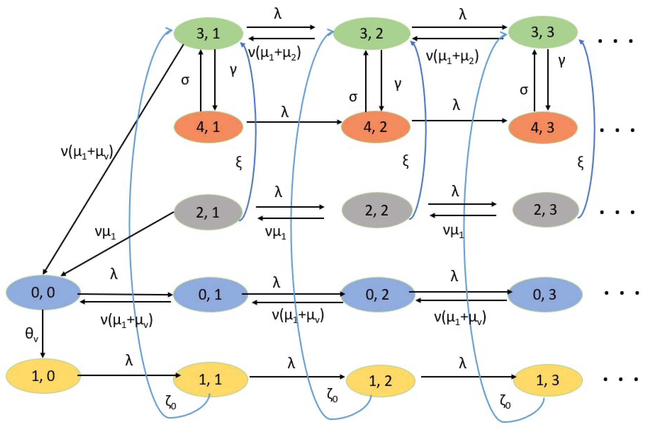
Figure 1. Transition diagram of the model.
Symmetry 15 01304 g001
Figure 2. Length of the system and queue size vs. parameters λ , μ 1 , μ 2 , ν .
Symmetry 15 01304 g002
Figure 3. Arrival rate λ vs. L q , W q , and arrival rate λ vs. L s , W s .
Symmetry 15 01304 g003
Figure 4. Service rate μ 1 vs. L q and W q , and service rate μ 1 vs. L s and W s .
Symmetry 15 01304 g004
Figure 5. Service rate μ 2 vs. L q and W q , and service rate μ 2 vs. L s and W s .
Symmetry 15 01304 g005
Figure 6. L q and W q vs. feedback rate ν , and L s and W s vs. feedback rate ν .
Symmetry 15 01304 g006
Table 1. Probability vector for λ .
λ 0.050.10.150.20.25
G 0 0.93300.88330.83960.79820.7566
G 1 0.06290.10310.13370.15840.1789
G 2 0.00390.01210.02250.03430.0477
G 3 0.00000.00120.00360.00720.0125
G 4 0.00000.00000.00040.00130.0034
G 5 0.00000.00000.00000.00000.0008
Total0.99980.99970.99980.99940.9999
Table 2. Probability vector for μ 1 .
μ 1 22.533.54
G 0 0.89590.90460.91100.91590.9198
G 1 0.09270.08540.07990.07570.0722
G 2 0.01010.00890.00820.00760.0072
G 3 0.00080.00080.00070.00060.0006
G 4 0.00000.00000.00000.00000.0000
Total0.99950.99970.99980.99980.9998
Table 3. Probability vector for μ 2 .
μ 2 11.522.53
G 0 0.92570.92690.92700.93890.9298
G 1 0.06700.06590.06580.06410.0634
G 2 0.00660.00650.00650.00620.0062
G 3 0.00050.00050.00050.00050.0004
G 4 0.00000.00000.00000.00000.0000
Total0.99980.99980.99980.99970.9998
Table 4. Probability vector for ν .
ν 0.20.30.40.50.6
G 0 0.70800.79080.83140.85570.8718
G 1 0.21120.16810.14170.12430.1121
G 2 0.05900.03330.02270.01730.0141
G 3 0.01600.00640.00340.00230.0015
G 4 0.00420.00100.00040.00010.0015
G 5 0.00100.00010.00000.00000.0001
Total0.99940.99970.99960.99970.9996
Table 5. Effect of λ , μ 1 , μ 2 , and ν on performance measures.
λ P S I d P S 2 W v P S 2 C v P S 2 I o P S 2 W k P S 2 B d E N 1 E N 2 E N 3 E N 4 E N 5 L s E N q 1 E N q 2 E N q 3 E N q 4 E N q 5 L q
0.050.93300.32420.65130.00000.01950.00480.01200.03230.00000.02110.00530.07070.00040.00140.00000.00160.00390.0073
0.10.88330.48340.47780.00000.03120.00730.03700.04760.00000.03730.00900.13090.00250.00420.00000.00610.00170.0145
0.150.83960.58180.36810.00000.04070.00920.06950.05490.00000.05410.01260.19110.00720.00690.00000.01340.00340.0309
0.20.79820.65200.28710.00000.04990.01040.10830.0570.00000.07310.01540.25380.01520.00920.00000.02320.00500.0526
0.250.75660.70890.21790.00000.06140.01170.1540.05430.00000.10150.01960.32940.02740.01070.00000.04010.00790.0861
μ 1 P S I d P S 2 W v P S 2 C v P S 2 I o P S 2 W k P S 2 B d E N 1 E N 2 E N 3 E N 4 E N 5 L s E N q 1 E N q 2 E N q 3 E N q 4 E N q 5 L q
20.89590.48370.48370.00000.02600.00610.02910.04810.00000.03070.00740.11530.00150.00420.00000.00470.01170.0221
2.50.90460.48450.48740.00000.02250.00530.0240.04860.00000.02660.00640.10560.0010.00430.00000.00410.00110.0105
30.91100.48580.48950.00000.01980.00470.02060.04880.00000.02330.00570.09840.00080.00430.00000.00350.0010.0096
3.50.91590.48720.49070.00000.01770.00420.0180.04890.00000.02070.00510.09270.00060.00430.00000.0030.00090.0088
40.91980.48880.49110.00000.01610.00380.01600.04890.00000.01890.00460.08840.00050.00430.00000.00280.00080.0084
μ 2 P S I d P S 2 W v P S 2 C v P S 2 I o P S 2 W k P S 2 B d E N 1 E N 2 E N 3 E N 4 E N 5 L s E N q 1 E N q 2 E N q 3 E N q 4 E N q 5 L q
10.92570.49270.49030.00000.01370.00310.01310.04880.00000.01620.00360.08170.00030.00430.00000.00250.00760.0147
1.50.92690.49550.48860.00000.01280.00290.01310.04870.00000.01520.00340.08040.00030.00430.00000.00240.00050.0075
20.9270.47470.50970.00000.01260.00280.01150.05060.00000.01500.00320.08030.00030.00440.00000.00240.00040.0075
2.50.92890.50170.48410.00000.01140.00250.01330.04810.00000.01370.00290.07800.00030.00420.00000.00230.00040.0072
30.92980.50540.48120.00000.01080.00240.01340.04790.00000.01290.00280.07700.00030.00420.00000.00210.00040.0070
ν P S I d P S 2 W v P S 2 C v P S 2 I o P S 2 W k P S 2 B d E N 1 E N 2 E N 3 E N 4 E N 5 L s E N q 1 E N q 2 E N q 3 E N q 4 E N q 5 L q
0.20.7080.48370.37970.00000.11140.02460.16030.03810.00000.16480.03580.39900.02250.00090.00000.05340.01120.0880
0.30.79080.48250.42750.00000.07290.01680.09630.04260.00000.09700.02250.25840.01590.00380.00000.02410.00570.0495
0.40.83140.48210.45040.00000.05430.01280.06870.04490.00000.06860.01670.19890.00850.00400.00000.01430.00390.0307
0.50.85570.48230.46360.00000.04350.01030.05320.04620.00000.05370.01310.16620.00510.00410.00000.01020.00280.0222
0.60.87180.48280.47200.00000.03630.00850.04370.04690.00000.04410.01050.14520.00350.00410.00000.00780.00200.0174
Disclaimer/Publisher’s Note: The statements, opinions and data contained in all publications are solely those of the individual author(s) and contributor(s) and not of MDPI and/or the editor(s). MDPI and/or the editor(s) disclaim responsibility for any injury to people or property resulting from any ideas, methods, instructions or products referred to in the content.