Temporal Network Link Prediction Based on the Optimized Exponential Smoothing Model and Node Interaction Entropy

Abstract

Link prediction accuracy in temporal networks is easily affected by the time granularity of network snapshots. This is due to the insufficient information conveyed by snapshots and the lack of temporal continuity between snapshots. We propose a temporal network link prediction method based on the optimized exponential smoothing model and node interaction entropy (OESMNIE). This method utilizes fine-grained interaction information between nodes within snapshot periods and incorporates the information entropy theory to improve the construction of node similarity in the gravity model as well as the prediction process of node similarity. Experiment results on several real-world datasets demonstrate the superiority and reliability of this proposed method in adapting to link prediction requirements over other methods across different time granularities of snapshots, which is essential for studying the evolution of temporal networks.

1. Introduction

The complex network model is an abstract approach to analyzing real-world interactions between objects in the form of points and lines [1]. Any individual in nature can be connected with another in a specific relation. With different observation scales, the expression range of a complex network can be applied to different fields. Complex networks can express any chemical structure [2] or microscopic biological structure [3] by taking molecules and cells as individuals. By shrinking the scale to neurons, the complex network can also express the structure of the human brain [4]. By abstracting the sensors used in autonomous driving as nodes, the complex network can be represented as a road topology within a specific area [5]. Thus, a series of complex network techniques can be further used to analyze the target system features, such as node importance evaluation [6], fractal research of complex networks [7], and community detection [8]. As one of the most representative problems in complex networks, link prediction aims to estimate the unknown or missing links possibility between nodes by using the current node connection information of the target network.

Link prediction can more accurately represent interaction principle and help people to efficiently understand evolutionary trends and mechanisms of the target network [9]. Additionally, link prediction results have many applications in current society. Link prediction matching between user demand and hotel conditions can improve hotel revenue [10]. The link prediction in wireless sensor networks (WSNs) can improve the information transmission efficiency while maintaining relatively low re-transmission rates for energy-saving purposes [11]. The link prediction analysis in the disease–gene interaction network can help the pharmaceutical industry develop targeted drugs [12].

The processing objects of link prediction have been diversified, including static networks, dynamic networks, temporal networks, heterogeneous networks, heterogeneous temporal networks, and hypergraphs. There are five primary methods for temporal network link prediction: matrix factorization, probability, spectral clustering, machine learning, and time series [13]. In matrix factorization, most methods are based on nonnegative matrix factorization (NMF). Sheng et al. [14] propose a temporal link prediction method based on NMF. This method considers three aspects: the global structure of nodes, the local information of nodes, and the attributes of nodes. By leveraging multiple sources of information, this method predicts the probability of link occurrence. In probability, the uncertainty and variability of links among nodes are typically quantified using the maximum likelihood approaches or probability distributions. Based on the concept of Markov chains, the extended temporal exponential random graph model (etERGM) [15] can predict the future attributes and connections of nodes based on historical data. In spectral clustering, Fang et al. proposed a time regression model for temporal link prediction. The idea is to integrate the spectral graph theory and low-rank approximation into a time series model, allowing the model to capture more graph information and improve the accuracy of temporal link prediction. In machine learning, network representation learning (NRL) utilizes various graph embedding algorithms to represent all properties of temporal network in a low-dimensional vector space. This approach effectively eliminates the challenges associated with extracting features of snapshots. By leveraging these low-dimension feature vectors, temporal link prediction can be performed well. Zhou et al. [16] proposed a NRL method called DynamicTriad, which simulates the occurrence of triadic closure processes among nodes. This enables the model to capture temporal features and obtain vector representation for each node across different periods. In time series-based temporal link prediction, researchers have proposed various methods to enhance the accuracy of temporal link prediction by obtaining the local similarity of nodes in different ways. Huang et al. [17] used specific time granularity to treat temporal network data sets into snapshots. They proposed an improved gravity model with second-order neighbors, denoted by gravity (GR), to compute the score matrix in each static network snapshot. All score matrices will be combined with a time attenuation factor to accumulate the next period connection probability. Yang et al. [18] proposed a temporal network link prediction method, tensor-based node similarity (TBNS). The TBNS treats the collection of snapshots with time dimension as a three-dimensional tensor and employs the exponential smoothing model to compress a three-dimensional tensor into a two-dimensional node similarity matrix, which serves as the link prediction scores for the next period. This approach addresses the problem that snapshots cannot capture node connectivity strength due to the large time granularity sizes. However, capturing any microscopic connections in this approach will likely to lead to many sparse matrices, which wastes storage space. Güneş et al. [19] first calculated the nodes similarity indexes in different periods by common neighbors, preferential attachment, Adamic–Adar, and the Jaccard indicator. Then, they used the autoregressive integrated moving average (ARIMA) to predict the similarity between nodes for the future.

All of the above time series-based temporal link predictions [17,18,19] follow the framework processing rules shown in Figure 1. First, the temporal network represents different snapshots at different periods. Second, the network snapshot in each layer can construct nodes’ similarity matrix in different ways. Finally, various numerical prediction models are used to predict the snapshot similarity matrix at a future time. Therefore, constructing reasonable node similarity is crucial in improving the accuracy of time series-based network temporal link prediction methods.

Table 1. A brief summary of some existing link prediction method based on node similarity.

Indicator	Topology	Definition 1	Complexity 2
CN [20]	Local	$S_{xy}=\Gamma \left(x\right)\cap \Gamma \left(y\right)$	$O\left(n^2\right)$
Jaccard [21]	Local	$S_{xy}=\frac{\Gamma \left(x\right)\cap \Gamma \left(y\right)}{\Gamma \left(x\right)\cup \Gamma \left(y\right)}$	$O\left(n^2\right)$
HPI [22]	Local	$S_{xy}=\frac{\left|\Gamma \left(x\right)\cap \Gamma \left(y\right)\right|}{\min \left(k_x,k_y\right)}$	$O\left(n^2\right)$
HPD [23]	Local	$S_{xy}=\frac{\left|\Gamma \left(x\right)\cap \Gamma \left(y\right)\right|}{\max \left(k_x,k_y\right)}$	$O\left(n^2\right)$
AA [24]	Local	$S_{xy}={{\displaystyle \sum }}_{Z\in \Gamma \left(x\right)\cap \Gamma \left(y\right)}\frac{1}{\log \left(k_Z\right)}$	$O\left(2n^2\right)$
RA [25]	Local	$S_{xy}={{\displaystyle \sum }}_{Z\in \Gamma \left(x\right)\cap \Gamma \left(y\right)}\frac{1}{k_Z}$	$O\left(2n^2\right)$
PA [26]	Local	$S_{xy}=k_x{k}_y$	$O\left(2n\right)$
GR [17]	Local	$S_{xy}={{\displaystyle \sum }}_{Z\in \Gamma \left(x\right)\cap \Gamma \left(y\right)}\frac{G_{i,Z}·G_{Z,j}}{{\delta }^2}$	$O\left(n^2\right)$
LP [27]	Semi-Local	$S=A^2+\alpha ·A^3$	$O\left(n^3\right)$
LRW [28]	Semi-Local	$S_{xy}\left(t\right)=q_x·{\pi }_{xy}\left(t\right)+q_y·{\pi }_{yx}\left(t\right)$	$O\left(n{k}^t\right)$
RWR [28]	Semi-Local	$S_{xy}\left(t\right)=q_{xy}+q_{yx}$	$O\left(n^3\right)$
Cos+ [29]	Global	$S_{xy}=\frac{l_{xy}^{+}}{\sqrt{l_{xx}^{+}·l_{yy}^{+}}}$	$O\left(n^3\right)$
ACT [30]	Global	$S_{xy}=\frac{1}{l_{xx}^{+}+l_{yy}^{+}-2l_{xy}^{+}}$	$O\left(n^3\right)$

Note: ¹ $\Gamma \left(x\right)$ and $\Gamma \left(y\right)$ represent the neighbors of node $x$ and node $y$; $k_x$ and $k_y$ are the degree of node $x$ and node $y$; $A$ is the adjacency matrix of the network; $S$ is a matrix composed of elements representing the similarity between nodes in the network; $l_{xy}^{+}$ denotes the element in the row $x$ and column $y$ of pseudo-inverse matrix $L^{+}$; $\alpha$ denotes a decay factor, which allows controlling the contribution of third-order neighbors to the similarity of nodes; ${\pi }_{xy}\left(t\right)$ denote the random walk probability from node $x$ and node $y$ at time $t$; $G_{i,Z}$ is the gravitational force between node $x$ and node $y$; ² $n$ denotes the number of nodes in the network; $k$ is the average degree of nodes; and $t$ is the step of random walk steps.

briefly highlights some existing node similarity-based link prediction methods.

However, the link prediction idea of using the network snapshots as a time series prediction needs to be improved. The network snapshot is an adjacency matrix format. Multiple joins within a time granularity $L$ will be recorded in a binary form. In temporal networks, the interaction information is represented using the triplet format $\left(i,j,t\right)$. The time granularity $L$ will divide time stamps $t$ into $n$ slices of snapshots. Each network snapshot contains interaction events within the corresponding period. In the temporal prediction process, there may be misjudgments in the reference scores of the similarity matrix among nodes within each snapshot. For example, during the snapshot period, some nodes may have lower interaction strength, and as a result, their similarity may not provide more weight for the time series forecasting model. A large time granularity $L$ can provide more edge information for snapshots, but it can also destroy the accuracy of reference scores for similarity among nodes during the prediction process. The time series-based temporal link prediction method [17,18,19] mentioned above enhances the expressive capacity of network snapshots and improves the computational speed of the algorithm by considering the local information of node. Regardless, large time granularity may not guarantee the algorithm’s accuracy [31]. To address the above problems, we propose a temporal network link prediction method based on optimized exponential smoothing model and node interaction entropy (OESMNIE). The OESMNIE method considers the fine-grained interaction information among nodes within a snapshot and the impact of interaction intensity on node similarity in the time series prediction process. The OEMNIE method leverages the characteristics of wide-ranging and low-frequency node interactions within a snapshot, combined with information entropy, to further differentiate the popularity of nodes within the snapshot structure, thereby enhancing the accuracy of constructing node similarity based on the gravity model. Furthermore, the OESMNIE method normalizes the sum of interaction entropy for each node within the snapshot and incorporates the smoothing coefficient from the exponential smoothing model. This allows the prediction of node similarity to dynamically weight according to the overall trend of network interactions, and the three-dimensional snapshot similarity tensor is eventually compressed into a two-dimensional node similarity matrix (i.e., future link prediction scores). This provides a new idea for modeling time series-based temporal link prediction.

The major contributions are summarized as follows:

• We record the fine-grained interaction information among nodes within the snapshot period and incorporate the concept of information entropy and weak ties to construct the node interaction entropy. This value differentiates the popularity of nodes within the snapshot structure from a more nuanced perspective.
• We combine node interaction entropy and eigenvector centrality to construct an enhanced node similarity that considers the network structure’s distance between nodes, weak ties characteristics, and centrality.
• We normalized the sum of node interaction entropy, and the normalized result will reflect the ratio of the current snapshot’s weak ties during the entire period. With the higher ratio, the node similarity matrices can provide more weights for time series prediction. We combine the smoothing coefficient and the ratio into the exponential smoothing model. This improves the shortcoming of the single reference score of the prediction process.

The remaining content of this paper is divided into several parts. In Section 2, we will highlight the related works, introduce the concepts of temporal networks, network snapshots, and multi-layer network model, as well as explain weak ties theory, gravity model, information entropy, eigenvector centrality of nodes, temporal network link prediction method, and the role of exponential smoothing model in link prediction. Section 3 will provide a more detailed description of the OESMNIE method proposed in this paper. Section 4 will include specific comparative experimental analysis and discussion. Finally, Section 5 will conclude this paper.

2. Related Works

2.1. Temporal Network

The interactions between nodes in the temporal network are continuously changing. We make a simplifying assumption: the increase and decrease in nodes is not yet considered for the analyzed network. Therefore, temporal network is generally defined as $G=\left(V,E_t\right)$, where $V$ is the node set $\left\{v_1,v_2,v_3,\dots ,v_n\right\}$ in the temporal network. $E$ represents the connection of the temporal network edges over the whole period. $E_t$ contains all nodes’ interaction information in the recorded period, and $E_t$ can be represented as set of triples with time stamp, $E_t=\left\{\left(v_1,v_2,t_0\right),\dots ,\left(v_i,v_j,t_n\right)\right\}$, where $t_n$ indicates that there is a connection between two nodes at the $n$ instant.

2.2. Construction of Network Snapshots and Multi-Layer Network Model

In order to make a link prediction model based on time series to analyze the transformed temporal network, time granularity with an appropriate span $L$ is generally adopted to record and divide the entire period of the temporal network. $L$ can sequentially divide interaction information by hours, minutes, seconds, days, months, or years. Consequently, the adjacency matrix $A_n$ represents the record of whether there is any interaction between nodes within time granularity $L$. Network snapshots $A_n$ at different time will contain different edges subsets $E_n^{\prime }$, and $E_n^{\prime }$ can be expressed by $E_n^{\prime }=\left\{\left(v_i,v_j,t_{nL}\right),\dots ,\left(v_i,v_j,t_{\left(n+1\right)L}\right)\right\}$. The temporal network snapshot is constructed as in Equation (1).

$$A_n\left(i,j\right)=\left\{\begin{array}{c}1 if E_n^{\prime }\left(i,j,t\right)\in E\left[\left(n\right)L,\left(n+1\right)L\right]\\ 0 if E_n^{\prime }\left(i,j,t\right)\notin E\left[\left(n\right)L,\left(n+1\right)L\right]\end{array}\right.$$

(1)

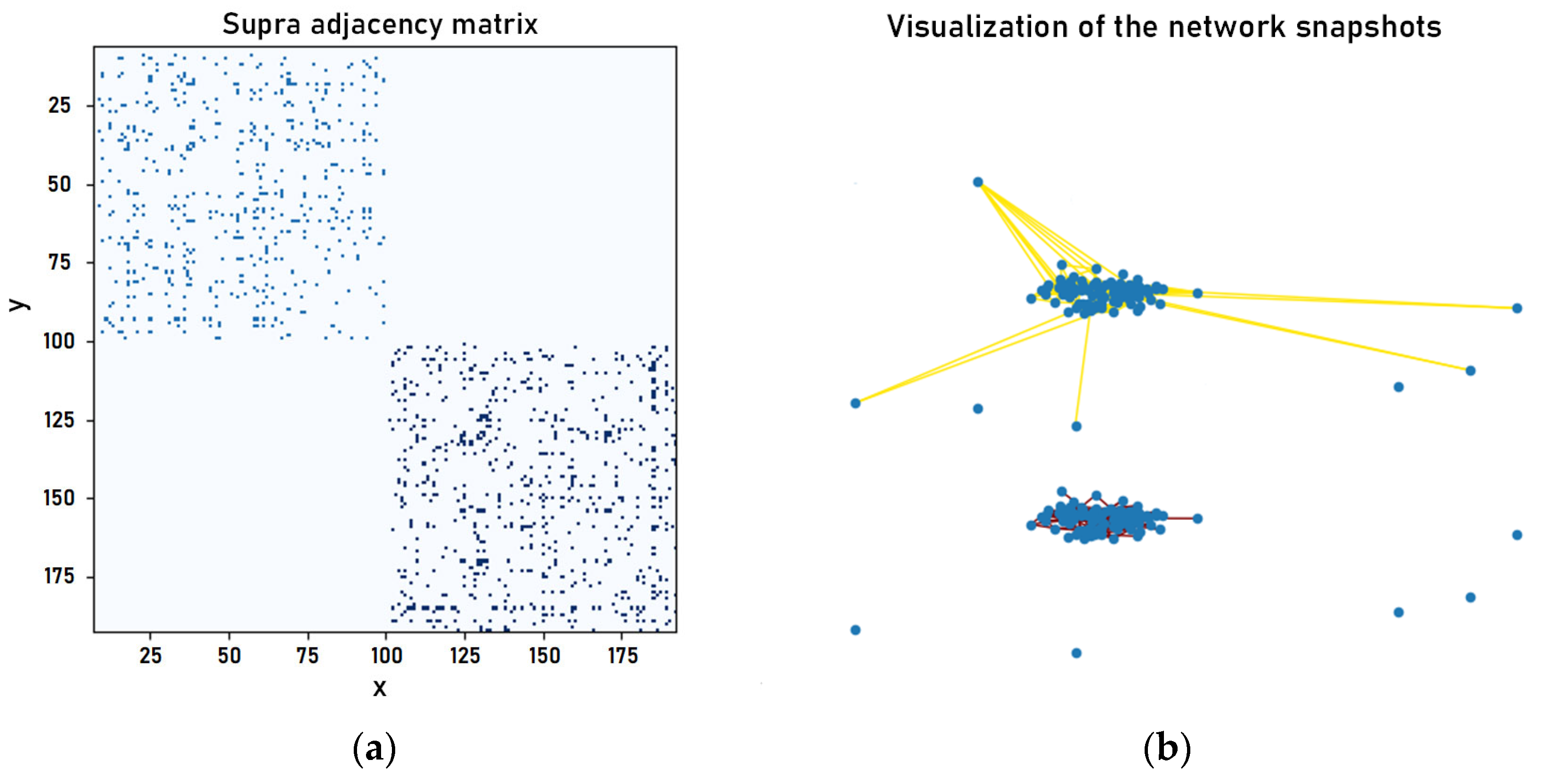
where, $E_n^{\prime }\left(i,j,t\right)\in E\left[\left(n\right)L,\left(n+1\right)L\right]$ represents that node $i$ and node $j$ are connected in $\left[\left(n\right)L,\left(n+1\right)L\right]$ period. We can obtain a symmetric adjacency matrix containing the connection information for a period. The multi-layer network model is constructed from multiple network snapshots taken at different periods, forming a tensor with a temporal dimension. The multi-layer network model is also widely used for representing heterogeneous networks. The specific format can be shown in Figure 2 using the supra-adjacency matrix (SAM) model proposed by Taylor [32]. The SAM model can arrange the adjacency matrices (network snapshots) of different periods in chronological order along the diagonal. We have removed the interlayer relationship matrix from the SAM model, using it solely as a visualization tool for network snapshots.

By partitioning the temporal network using network snapshots, we can analyze the evolution process of the temporal network.

2.3. Weak Ties Theory

Weak ties theory [33,34] primarily focuses on the connection frequency characteristics of nodes and divides nodes’ interaction characteristics into strong and weak ties. Strong ties shows that nodes’ interactions are large, and the range is relatively stable. Weak ties shows that nodes’ interactions are less, but the range is relatively wider. The theory states that weak ties are easier to traverse different social groups than strong ties. In other words, nodes with weak ties can transfer information from one group to another, breaking down information silos. Additionally, these nodes are typically connected to multiple communities, and their actions and statements are more likely to influence others. Therefore, they have a more significant impact and information dissemination effect. Lü et al. [35] introduced a free parameter $\alpha$ to control the relatively contribution of weak ties in node similarity measure. The result shows that link prediction accuracy can be effectively improved by introducing weak ties.

2.4. The Gravity Model

Levy et al. [36] performed an analysis on four networks with the small-world property. They confirmed that there is a dependency between the connection probability and distance. Moreover, all the four networks show the same empirical law: the probability of connection between nodes in social networks is inversely proportional to the square of the distance, which is similar to the dependence of Newton’s law of universal gravity on distance. Wahid-Ul-Ashraf et al. [37] used network science’s measurement method to obtain the shortest path, inverse Katz score between nodes, and different node centrality measures, which are introduced into Newton’s law of universal gravity as distance and quality. They constructed new node similarity measures and proved the feasibility of physical models in link prediction. The gravity model is shown in Equation (2).

$$Score\left(v_i,v_j\right)\propto \frac{F\left(v_i\right)·F\left(v_j\right)}{D{\left(v_i,v_j\right)}^2}$$

(2)

where, $F\left(v_i\right)$ can be different kinds of indicator used to evaluate node influence, including but not limited to degree centrality (DC), closeness centrality (CC), betweenness centrality (BC), eigenvector centrality (EC), and others. $D\left(v_i,v_j\right)$ is distance between node $v_i$ and node $v_j$.

2.5. Information Entropy

Information entropy is a vital concept in information theory used to measure the uncertainty or information content of a random variable. Therefore, when we use information entropy to measure a system, we focus on statistically analyzing all the states that occur in the system and converting the occurrence frequencies of events into probabilities. A high information entropy of a system indicates a more variety of event states occurring, and that the probabilities of different events are relatively dispersed. Conversely, a low information entropy of a system implies a more limited range of event states occurring, and that certain events have higher probabilities of occurrence. The information entropy method can be used to quantify the link prediction problems based on a probability description. There are several entropy weight methods that have been proposed for link prediction research, such as the node similarity index of path entropy [38], structural entropy model [39], link prediction method based on relative entropy [40], and maximum entropy model [41]. The calculation process of information entropy is expressed as Equation (3).

$$H\left(X\right)=-{\displaystyle \sum }_{i}P\left(x_i\right)\log \left(P\left(x_i\right)\right)$$

(3)

where, $X$ the entire target system, which includes all the events covered within the system, denoted as $X=\left\{x_1,x_2,\dots ,x_n\right\}$. $P\left(x_i\right)$ is the probability of the occurrence of the event $x_i$.

2.6. The Eigenvector Centrality of Nodes

The eigenvector centrality was proposed by Bonacich [42]. According to the eigenvector centrality of node, the node’s eigenvector centrality depends on the number of the target node’s neighbor nodes and the centrality of neighbor nodes. The specific calculation process is shown in Equation (4).

$$EC\left(i\right)=D\left(i\right)=\frac{1}{c}{\displaystyle \sum }_j^{\tau \left(i\right)}A\left(i,j\right)\times D\left(j\right)$$

(4)

The node’s eigenvector centrality can be succinctly expressed as a one-dimensional vector of length $N$ (it is equal to the number of nodes in network), where each element represents the centrality score of a node. According to the calculation approach defined by Equation (4), the centrality of node $i$ is determined by the sum of centrality scores of its neighboring nodes. The final node centrality is obtained by iteratively computing this process until the eigenvector centrality converges. This process transfers and accumulates the centrality information of nodes within the network to reflect their importance and influence.

2.7. Temporal Network Link Prediction

With the diversification of modeling methods, link prediction can be divided into two categories: static network link prediction and dynamic network link prediction. Static network link prediction involves analyzing and supplementing unknown or missing edge information using the existing edge set $E$ in a given analysis network $G\left(V,E\right)$. On the other hand, dynamic network link prediction aims to predict the connection status at time $T+1$ based on the $E_n^{\prime }$ from $0$ to $T$. Therefore, historical edge information plays an essential role in predicting future connections.

2.8. The Exponential Smoothing Model in Link Prediction

The exponential smoothing model, derived from the moving average model, is a numerical prediction model. The temporal network link prediction method based on the exponential smoothing model takes each snapshot adjacency matrix as a dataset and introduces smoothing coefficient $\alpha$ to compress the whole temporal snapshot matrix, which is a three-dimensional tensor, into a two-dimensional matrix. The score of the last compressed matrix is used as the link prediction score for the next period. The specific exponential smoothing model applied to link prediction is given in Equation (5).

$$\begin{array}{c}{S}_1=A_0\hfill \\ S_{T+1}=\alpha A_T+\left(1-\alpha \right)S_T\hfill \\ Z_{T+1}=\begin{array}{c}\left[\begin{array}{ccc}\begin{array}{cc}{S}_{T+1}^{1,1}& S_{T+1}^{1,2}\\ S_{T+1}^{2,1}& S_{T+1}^{2,2}\end{array}& \dots & \begin{array}{c}{S}_{T+1}^{1,n}\\ S_{T+1}^{2,n}\end{array}\\ ⋮& \ddots & ⋮\\ \begin{array}{cc}{S}_{T+1}^{n,1}& S_{T+1}^{n,2}\end{array}& \dots & S_{T+1}^{n,n}\end{array}\right]·\left[\begin{array}{ccc}\begin{array}{cc}{S}_{T+1}^{1,1}& S_{T+1}^{1,2}\\ S_{T+1}^{2,1}& S_{T+1}^{2,2}\end{array}& \dots & \begin{array}{c}{S}_{T+1}^{1,n}\\ S_{T+1}^{2,n}\end{array}\\ ⋮& \ddots & ⋮\\ \begin{array}{cc}{S}_{T+1}^{n,1}& S_{T+1}^{n,2}\end{array}& \dots & S_{T+1}^{n,n}\end{array}\right]\end{array}\hfill \end{array}$$

(5)

where, $A_T$ is the network snapshot (adjacency matrix) at period $T$, $S_{T+1}$ is the node similarity matrix of the snapshot $A_{T+1}$, and the smoothing coefficient $\alpha$’s range is $\left[0,1\right]$. The model provides a reference score $\alpha$ for the snapshot in the recent period, and the remaining $\left(1-\alpha \right)$ scores will be the historical connection information reference scores. By compressing the historical connection information of each node, the observation angle starts from the current existing link. The current snapshot’s similarity matrix will be the given score $\alpha$, and the remaining scores $\left(1-\alpha \right)$ will gradually diminish the contribution of the historical connection information in the prediction. Finally, the connection probability matrix $Z_{T+1}$ at the last time $T+1$ will depend on the final compressed node similarity matrix.

3. Description of the OESMNIE Temporal Network Link Prediction Method

3.1. Establishment of the Node Interaction Entropy

Link prediction methods based on network snapshots typically focus on the topology structure within the snapshots, while overlooking the potential correlation between node influence intensity and their connection frequency [43]. From the above problem, it is feasible to consider fine-grained interaction information between nodes and utilize a gravity model to construct node similarity for link prediction under network snapshots. Therefore, we conduct a statistical analysis of the frequency and range of interactions between nodes in each snapshot period and analyze the role of weak ties in characterizing node influence. In our daily lives, nodes with weak ties are widespread, such as supermarket salespeople. Although we may not interact with them frequently, they can act as bridge nodes, connecting multiple communities with low interaction frequency but a broad interaction range (e.g., interacting with lawyers, workers, police officers, and other diverse groups). The message will spread across multiple communities if these nodes are involved in information dissemination or viral propagation.

Conversely, suppose the message is disseminated to nodes with high interaction frequency and a narrow interaction range (e.g., nodes with strong ties). In that case, these nodes are more inclined to transmit information within their community. Therefore, nodes with weak ties generally have greater influence. To measure weak ties of nodes, we naturally consider the application of information entropy to assess system uncertainty. The interaction range of a node determines the number of events occurring in the system observed from that node, while the ratio of interaction frequency to total interactions can be seen as the probability of each connected event occurrence. Therefore, while constructing network snapshots, we also constructed a symmetric snapshot interaction frequency matrix $C_n$ and combined it with the concept of information entropy to create the node interaction entropy for different periods. This allows us to analyze the influence of nodes within each period based on fine-grained interaction behaviors, which can be further utilized for link prediction. The snapshot interaction frequency matrix $C_n$ is calculated using Equation (6).

$$C_n\left(i,j\right)=\left\{\begin{array}{c}+1 if E_n^{\prime }\left(i,j,t\right)\in E\left[\left(n\right)L,\left(n+1\right)L\right]\\ +0 if E_n^{\prime }\left(i,j,t\right)\notin E\left[\left(n\right)L,\left(n+1\right)L\right]\end{array}\right.$$

(6)

Once the node interaction frequency matrix $C_n$ corresponding to each snapshot is obtained, we can probabilistically transform each node’s interaction events. The specific process is shown in Equation (7).

$$P_n\left(i,j\right)=\frac{C_n\left(i,j\right)}{{{\displaystyle \sum }}_k^{\tau \left(i\right)}{C}_n\left(i,k\right)}$$

(7)

where, $P_n\left(i,j\right)$ is the ratio of connection between nodes $i$ and node $j$ compared to the node $i$ total number of connections in the snapshot $A_n$. $\tau \left(i\right)$ is node $i$’s neighbor nodes set at $\left[\left(n\right)L,\left(n+1\right)L\right]$ period of snapshot $A_n$. $C_n\left(i,j\right)$ is the element of the connection frequency matrix within the snapshot $A_n$, representing the number of connections between nodes $i$ and node $j$ during $\left[\left(n\right)L,\left(n+1\right)L\right]$. ${{\displaystyle \sum }}_k^{\tau \left(i\right)}{C}_n\left(i,k\right)$ is the sum of connections between nodes $i$ and neighbors in the snapshot $A_n$. According to Equation (7), the sum of the node connection probabilities $P_n\left(i,j\right)$ in each snapshot is $1$. The probability that we constructed conditions the use of information entropy. Accordingly, we can create node interaction entropy using the information entropy theory to measure nodes’ weak ties characteristics in each snapshot. The node interaction entropy is defined as Equation (8).

$$I_n\left(i\right)=-{\displaystyle \sum }_j^{\tau \left(i\right)}{P}_n\left(i,j\right)log\left(P_n\left(i,j\right)\right)$$

(8)

The node interaction entropy in the current snapshot is positively correlated with the weak ties of nodes. Nodes with a broader range of interactions and lower connection frequency exhibit higher node interaction entropy, indicating a greater influence. Thus, by considering fine-grained connection information, the node interaction entropy is a complementary measure of node influence within the snapshot period.

3.2. Establishment of the Improved Node Centrality in Each Snapshot

The eigenvector centrality is calculated based on the snapshot’s network structure. It does not consider the differences in link strength between nodes, but it can reflect the nodes’ positions and influence within the network structure. Therefore, it can be used as a fundamental measure of node influence. The specific calculation process is shown in Equation (9).

$$E{C}_n\left(i\right)=D_n\left(i\right)=c{\displaystyle \sum }_j^{\tau \left(i\right)}{A}_n\left(i,j\right)\times D_n\left(j\right)$$

(9)

where, $\tau \left(i\right)$ is node $i$’s neighbor node set in snapshot $A_n$, $E{C}_n\left(i\right)$ is the eigenvector centrality of the nodes in the current snapshot, and $c$ is a constant, which we take to be 1. The input value of $D_n\left(j\right)$ for the first time is the degree feature value of each node in the snapshot. Through iteration and accumulation of $D_n\left(i\right)=c{\displaystyle \sum }_j^{\tau \left(i\right)}{A}_n\left(i,j\right)D_n\left(j\right)$, the $D_n\left(i\right)$ will finally reach the steady state, and its length is equal to the number of nodes in snapshot $A_n$. By establishing a correspondence between the elements of $D_n\left(i\right)$ and node $i$, we can obtain the eigenvector centrality of each node. We combine the eigenvector centrality of the node and the node interaction entropy to construct an improved node eigenvector centrality, which expresses the popularity of a node in the current snapshot period. The improved eigenvector centrality considers the current topology of nodes and the fine-grained behavior. The procedure, as mentioned above, allows for differentiated treatment of the popularity of each node within the current snapshot. The specific process is shown in Equation (10).

$$M_i^n=E{C}_n\left(i\right)+I_n\left(i\right)$$

(10)

We denote the improved node centrality by $M_i^n$, and we can introduce the gravity model to construct more accurate node similarity matrices for each snapshot.

3.3. Establishment of Node Similarity Matrix by Gravity Model

We construct an improved node similarity matrix $C^n$ by treating the improved node centrality as the quality of the node in the gravity model and taking the shortest path between nodes within the snapshot as the distance input in the model. The process is shown in Equation (11).

$$\begin{gathered} C_{ij}^n=\frac{M_i^n\times M_j^n}{{(d_{ij}^n)}^2}\\ \\ {C}^n=\left[\begin{array}{ccc}\begin{array}{cc}0& C_{\left(1,2\right)}^{T_1}\\ C_{\left(2,1\right)}^{T_1}& 0\end{array}& \dots & \begin{array}{c}{C}_{\left(1,n\right)}^{T_1}\\ C_{\left(2,n\right)}^{T_1}\end{array}\\ ⋮& \ddots & ⋮\\ \begin{array}{cc}{C}_{\left(n,1\right)}^{T_1}& C_{\left(n,2\right)}^{T_1}\end{array}& \dots & 0\end{array}\right] \end{gathered}$$

(11)

where, $d_{ij}^n$ is the shortest path between node $i$ and node $j$ in the snapshot $A_n$. $M_i^T$ and $M_j^T$ are the quality of nodes $i$ and $j$ in snapshot $A_n$. As the number of snapshots increases, the similarity matrices from different snapshots will ultimately form a three-dimensional tensor with a time dimension $C=\left\{C^{T_1},C^{T_1},\cdots ,C^{T_n}\right\}$.

3.4. Optimization of the Exponential Smoothing Model

The exponential smoothing model is commonly used for time series prediction. It predicts future data by assigning reference scores to recent data and gradually incorporating historical information through iteration. This model considers trends, cycles, and historical patterns to make predictions. Despite its simplicity and efficient time complexity, updating the reference scores in the exponential smoothing model can be challenging. The initial smoothing coefficient $\alpha$ is often subjective, requiring dynamic adjustment to adapt to fluctuations in the snapshot reference weights. Therefore, we compare the sum of the interaction entropy in each snapshot and combine its ratio results with the smoothing coefficient $\alpha$. In this way, we can determine whether the node similarity matrix of each snapshot has a larger or smaller score than other periods. The specific process is shown in Equation (12).

$$W_n=\frac{{{\displaystyle \sum }}_i^{V\left(A_n\right)}{I}_n\left(i\right)}{Max(A\in \left[A_1,A_2,\dots ,A_n\right]|{{\displaystyle \sum }}_i^{V\left(A_n\right)}{I}_n\left(i\right))}·\alpha$$

(12)

where, $A_n$ is the $n$th network snapshot, $V\left(A_n\right)$ is the set of nodes in the snapshot $A_n$, and ${\displaystyle \sum }_i^{V\left(A_n\right)}{I}_n\left(i\right)$ is the sum of interaction entropy of nodes within snapshot $A_n$. We hypothesize that each snapshot’s normalized total node interaction entropy reflects the contribution ratio of the current snapshot’s node similarity during the time series prediction process. The interaction in the high incidence stage can typically generate more valuable scores for the prediction process. Once we obtain the score ratios corresponding to the similarity matrices of each snapshot, we can improve the traditional exponential smoothing model, as shown in Equation (13).

$$\begin{array}{l}{S}_1=C^0\hfill \\ S_{n+1}=W_n·C^n+\left(1-W_n\right)·S_n\hfill \end{array}$$

(13)

where, $C^0$ is the first similarity matrix of snapshot. The process expressed in Equation (11) above shows that the link structure within the future snapshot $A_{n+1}$ will be obtained by iteration and compression of the improved smoothing coefficient. According to Equation (13), the historical node similarity tensor with time dimension is compressed into a two-dimensional matrix with different weights, which is advantageous for storage in terms of space.

3.5. Detailed Explanation of the OESMNIE Method

The detail computation process of the OESMNIE method is illustrated in Figure 3.

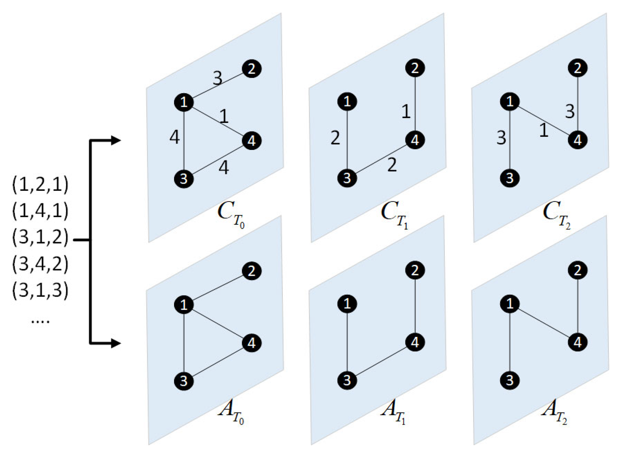
In order to better describe the details of the OESMNIE method, we construct a small temporal network for demonstration analysis, and calculate the similarity $(S_{13}^{n+1}$ or $S_{13}^{n+1})$ for nodes 1 and 3 at next period. The data preprocessing process for temporal network data is illustrated in Figure 4.

To analyze such datasets, we employ a time granularity (or time window) of length $L$ to partition the temporal network record based on the interaction timestamps ($t$). Additionally, we utilize Equations (1) and (5) to record and calculate the interaction events and fine-grained interactions of nodes in different periods. This allows us to construct the collection of snapshot matrices $A_n$ and interaction frequency matrices $C_n$.

Step 1: We utilize unweighted and weighted adjacency matrices to represent the snapshots $A_n$ and frequency matrices $C_n$, respectively. The specific expression results are shown in Figure 5.

Step 2: We use Equations (7) and (8) to calculate the probability distribution of node 1 and node 3 in each snapshot interaction frequency matrix ($C_n$). The specific calculation process in shown in Equation (14).

$$\begin{gathered} P_{T_0}\left(1,2\right)=P_{T_0}\left(2,1\right)=\frac{3}{3+4+1} \\ {P}_{T_0}\left(1,3\right)=P_{T_0}\left(3,1\right)=\frac{4}{3+4+1} \\ {P}_{T_0}\left(1,4\right)=P_{T_0}\left(4,1\right)=\frac{1}{3+4+1} \\ \cdots \\ {I}_{T_0}\left(1\right)=-\left(\frac{3}{8}\log \left(\frac{3}{8}\right)+\frac{4}{8}\log \left(\frac{4}{8}\right)+\frac{1}{8}\log \left(\frac{1}{8}\right)\right)=0.974 \\ {I}_{T_0}\left(3\right)=-\left(\frac{4}{8}\log \left(\frac{4}{8}\right)+\frac{4}{8}\log \left(\frac{4}{8}\right)\right)=0.693 \\ \begin{array}{cc}{I}_{T_1}\left(1\right)=\cdots =0& I_{T_1}\left(3\right)=\cdots =0.693\end{array} \\ \begin{array}{cc}{I}_{T_2}\left(1\right)=\cdots \approx 0.562& I_{T_2}\left(3\right)=\cdots =0\end{array} \end{gathered}$$

(14)

Node interaction entropy reflects weak ties of nodes, which plays an important role in improving the accuracy of algorithm.

Step 3: Node interaction entropy is a supplementary factor to the node’s influence within the snapshot. Therefore, in addition to incorporating the basic node structure feature, eigenvector centrality, based on the snapshot for further analysis, we also consider the calculation and combination process as shown in Equation (15).

$$\begin{gathered} E{C}_{T_0}\left(1\right)=D_{T_0}\left(1\right)={\displaystyle \sum }_j^{\tau \left(1\right)}{A}_{T_0}\left(1,j\right)\times D_{T_0}\left(j\right)=0.612 \\ E{C}_{T_0}\left(3\right)=D_{T_0}\left(3\right)={\displaystyle \sum }_j^{\tau \left(3\right)}{A}_{T_0}\left(3,j\right)\times D_{T_0}\left(j\right)=0.523 \\ \begin{array}{cc}E{C}_{T_1}\left(1\right)=D_{T_1}\left(1\right)=\cdots =0.372& E{C}_{T_1}\left(3\right)=D_{T_1}\left(3\right)=\cdots =0.602\end{array} \\ \begin{array}{cc}E{C}_{T_2}\left(1\right)=D_{T_2}\left(1\right)=\cdots =0.602& E{C}_{T_2}\left(3\right)=D_{T_2}\left(3\right)=\cdots =0.372\end{array} \\ {M}_1^{T_0}=E{C}_{T_0}\left(1\right)+I_{T_0}\left(1\right)=0.612+0.974=1.586 \\ {M}_3^{T_0}=E{C}_{T_0}\left(3\right)+I_{T_0}\left(3\right)=0.523+0.693=1.216 \\ \begin{array}{cc}{M}_1^{T_1}=\cdots =0.372& M_3^{T_1}=\cdots =1.295\end{array} \\ \begin{array}{cc}{M}_1^{T_2}=\cdots =1.164& M_3^{T_2}=\cdots =0.372\end{array} \end{gathered}$$

(15)

The first and second steps of Equation (15) involve calculating the eigenvector centrality of node 1 and node 3. Afterward, we combine it with the interaction entropy to obtain an improved node centrality. This centrality considers the node’s topology, the influence of its neighbors, and weak ties within the current snapshot. We introduce the gravity model as a tool to transform the improved node influence into node similarity. Therefore, we attempt to use the improved centrality as the mass of nodes, consider the shortest path between node 1 and node 3 as the distance, and apply the gravity model to calculate the similarity. The specific calculation is shown in Equation (16).

$$\begin{gathered} C_{\left(1,3\right)}^{T_0}=\frac{M_1^{T_0}\times M_3^{T_0}}{{(d_{\left(1,3\right)}^{T_0})}^2}=\frac{1.586\times 1.216}{{(1)}^2}=1.929\\ \\ {C}_{\left(1,3\right)}^{T_1}=\frac{M_1^{T_1}\times M_3^{T_1}}{{(d_{\left(1,3\right)}^{T_1})}^2}=\frac{0.372\times 1.295}{{(1)}^2}=0.963\\ \\ {C}_{\left(1,3\right)}^{T_2}=\frac{M_1^{T_2}\times M_3^{T_2}}{{(d_{\left(1,3\right)}^{T_2})}^2}=\frac{1.164\times 0.372}{{(1)}^2}=0.433 \end{gathered}$$

(16)

Step 4: We start by calculating the sum of node interaction entropy for each snapshot. Among these values, we select the snapshot with the maximum sum of node interaction entropy as the denominator, while using the sum of node interaction entropy for each snapshot as the numerator. Next, we combine this ratio with the smoothing coefficient $\alpha$ to dynamically control its impact on the prediction process, ensuring its practical influence on the predicted results. The smoothing coefficient $\alpha$ is a variable parameter, and we set it to 0.5 in this case. For a traditional exponential smoothing model, this implies that the recent node similarity information will be assigned a reference weight of 0.5, while the remaining 0.5 reference value will serve as the reference weight for the historical node similarity after compression iteration. The actual reference proportion of node similarity matrices in the exponential smoothing model can be calculated using the method described in Equation (17).

$$\begin{gathered} W_{T_0}=\frac{{{\displaystyle \sum }}_i^{V(A_{T_0})}{I}_{T_0}\left(i\right)}{Max(T\in \left[T_0,T_1,T_2\right]|{{\displaystyle \sum }}_i^{V(A_{T_0})}{I}_T\left(i\right))}·\alpha =\frac{2.168}{2.168}\alpha =\frac{2.168}{2.168}·0.5=0.5 \\ {W}_{T_1}=\frac{{{\displaystyle \sum }}_i^{V(A_{T_1})}{I}_{T_1}\left(i\right)}{Max(T\in \left[T_0,T_1,T_2\right]|{{\displaystyle \sum }}_i^{V(A_{T_0})}{I}_T\left(i\right))}·\alpha =\frac{1.329}{2.168}\alpha =\frac{1.329}{2.168}·0.5=0.3075 \\ {W}_{T_2}=\frac{{{\displaystyle \sum }}_i^{V(A_{T_2})}{I}_{T_2}\left(i\right)}{Max(T\in \left[T_0,T_1,T_2\right]|{{\displaystyle \sum }}_i^{V(A_{T_0})}{I}_T\left(i\right))}·\alpha =\frac{1.125}{2.168}·\alpha =\frac{1.125}{2.168}·0.5=0.2595 \end{gathered}$$

(17)

Step 5: After determining the reference ratio of node similarity values in different periods, we can substitute the parameters into the exponential smoothing model to predict the similarity sequence between node 1 and node 3 in $T_3$ period. The specific prediction process is shown in Equation (18).

$$\begin{array}{c}{S}_{13}^1=C_{\left(1,3\right)}^{T_0}=1.929\\ S_{13}^2=W_{T_1}·C_{\left(1,3\right)}^{T_1}+\left(1-W_{T_1}\right)·S_{13}^1=0.3065·0.963+0.6935·1.929=1.633\\ S_{13}^3=W_{T_2}·C_{\left(1,3\right)}^{T_2}+\left(1-W_{T_2}\right)·S_{13}^2=0.2595·0.433+0.7405·1.633=1.3216\end{array}$$

(18)

where, $S_{13}^3$ is the node similarity between node 1 and node 3 in the future network snapshot $A_{T_3}$. We consider it as the prediction score for the link.

4. Experiments and Discussion

4.1. Experimental Environment

The experimental environment for this study is as follows: Processor: 12th Gen Intel (R) Core (TM) i5-12400F 2.50GHz; Memory: 16.0 GB (DDR4); Operating system: Windows 11 Professional (22H2); Compiler version: Python 3.7; and Relevant tool libraries: NetworkX 2.3, Numpy 1.21.6, and Multinetx.

4.2. Data Selection

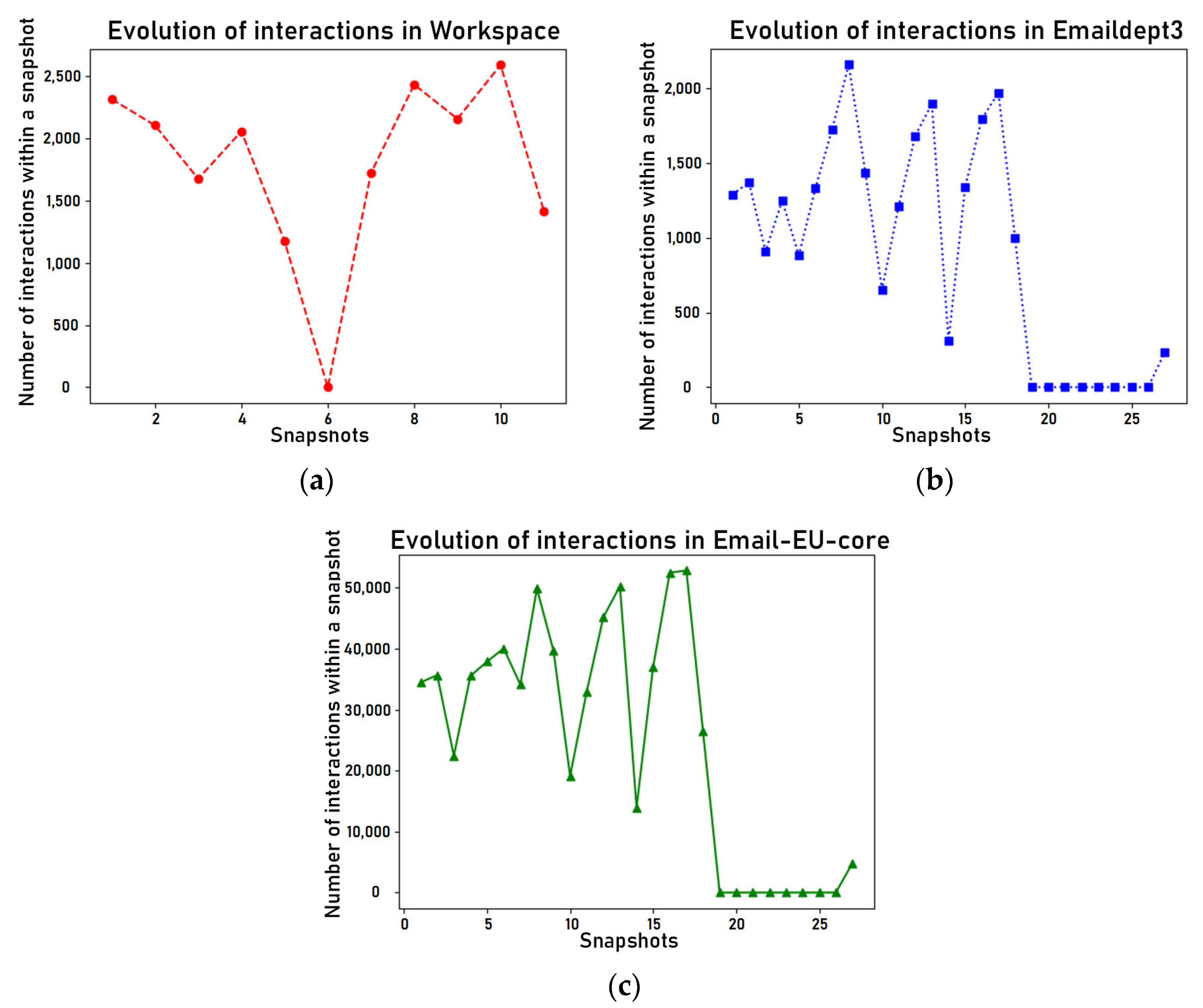
We selected three real temporal network datasets, including Emaildept3 [44], Workspace [45], and Email-EU-core [46], to verify the efficiency and accuracy of the OESMNIE method and compare it with TBNS, GR, and traditional node similarity indicators.

Table 2. Description of datasets.

Data Set 1	N	C	Span
Workspace	92	9287	6/24–7/3, 2013
Emaildept3	89	12,216	802 days
Email-EU-core	986	332,334	803 days

Note: ¹ The selected temporal network datasets possess the following characteristics: Firstly, they are medium-sized or small-sized networks, providing practical storage conditions for the matrix-based representation of snapshots in the proposed method. Secondly, they encompass both short-term and long-term temporal interaction information, which help demonstrate the compatibility of the OESMNIE method in the temporal dimension. Lastly, they exhibit significant fluctuations in interactions (including periods of no interactions), which accurately reflect the dynamic nature of real-world networks. This contributes to validating the rationality of the dynamic weighting approach in the prediction process and the reliability of the OESMNIE method; N is the number of nodes in the temporal network, and C is the actual number of interactions that occurred during the observation period; In the above temporal network, the connections are recorded in the form of triplets $\left(i,j,t\right)$, where $t$ is in seconds.

shows the statistical characteristics of the selected temporal network datasets. Figure 6 illustrates the evolution of snapshot interactions in each temporal network dataset.

To validate the effectiveness of the OESMNIE method under different time granularities, we utilize different time granularities to obtain snapshots. The number of network snapshots generated based on the time granularity $L$ is represented in

Table 3. Number of temporal network snapshots.

Data Set	$\mathit{L}$	T
Workspace	1 day	10
Workspace	2 days	5
Emaildept3	7 days	115
Emaildept3	30 days	27
Emaildept3	120 days	7
Email-EU-core	7 days	115
Email-EU-core	30 days	27
Email-EU-core	120 days	7

Note: $L$ is the time granularity used to partition the temporal network, which can also be understood as the span of a single network snapshot; and T is the number of network snapshots.

.

4.3. Evaluation Method

We validate the algorithm from two perspectives. First, we predict the individual snapshots in the temporal network (which serves to verify the effectiveness of fine-grained interaction behavior among nodes in improving node similarity). Second, we predict the future links of the temporal network (which serves to verify the effectiveness of dynamically adjusting the smoothing coefficient based on the temporal network’s interaction changes in link prediction). We treat the individual snapshot $A_n$ (randomly selected from the snapshot set of the temporal network) as a static network. We divide the edges within snapshot $A_n$ into training data $E_{tr}$ and testing data $E_{te}$ in a ratio of 20%. Therefore, the set $E^{\prime }$ consists of edges that do not actually exist in the snapshot (constructed as $E^{\prime }=U_n-E_{tr}-E_{te}$). We divide the snapshot set into training and test datasets for future prediction (based on all network snapshots). Assuming that the graph data represented by the snapshot set of the temporal network is $G=\left(V,E\right)$, since $G$ is composed of snapshots from different periods, the snapshot subgraphs contained in $G$ can be denoted as $G=\left\{G_0, G_1,\cdots ,G_n\right\}$, and the corresponding edge and node dataset can be represented by $G_T=\left(V_T,E_T\right)$. Therefore, we take the subset $G$ of elements $G_0$ to $G_{n-1}$ from the set $G$ as the training data $E_{tr}$, including {$E_0,E_1,\cdots ,E_{n-1}$}. In order to predict the link status of the next snapshot, we set the edge set $E_n$ of the $G_n$ subgraph (i.e., the latest snapshot) as the test dataset $E_{te}$. We use the AUC to evaluate the prediction performance of individual snapshots and the entire temporal network at future. The definition of the AUC is given in Equation (19).

$$AUC=\frac{n^{\prime }+0.5n^{\prime \prime }}{n}$$

(19)

The AUC randomly selects pairs of edges, one from the dataset of actual existing edges $E_{te}$, and another from the dataset of actual non-existing edges $E^{\prime }$, and compares their predicted score multiple times. $n^{\prime }$ is the number of times that the predicted score of an actual existing edge is greater than an actual non-existing edge in experiments. $n^{″}$ is the number of times that the predicted score of an actual existing edge is equal to an actual non-existing edge. $n$ is the total number of selections in the validation experiments. The value of the AUC indicator will range between 0.5 and 1, and the closer it is to 1, the more accurate is the method’s prediction.

4.4. Performance Comparison

Firstly, we compared the AUC of our proposed method with the existing GR, CN, AA, JC, PA, and RA indictors on a single snapshot with different time granularities. These selected indicators are based on local information to construct the similarity between nodes and have been widely applied in link prediction. Therefore, they are similar to the OESMNIE method in terms of the topological structure and are representative of the field. The results are presented in

Table 4. AUC of OESMNIE and other indicators comparison.

Data Set	$\mathit{L}$	OESMNIE	GR	CN	AA	JC	PA	RA
Workspace	1	0.8772	0.7229	0.7219	0.7254	0.7010	0.7348	0.7249
Workspace	2	0.8928	0.7300	0.7213	0.7284	0.7661	0.6730	0.7264
Email-EU-core	7	0.8856	0.7898	0.7457	0.7327	0.7620	0.8717	0.7787
Email-EU-core	30	0.9118	0.8676	0.8683	0.8438	0.8654	0.874	0.8741
Email-EU-core	120	0.9148	0.9063	0.9287	0.8932	0.9235	0.8837	0.9353

.

In Table 4, our proposed OESMNIE method demonstrates competitive performance across single-layer snapshots of temporal networks at varying time granularities. As the temporal granularity L increases, all link prediction methods based on local information show improved accuracy. This can be attributed to the fact that a larger time granularity L allows for capturing more interaction information within the snapshot, thereby enhancing the information richness of the snapshot. However, for temporal network link prediction, increasing the temporal granularity disrupts the temporal attributes of node interaction information, thus hindering future link prediction. In contrast, the OESMNIE method leverages the fine-grained interactions of the current snapshot and exploits the weak ties between nodes, resulting in a significant improvement in accuracy while maintaining the same snapshot conditions. This approach neither compromises the snapshot’s temporal features nor their ability to characterize the node similarity across snapshots accurately.

Secondly, we conducted 100 experiments and averaged the results to compare the predictive performance of the OESMNIE method with selected time series-based temporal link prediction methods. Figure 7 illustrates the AUC results of these eight methods on the temporal network.

In the temporal network with weekly and monthly time granularities, the OESMNIE method outperforms other methods, achieving the highest scores of 0.9181 and 0.9384, respectively. The other methods show a significant decrease in accuracy under different time granularities. Two factors cause the decreased accuracy of these methods. First, the node similarity matrix is constructed based on limited adjacency matrix information from the network snapshots, and thus limiting the accuracy of node similarity within a single snapshot. Second, relying on the attenuation constant of the GR or using the exponential smoothing model can cause the algorithm to deviate from the actual network interactions during the prediction process, leading to other methods providing incorrect reference scores at the wrong snapshot period.

4.5. Parameters Analysis

The time granularity $L$ used to construct network snapshots is a critical factor influencing the performance of the temporal network link prediction methods. In addition, we also consider that the smoothing coefficient $\alpha$ in the improved exponential smoothing model plays an important role on the algorithm’s accuracy. Therefore, we explored the impact of the smoothing coefficient on the algorithm’s effectiveness by incrementally varying $\alpha$. Based on the network snapshots with different time granularities for different networks, we can observe the relationship between the change in the number of interactions within each snapshot and the smoothing coefficient $\alpha$’s ($\alpha =0.8$) reference ratio, as shown in Figure 8, Figure 9 and Figure 10.

From Figure 8, Figure 9 and Figure 10, we can observe that the smoothing coefficient in the exponential smoothing model varies and adjusts with the interaction patterns within the snapshots. This provides more moderate weights for the predicted node similarity values. The experimental results are consistent with our initial hypothesis.

To further determine the impact of the smoothing coefficient $\alpha$ on the prediction accuracy of the OEMSNIE method, we conduct a comparative analysis with similar methods for varying $\alpha$ values. Figure 11, Figure 12 and Figure 13 shows the detailed comparison results.

As shown in Figure 11 and Figure 12, prediction accuracy fluctuations are observed for all algorithms with the increase in the smoothing coefficient $\alpha$ and the snapshot time granularity $L$. However, the OESMNIE method demonstrates overall stability, indicating its superior stability to the other algorithms. This further validates the improved prediction weights’ effectiveness in adapting to network structure changes.

As shown in Figure 13a, the accuracy of the OESMNIE method is weaker than other indicators, but this is only limited to the case of a small snapshot period. From the overall experimental results, the method proposed in this paper shows better robustness and accuracy than other methods under different time granularities and smoothing coefficients.

4.6. Discussion

Although our proposed method has achieved certain results, it is essential to acknowledge its limitations. Firstly, our approach focuses on extracting more link information from the snapshot to establish the similarity between nodes within each period, which is used for link prediction. As a result, the structure of each snapshot is represented in a matrix. However, for large networks, the data processing approach based on the adjacency matrix of network snapshots can result in larger sparse matrices, thereby increasing storage burden. Hence, it is more suitable for small-sized and medium-sized networks. Secondly, in constructing node similarity, we use the shortest path length between nodes as the distance in the gravity model. Therefore, the node similarity matrices are symmetric, indicating that the current method only applies to unweighted and undirected temporal networks. Finally, the OESMNIE algorithm requires snapshots to contain fine-grained interaction information among nodes to distinguish the similarity between nodes. Therefore, when dealing with real-time link prediction, the OESMNIE method can only record the real-time data and transform it into a near real-time approach for prediction. In future research, we can explore graph embedding techniques to alleviate the sparsity issue in large networks and improve the measurement of node similarity to make the method applicable to a wider range of network types and application scenarios.

5. Conclusions

In this paper, we propose a temporal network link prediction method based on network snapshots, which addresses the problems of insufficient information in snapshot representations and the continuity of connection time information which is easily destroyed by the multi-layer network model. We conduct experiments on single and overall network snapshots with different time granularities. The experimental results verify that the OESMNIE method outperforms its counterparts in time series-based temporal link prediction based on the local similarity of nodes. Subsequently, we analyzed the effects of the smoothing coefficient and the time granularity on the prediction, validating the effectiveness of the weights in changing with the variations in the snapshot structure. Finally, we comprehensively compared the AUC metric, snapshot time granularity, and exponential smoothing coefficient. This comparison confirmed the stability and robustness of our method. In conclusion, our approach can effectively predict future linkages within the given periods.

References

1. Lü, L.; Zhou, T. Link prediction in complex networks: A survey. Phys. A Stat. Mech. Its Appl. 2011, 390, 1150–1170. [Google Scholar] [CrossRef]
2. Abbas, K.; Abbasi, A.; Dong, S.; Niu, L.; Yu, L.; Chen, B.; Cai, S.-M.; Hasan, Q. Application of network link prediction in drug discovery. BMC Bioinform. 2021, 22, 1–21. [Google Scholar] [CrossRef] [PubMed]
3. Symeonidis, P.; Iakovidou, N.; Mantas, N.; Manolopoulos, Y. From biological to social networks: Link prediction based on multi-way spectral clustering. Data Knowl. Eng. 2013, 87, 226–242. [Google Scholar] [CrossRef]
4. Cannistraci, C.V.; Alanis-Lobato, G.; Ravasi, T. From link-prediction in brain connectomes and protein interactomes to the local-community-paradigm in complex networks. Sci. Rep. 2013, 3, 1613. [Google Scholar] [CrossRef] [PubMed]
5. Bocu, R.; Bocu, D.; Iavich, M. Objects Detection Using Sensors Data Fusion in Autonomous Driving Scenarios. Electronics 2021, 10, 2903. [Google Scholar] [CrossRef]
6. Liu, R.; Zhang, S.; Zhang, D.; Zhang, X.; Bao, X. Node Importance Identification for Temporal Networks Based on Optimized Supra-Adjacency Matrix. Entropy 2022, 24, 1391. [Google Scholar] [CrossRef]
7. Wen, T.; Cheong, K.H. The fractal dimension of complex networks: A review. Inf. Fusion 2021, 73, 87–102. [Google Scholar] [CrossRef]
8. Fortunato, S. Community detection in graphs. Phys. Rep. 2010, 486, 75–174. [Google Scholar] [CrossRef]
9. Liu, H. Using link prediction to predict network evolution mechanism. Sci. Sin. Phys. Mech. Astron. 2011, 41, 816–823. [Google Scholar]
10. Kaya, B. A hotel recommendation system based on customer location: A link prediction approach. Multimed. Tools Appl. 2020, 79, 1745–1758. [Google Scholar] [CrossRef]
11. Si, S.; Wang, J.; Yu, C.; Zhao, H. Energy-efficient and fault-tolerant evolution models based on link prediction for large-scale wireless sensor networks. IEEE Access 2018, 6, 73341–73356. [Google Scholar] [CrossRef]
12. Poleksic, A. Hyperbolic matrix factorization improves prediction of drug-target associations. Sci. Rep. 2023, 13, 959. [Google Scholar] [CrossRef] [PubMed]
13. Divakaran, A.; Mohan, A. Temporal Link Prediction: A Survey. New Gener. Comput. 2019, 38, 213–258. [Google Scholar] [CrossRef]
14. Gao, S.; Denoyer, L.; Gallinari, P. Temporal link prediction by integrating content and structure information. In Proceedings of the 20th ACM International Conference on Information and Knowledge Management, Arlington, VA, USA, 11 November 2011; pp. 1169–1174. [Google Scholar]
15. Ouzienko, V.; Guo, Y.; Obradovic, Z. Prediction of attributes and links in temporal social networks. In ECAI 2010; IOS Press: Washington, DC, USA, 2010; pp. 1121–1122. [Google Scholar]
16. Zhou, L.; Yang, Y.; Ren, X.; Wu, F.; Zhuang, Y. Dynamic network embedding by modeling triadic closure process. In Proceedings of the AAAI Conference on Artificial intelligence, New Orleans, LA, USA, 2–7 February 2018. [Google Scholar]
17. Huang, X.; Chen, D.; Ren, T. A Feasible Temporal Links Prediction Framework Combining with Improved Gravity Model. Symmetry 2020, 12, 100. [Google Scholar] [CrossRef]
18. Yang, X.; Tian, Z.; Cui, H.; Zhang, Z. Link prediction on evolving network using tensor-based node similarity. In Proceedings of the 2012 IEEE 2nd International Conference on Cloud Computing and Intelligence Systems, Hangzhou, China, 30 October–1 November 2012; IEEE: Piscataway, NJ, USA, 2012; pp. 154–158. [Google Scholar]
19. Güneş, İ.; Gündüz-Öğüdücü, Ş.; Çataltepe, Z. Link prediction using time series of neighborhood-based node similarity scores. Data Min. Knowl. Discov. 2016, 30, 147–180. [Google Scholar] [CrossRef]
20. Lorrain, F.; White, H.C. Structural equivalence of individuals in social networks. J. Math. Sociol. 1971, 1, 49–80. [Google Scholar] [CrossRef]
21. Etude, P.J. comparative de la distribution florale dans une portion des Alpes et des Jura. Bull. Soc. Vaud. Sci. Nat 1901, 37, 547. [Google Scholar]
22. Ravasz, E.; Somera, A.L.; Mongru, D.A.; Oltvai, Z.N.; Barabási, A.-L. Hierarchical organization of modularity in metabolic networks. Science 2002, 297, 1551–1555. [Google Scholar] [CrossRef]
23. Molloy, M.; Reed, B. A critical point for random graphs with a given degree sequence. Random Struct. Algorithms 1995, 6, 161–180. [Google Scholar] [CrossRef]
24. Adamic, L.A.; Adar, E. Friends and neighbors on the web. Soc. Netw. 2003, 25, 211–230. [Google Scholar] [CrossRef]
25. Zhou, T.; Lü, L.; Zhang, Y.-C. Predicting missing links via local information. Eur. Phys. J. B 2009, 71, 623–630. [Google Scholar] [CrossRef]
26. Barabási, A.-L.; Albert, R. Emergence of scaling in random networks. Science 1999, 286, 509–512. [Google Scholar] [CrossRef] [PubMed]
27. Lü, L.; Jin, C.-H.; Zhou, T. Similarity index based on local paths for link prediction of complex networks. Phys. Rev. E 2009, 80, 046122. [Google Scholar] [CrossRef] [PubMed]
28. Liu, W.; Lü, L. Link prediction based on local random walk. Europhys. Lett. 2010, 89, 58007. [Google Scholar] [CrossRef]
29. Fouss, F.; Pirotte, A.; Renders, J.-M.; Saerens, M. Random-walk computation of similarities between nodes of a graph with application to collaborative recommendation. IEEE Trans. Knowl. Data Eng. 2007, 19, 355–369. [Google Scholar] [CrossRef]
30. Klein, D.J.; Randić, M. Resistance distance. J. Math. Chem. 1993, 12, 81–95. [Google Scholar] [CrossRef]
31. Liu, M.; Tu, Z.; Su, T.; Wang, X.; Xu, X.; Wang, Z. BehaviorNet: A Fine-grained Behavior-aware Network for Dynamic Link Prediction. ACM Transactions on the web. 2023. [CrossRef]
32. Taylor, D.; Myers, S.A.; Clauset, A.; Porter, M.A.; Mucha, P.J. Eigenvector-Based Centrality Measures for Temporal Networks. Multiscale Model. Simul. 2017, 15, 537–574. [Google Scholar] [CrossRef]
33. Granovetter, M.S. The strength of weak ties. Am. J. Sociol. 1973, 78, 1360–1380. [Google Scholar] [CrossRef]
34. Borgatti, S.P.; Halgin, D.S. On network theory. Organ. Sci. 2011, 22, 1168–1181. [Google Scholar] [CrossRef]
35. Lü, L.; Zhou, T. Role of weak ties in link prediction of complex networks. In Proceedings of the 1st ACM International Workshop on Complex Networks Meet Information & Knowledge Management, Hong Kong, China, 2–6 November 2009; pp. 55–58. [Google Scholar]
36. Levy, M.; Goldenberg, J. The gravitational law of social interaction. Phys. A Stat. Mech. Its Appl. 2014, 393, 418–426. [Google Scholar] [CrossRef]
37. Wahid-Ul-Ashraf, A.; Budka, M.; Musial, K. How to predict social relationships—Physics-inspired approach to link prediction. Phys. A Stat. Mech. Its Appl. 2019, 523, 1110–1129. [Google Scholar] [CrossRef]
38. Xu, Z.; Pu, C.; Yang, J. Link prediction based on path entropy. Phys. A Stat. Mech. Its Appl. 2016, 456, 294–301. [Google Scholar] [CrossRef]
39. Xu, H.; Luo, R.; Winnink, J.; Wang, C.; Elahi, E. A methodology for identifying breakthrough topics using structural entropy. Inf. Process. Manag. 2022, 59, 102862. [Google Scholar] [CrossRef]
40. Yuyu, M.; Jing, G. Link prediction algorithm based on node structure similarity measured by relative entropy. In Journal of Physics: Conference Series; IOP Publishing: Bristol, UK, 2021; p. 012078. [Google Scholar]
41. Baltakiene, M.; Baltakys, K.; Cardamone, D.; Parisi, F.; Radicioni, T.; Torricelli, M.; de Jeude, J.; Saracco, F. Maximum entropy approach to link prediction in bipartite networks. arXiv 2018, arXiv:1805.04307. [Google Scholar]
42. Bonacich, P. Factoring and Weighing Approaches to Clique Identification. J. Math. Sociol. 1971, 92, 1170–1182. [Google Scholar]
43. Huang, Z.; Lin, D.K. The time-series link prediction problem with applications in communication surveillance. Inf. J. Comput. 2009, 21, 286–303. [Google Scholar] [CrossRef]
44. Erkol, Ş.; Mazzilli, D.; Radicchi, F. Influence maximization on temporal networks. Phys. Rev. E 2020, 102, 042307. [Google Scholar] [CrossRef]
45. Génois, M.; Vestergaard, C.L.; Fournet, J.; Panisson, A.; Bonmarin, I.; Barrat, A. Data on face-to-face contacts in an office building suggest a low-cost vaccination strategy based on community linkers. Netw. Sci. 2015, 3, 326–347. [Google Scholar] [CrossRef]
46. Paranjape, A.; Benson, A.R.; Leskovec, J. Motifs in temporal networks. In Proceedings of the Tenth ACM International Conference on Web Search and Data Mining, Cambridge, UK, 6–10 February 2017; pp. 601–610. [Google Scholar]
Figure 1. Temporal network link prediction based on time-series.
Symmetry 15 01182 g001
Figure 2. (a) Visualization examples of adjacency matrices (network snapshots) using the SAM model; (b) Visualization of the network structure constructed from the network snapshots in (a).
Symmetry 15 01182 g002
Figure 3. Framework of the OSMNIE method.
Symmetry 15 01182 g003
Figure 4. Example temporal network. Temporal network datasets are commonly represented as triples i ,   j ,   t , where i represents the source node, j represents the target node, and t represents the interaction timestamp.
Symmetry 15 01182 g004
Figure 5. Matrix representation of C n and A n . The edge weight of the snapshot interaction frequency matrix C n is the total number of connections generated by the above nodes in the corresponding snapshot inclusion period. The network snapshot A n indicates that each node has a connection event in the corresponding period.
Symmetry 15 01182 g005
Figure 6. (a) Temporal evolution of workspace interactions; (b) Temporal evolution of Emaildept3 interactions; (c) Temporal evolution of Email-EU-core interactions.
Symmetry 15 01182 g006
Figure 7. (a) The comparison results of various methods when the time granularity for generating snapshots in week. (b) The comparison results of various methods when the time granularity for generating snapshots in month.
Symmetry 15 01182 g007
Figure 8. (a) The graph describes the relationship between the sum of interactions of daily snapshots generated in the Workspace network and the reference score. (b) The graph depicts the relationship between the sum of interactions of snapshots generated in the Workspace network with a time granularity of two days and the reference score.
Symmetry 15 01182 g008
Figure 9. (a) The graph describes the relationship between the sum of interactions of weekly snapshots generated in the Emaildept3 network and the reference score. (b) The graph depicts the relationship between the sum of interactions of snapshots generated in the Emaildept3 network with a time granularity of month and the reference score. (c) The graph depicts the relationship between the sum of interactions of snapshots generated in the Emaildept3 network with a time granularity of quarter and the reference score.
Symmetry 15 01182 g009
Figure 10. (a) The graph describes the relationship between the sum of interactions of weekly snapshots generated in the Email-EU-core network and the reference score. (b) The graph depicts the relationship between the sum of interactions of snapshots generated in the Email-EU-core network with a time granularity of month and the reference score. (c) The graph depicts the relationship between the sum of interactions of snapshots generated in the Email-EU-core network with a time granularity of quarter and the reference score.
Symmetry 15 01182 g010
Figure 11. Comparison of various methods on the Workspace network. (a) The AUC scores of various methods under different smoothing coefficients are evaluated when the time granularity in the Workspace network is 1 day. (b) The AUC scores of various methods under different smoothing coefficients are evaluated when the time granularity in the Workspace network is 2 days.
Symmetry 15 01182 g011aSymmetry 15 01182 g011b
Figure 12. Comparison of various methods on the Emaildept3 network. (a) The AUC scores of various methods under different smoothing coefficients are evaluated when the time granularity in the Emaildept3 network is 7 days. (b) The AUC scores of various methods under different smoothing coefficients are evaluated when the time granularity in the Emaildept3 network is 30 days. (c) The AUC scores of various methods under different smoothing coefficients are evaluated when the time granularity in the Emaildept3 network is 120 days.
Symmetry 15 01182 g012aSymmetry 15 01182 g012b
Figure 13. Comparison of various methods on the Email-EU-core network. (a) The AUC scores of various methods under different smoothing coefficients are evaluated when the time granularity in the Email-EU-core network is 7 days. (b) The AUC scores of various methods under different smoothing coefficients are evaluated when the time granularity in the Email-EU-core network is 30 days. (c) The AUC scores of various methods under different smoothing coefficients are evaluated when the time granularity in the Email-EU-core network is 120 days.
Symmetry 15 01182 g013aSymmetry 15 01182 g013b