
Calibration Estimation of Cumulative Distribution Function Using Robust Measures

 , , ,
, , ,
Abstract
1. Introduction
2. First Adapted Calibration Estimator of CDF Using Robust Measure
2.1. First Adapted Calibration Estimator of CDF
2.2. Second Adapted Calibration Estimator of CDF
3. Proposed Estimator
3.1. First Proposed Calibration Estimator of CDF
3.2. Second Proposed Calibration Estimator of CDF
4. Numerical Study
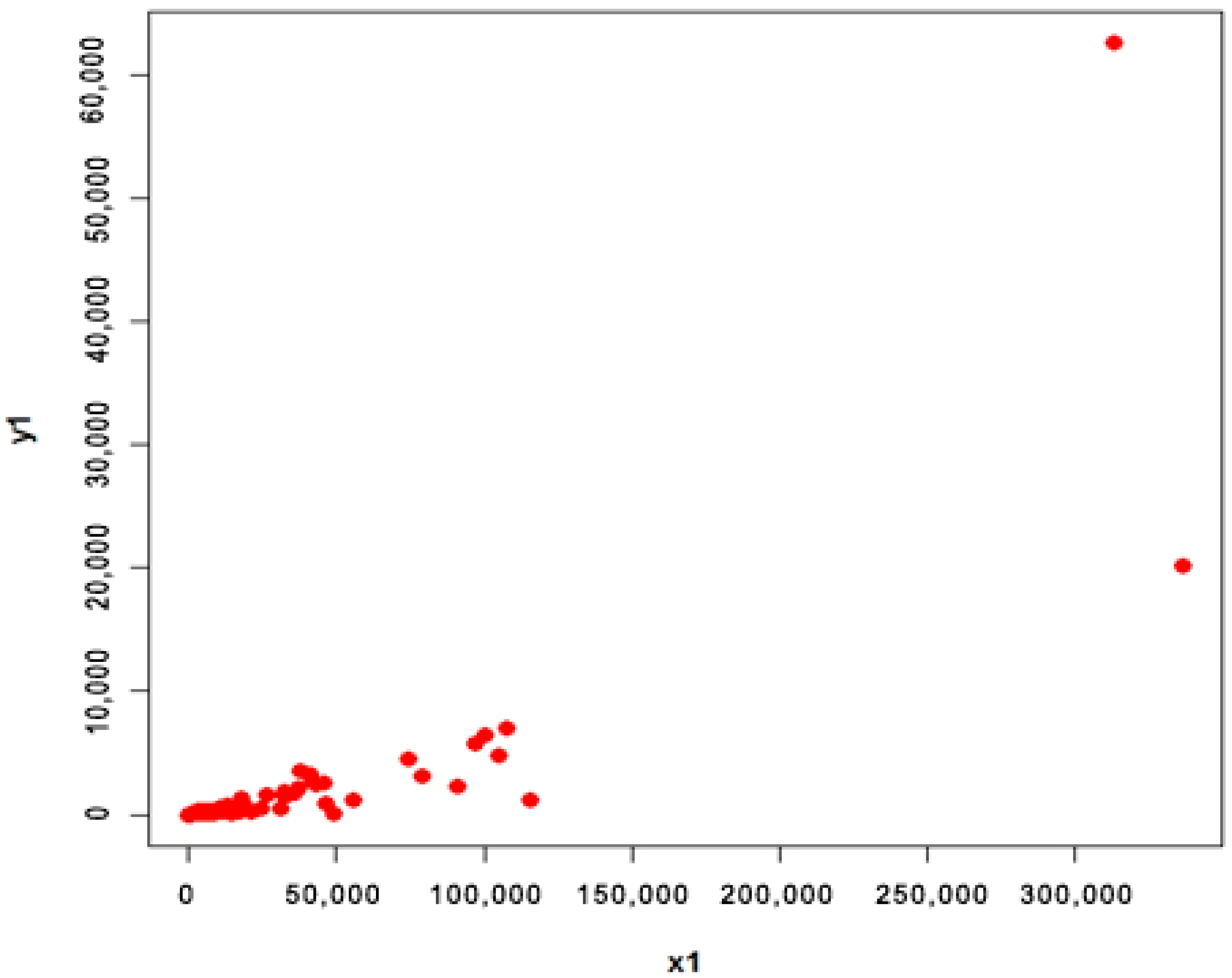
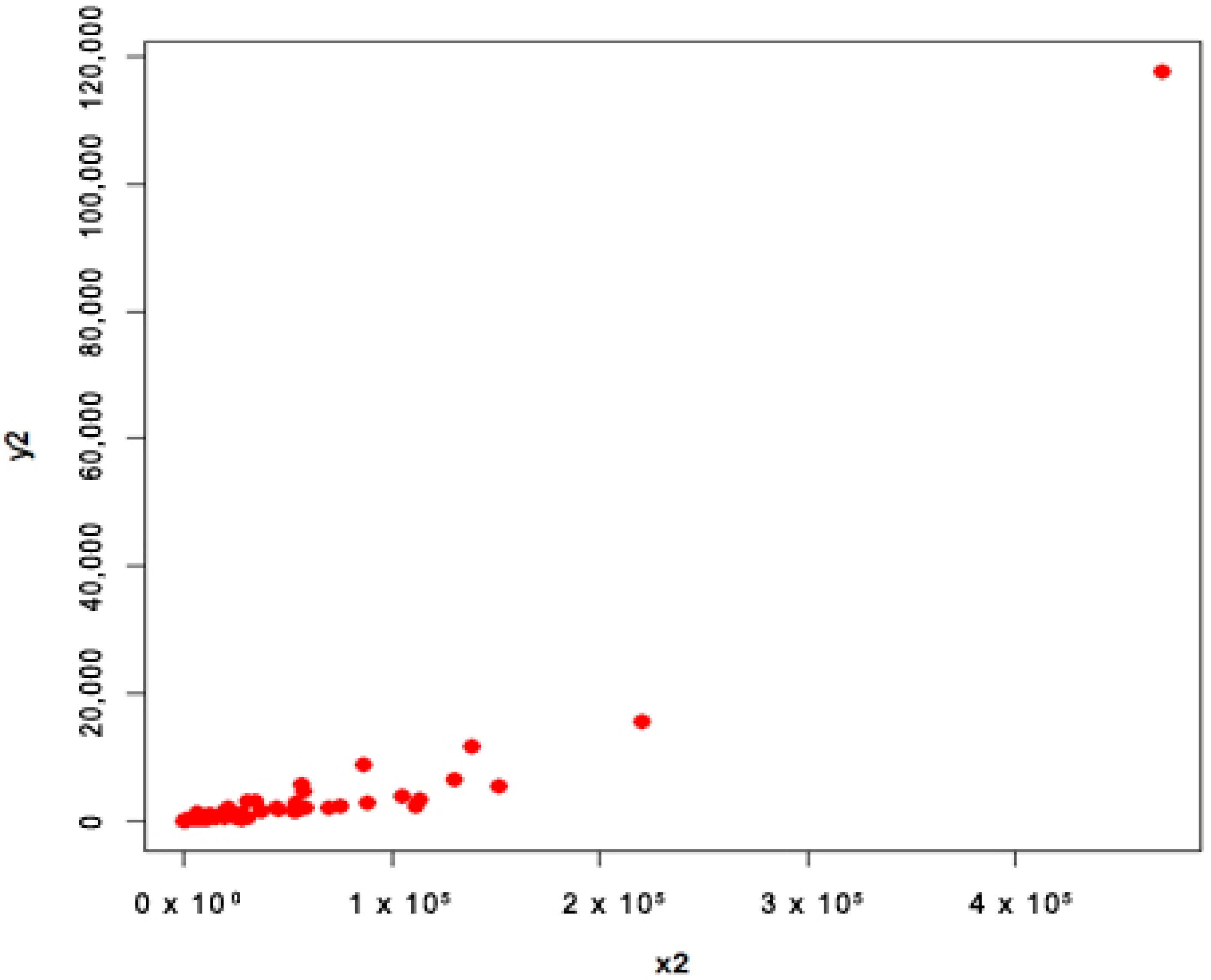
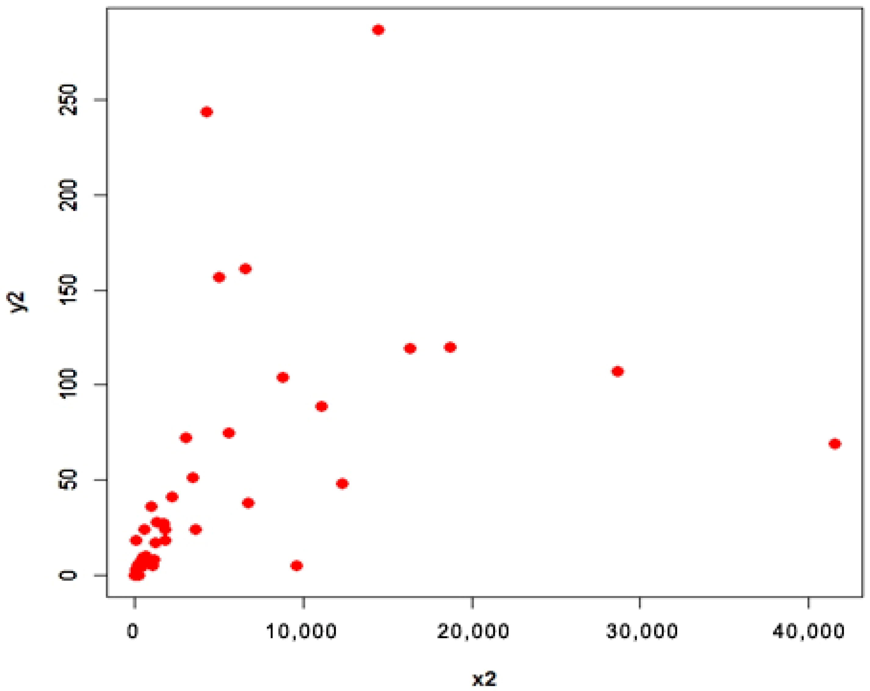
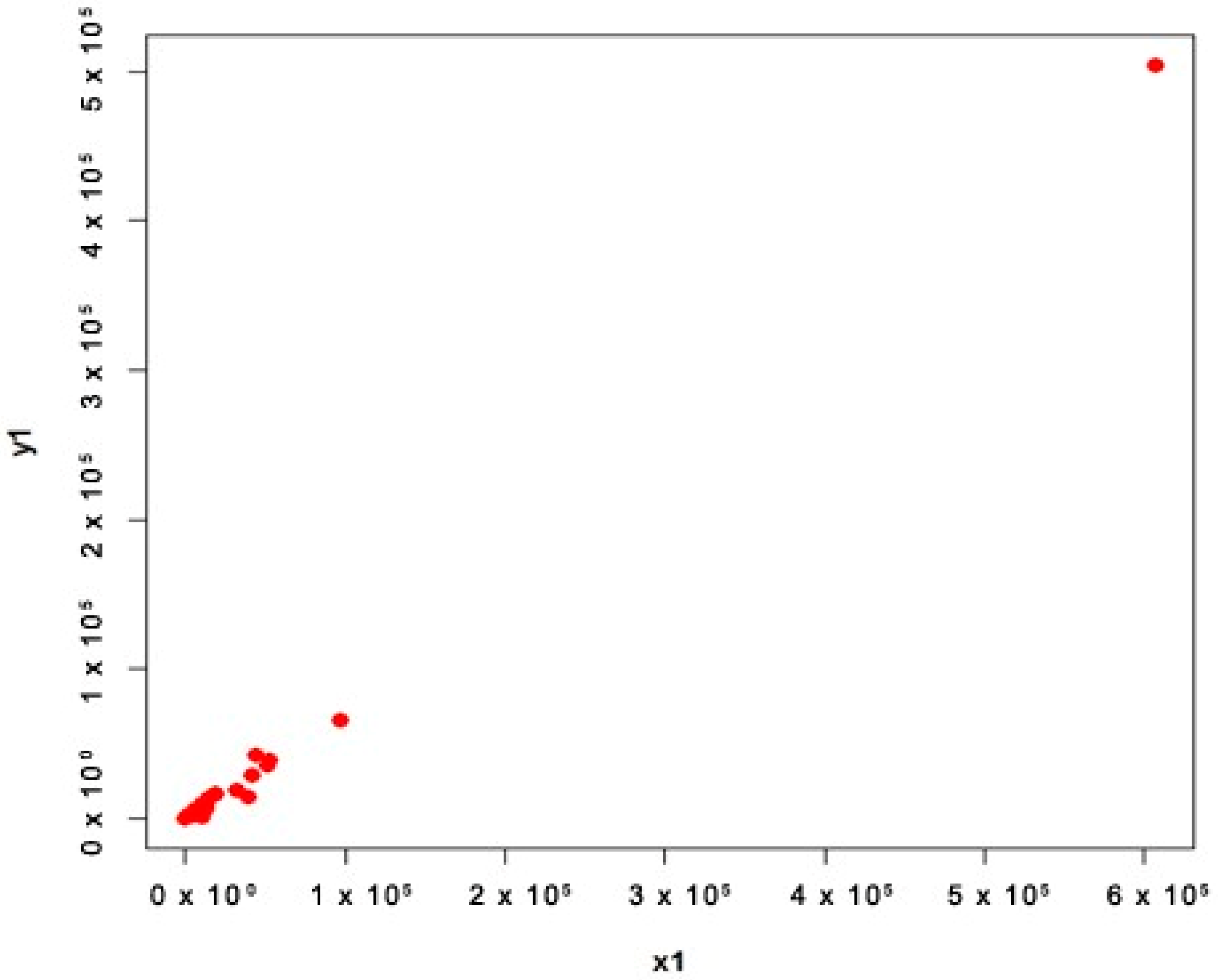
4.1. Apple Data (Population 1 and 2)
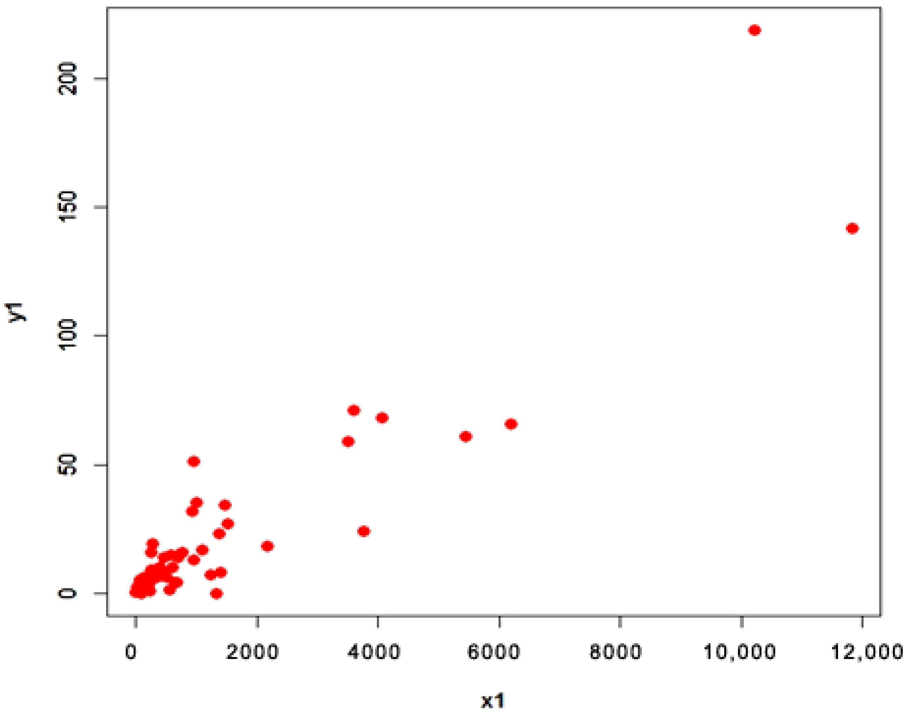
- Population 1
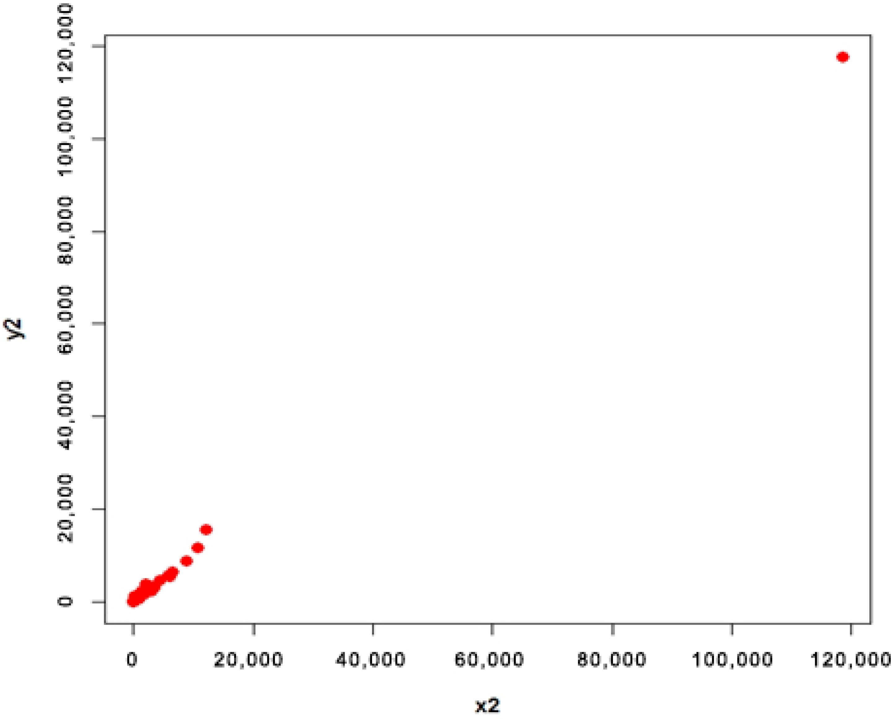
- Population 2
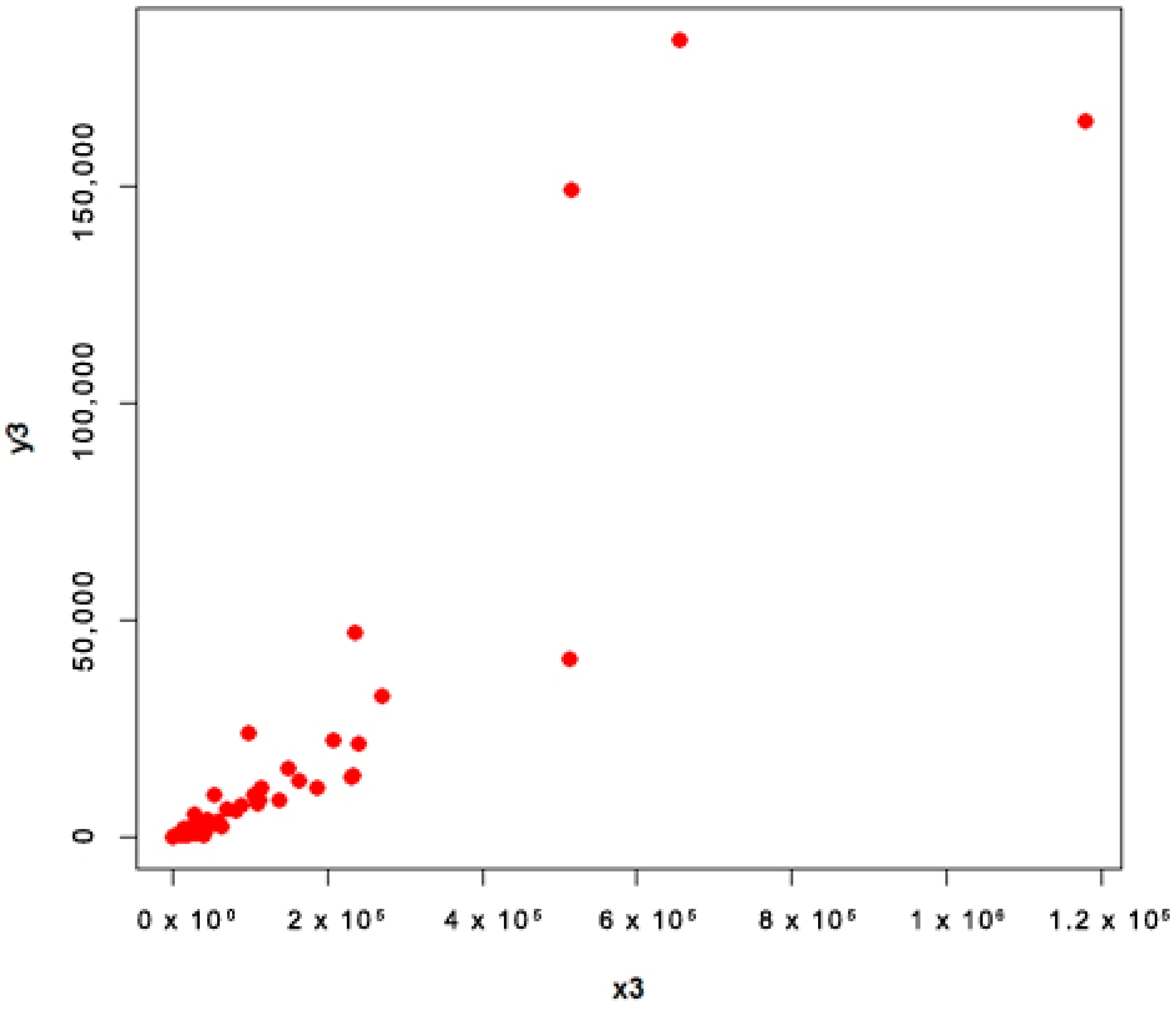
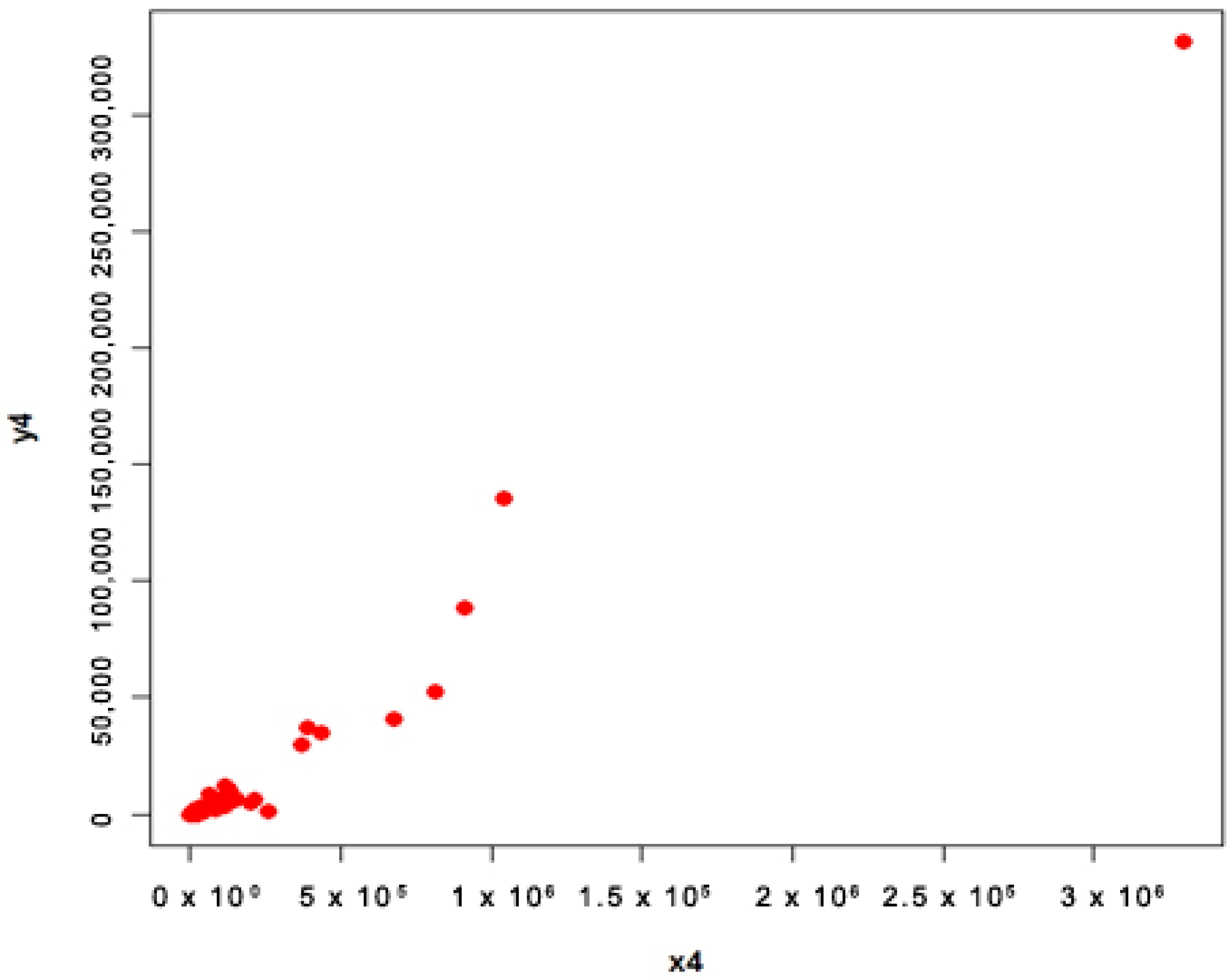
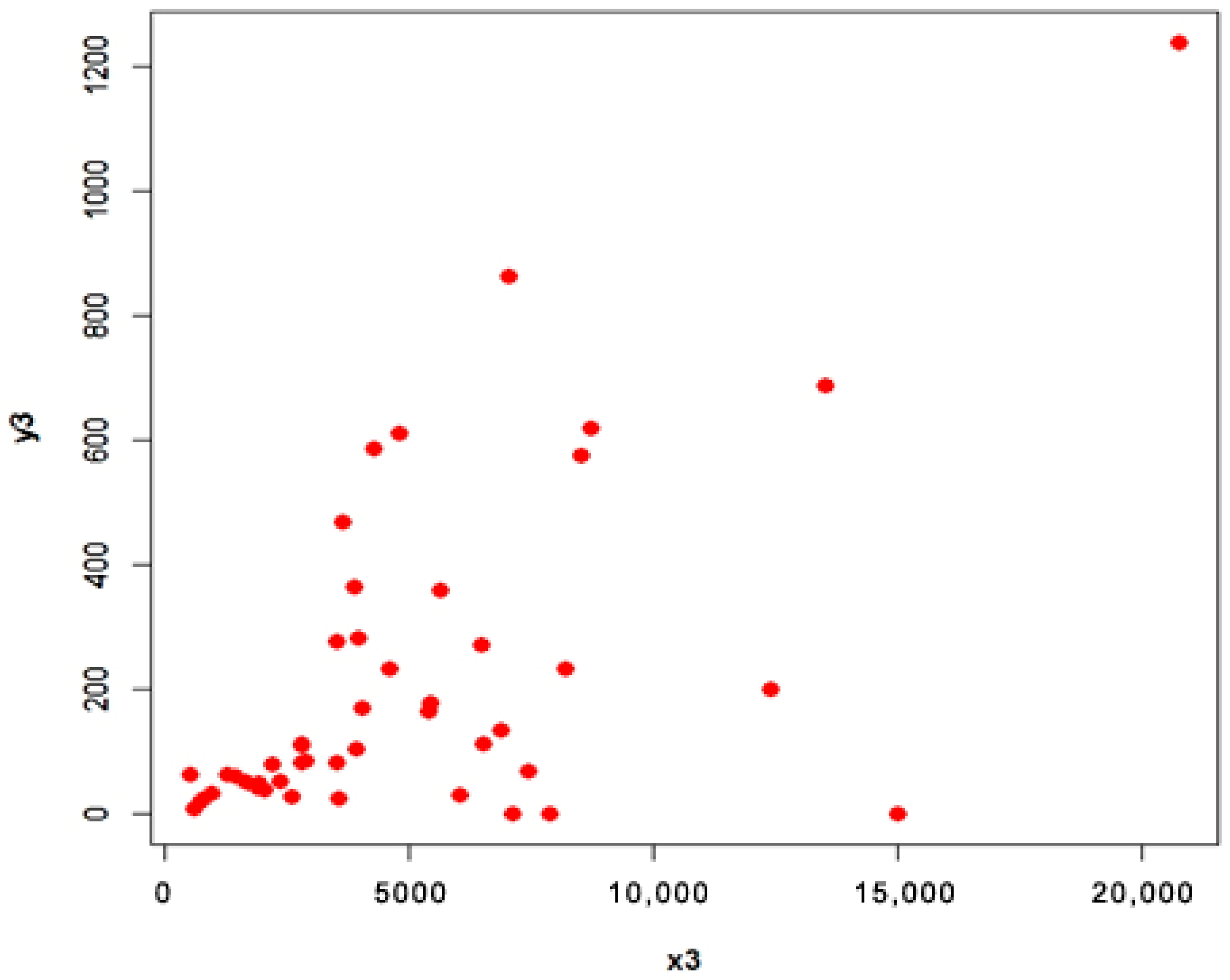
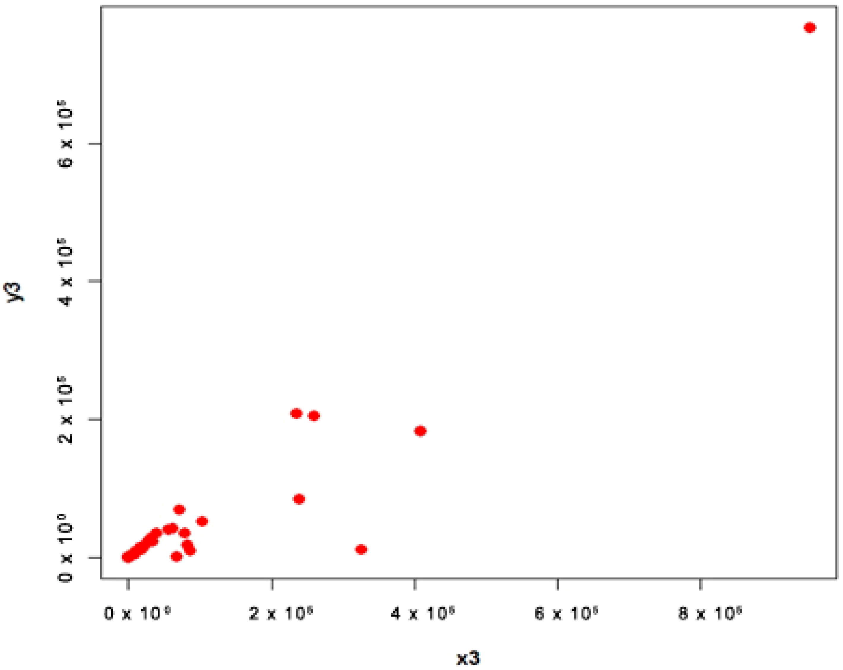
4.2. COVID-19 Data (Populations 3 and 4)
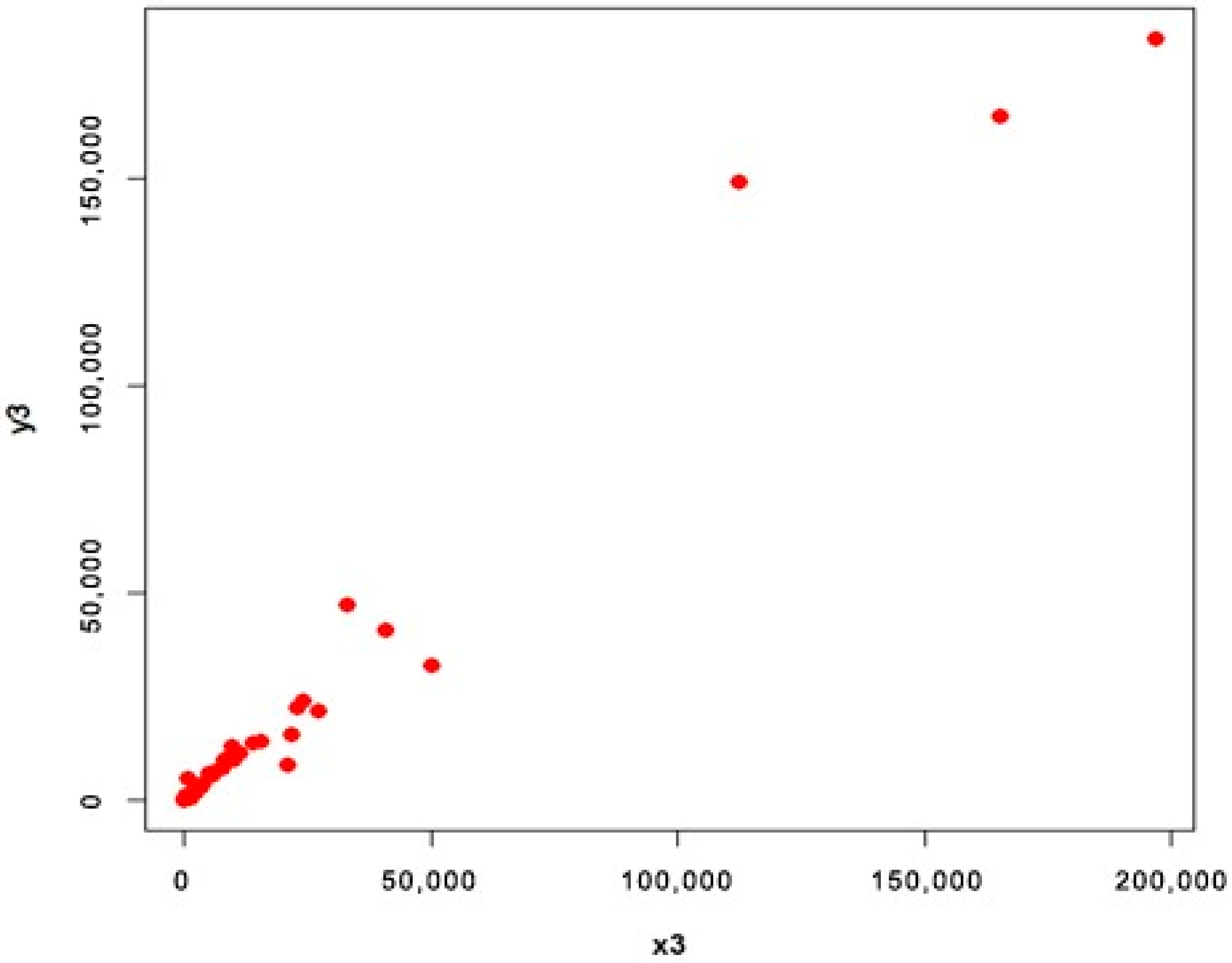
- Population 3
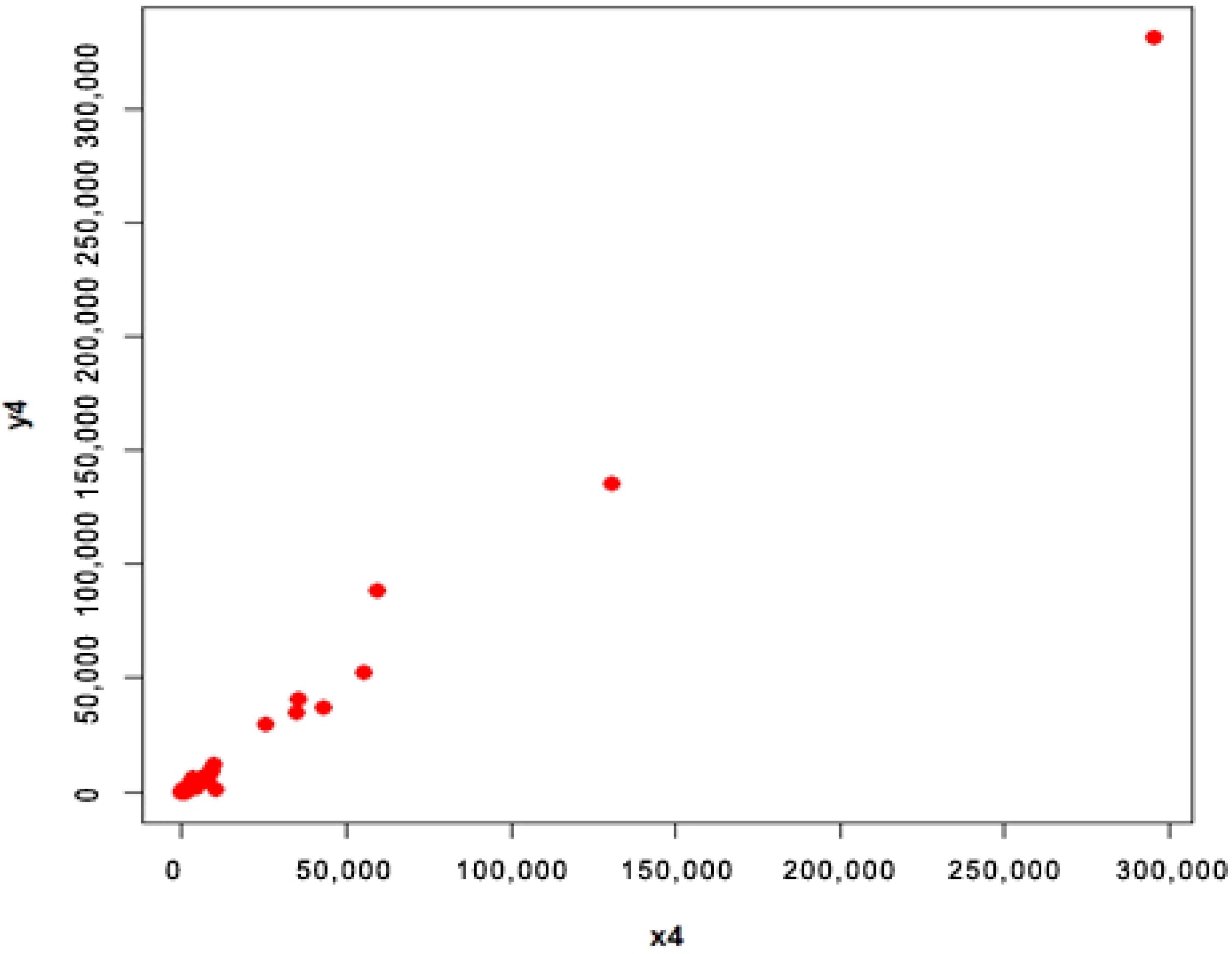
- Population 4
4.3. Interpretation
- For population 1, the first proposed estimator is better than first adapted estimator and the second proposed estimator is better than second adapted estimator at quantile ;
- For population 2, the first proposed estimator is better than first adapted estimator and the second proposed estimator is better than second adapted estimator at quantile ;
- For population 3, the first proposed estimator is better than first adapted estimator and the second proposed estimator is better than second adapted estimator at quantile ;
- For population 4, the first proposed estimator is better than first adapted estimator and the second proposed estimator is better than second adapted estimator at quantile .
5. Conclusions
Author Contributions
Funding
Institutional Review Board Statement
Informed Consent Statement
Data Availability Statement
Acknowledgments
Conflicts of Interest
References
- Chambers, R.L.; Dunstan, R. Estimating distribution functions from survey data. Biometrika 1986, 73, 597–604. [Google Scholar] [CrossRef]
- Rao, J.N.K.; Kovar, J.G.; Mental, H.J. On estimating distribution functions and quantiles from survey data using auxiliary information. Biometrika 1990, 77, 365–375. [Google Scholar] [CrossRef]
- Kuk, A.Y. A kernel method for estimating finite population distribution functions using auxiliary information. Biometrika 1993, 80, 385–392. [Google Scholar] [CrossRef]
- Chen, J.; Wu, C. Estimation of distribution function and quantiles using the model-calibrated pseudo empirical likelihood method. Stat. Sin. 2002, 12, 1223–1239. [Google Scholar]
- Singh, H.P.; Singh, S.; Kozak, M. A family of estimators of finite-population distribution function using auxiliary information. Acta Appl. Math. 2008, 104, 115–130. [Google Scholar] [CrossRef]
- Yaqub, M.; Shabbir, J. Estimation of population distribution function in the presence of non-response. Hacet. J. Math. Stat. 2018, 47, 471–511. [Google Scholar] [CrossRef]
- Akhlaq, T.; Ismail, M.; Shahbaz, M.Q. On Efficient Estimation of Process Variability. Symmetry 2019, 11, 554. [Google Scholar] [CrossRef]
- Hussain, S.; Ahmad, S.; Akhtar, S.; Javed, A.; Yasmeen, U. Estimation of finite population distribution function with dual use of auxiliary information under non-response. PLoS ONE 2020, 15, e0243584. [Google Scholar] [CrossRef] [PubMed]
- Ahmad, S.; Hussain, S.; Zahid, E.; Iftikhar, A.; Hussain, S.; Shabbir, J.; Aamir, M. A Simulation Study: Population Distribution Function Estimation Using Dual Auxiliary Information under Stratified Sampling Scheme. Math. Probl. Eng. 2022, 2022, 3263022. [Google Scholar] [CrossRef]
- Ahmad, S.; Aamir, M.; Hussain, S.; Shabbir, J.; Zahid, E.; Subkrajang, K.; Jirawattanapanit, A. A new generalized class of exponential factor-type estimators for population distribution function using two auxiliary variables. Math. Probl. Eng. 2022, 2022, 2545517. [Google Scholar] [CrossRef]
- Deville, J.C.; Särndal, C.E. Calibration estimators in survey sampling. J. Am. Stat. Assoc. 1992, 87, 376–382. [Google Scholar] [CrossRef]
- Tracy, D.S.; Singh, S.; Arnab, R. Note on calibration in stratified and double sampling. Surv. Methodol. 2003, 29, 99–104. [Google Scholar]
- Koyuncu, N.; Kadilar, C. Calibration Weighting in Stratified Random Sampling. Commun. Stat. Simul. Comput. 2016, 45, 2267–2275. [Google Scholar] [CrossRef]
- Ozgul, N. New Calibration Estimator Based on Two Auxiliary Variables in Stratified Sampling. Commun. Stat.—Theory Methods 2019, 48, 1481–1492. [Google Scholar] [CrossRef]
- Lata, A.S.; Rao, D.; Khan, M.G. Calibration estimation using proposed distance function. In Proceedings of the 2017 4th Asia-Pacific World Congress on Computer Science and Engineering (APWC on CSE), Mana Island, Fiji, 11–13 December 2017; pp. 162–166. [Google Scholar]
- Shahzad, U.; Ahmad, I.; Almanjahie, I.; Al-Noor, N.H.; Hanif, M. A new class of L-Moments based calibration variance Estimators. Comput. Mater. Contin. 2021, 66, 3013–3028. [Google Scholar] [CrossRef]
- Shahzad, U.; Ahmad, I.; Almanjahie, I.; Hanif, M.; Al-Noor, N.H. L-Moments and calibration based variance estimators under double stratified random sampling scheme: An application of covid-19 pandemic. Sci. Iran. 2023, 30, 814–821. [Google Scholar] [CrossRef]
- Naz, F.; Nawaz, T.; Pang, T.; Abid, M. Use of nonconventional dispersion measures to improve the efficiency of ratio-type estimators of variance in the presence of outliers. Symmetry 2019, 12, 16. [Google Scholar] [CrossRef]
- Zaman, T.; Bulut, H. Robust calibration for estimating the population mean using stratified random sampling. Sci. Iran. 2023, in press. [CrossRef]
- Shahzad, U.; Ahmad, I.; Almanjahie, I.; Al-Noor, N.H. L-Moments based calibrated variance estimators using double stratified sampling. Comput. Mater. Contin. 2021, 68, 3411–3430. [Google Scholar] [CrossRef]
- Shahzad, U.; Ahmad, I.; Garcia Luengo, A.V.; Zaman, T.; Al-Noor, N.H.; Kumar, A. Estimation of coefficient of variation using calibrated estimators in double stratified random sampling. Mathematics 2023, 11, 252. [Google Scholar] [CrossRef]


| Estimator | ||||
|---|---|---|---|---|
| Population 1 | 2.020741 | 1.240396 | 1.51145 | 0.9898991 |
| Population 2 | 2.525566 | 1.871007 | 2.026478 | 1.421637 |
| Population 3 | 0.8161305 | 0.8058786 | 0.7483107 | 0.7522832 |
| Population 4 | 8.117104 | 9.373521 | 6.609163 | 5.893258 |
| Estimator | ||||
|---|---|---|---|---|
| Population 1 | 4.083395 | 1.538583 | 2.284482 | 0.9799003 |
| Population 2 | 6.378484 | 3.500668 | 4.106615 | 2.021053 |
| Population 3 | 0.666069 | 0.6494403 | 0.5599689 | 0.56593 |
| Population 4 | 65.88738 | 87.86289 | 43.68103 | 34.73049 |
| Population 1 | Population 2 | Population 3 | Population 4 |
|---|---|---|---|
Disclaimer/Publisher’s Note: The statements, opinions and data contained in all publications are solely those of the individual author(s) and contributor(s) and not of MDPI and/or the editor(s). MDPI and/or the editor(s) disclaim responsibility for any injury to people or property resulting from any ideas, methods, instructions or products referred to in the content. |
© 2023 by the authors. Licensee MDPI, Basel, Switzerland. This article is an open access article distributed under the terms and conditions of the Creative Commons Attribution (CC BY) license (https://creativecommons.org/licenses/by/4.0/).
Share and Cite
Abbasi, H.; Hanif, M.; Shahzad, U.; Emam, W.; Tashkandy, Y.; Iftikhar, S.; Shahzadi, S. Calibration Estimation of Cumulative Distribution Function Using Robust Measures. Symmetry 2023, 15, 1157. https://doi.org/10.3390/sym15061157
Abbasi H, Hanif M, Shahzad U, Emam W, Tashkandy Y, Iftikhar S, Shahzadi S. Calibration Estimation of Cumulative Distribution Function Using Robust Measures. Symmetry. 2023; 15(6):1157. https://doi.org/10.3390/sym15061157
Chicago/Turabian StyleAbbasi, Hareem, Muhammad Hanif, Usman Shahzad, Walid Emam, Yusra Tashkandy, Soofia Iftikhar, and Shabnam Shahzadi. 2023. "Calibration Estimation of Cumulative Distribution Function Using Robust Measures" Symmetry 15, no. 6: 1157. https://doi.org/10.3390/sym15061157
APA StyleAbbasi, H., Hanif, M., Shahzad, U., Emam, W., Tashkandy, Y., Iftikhar, S., & Shahzadi, S. (2023). Calibration Estimation of Cumulative Distribution Function Using Robust Measures. Symmetry, 15(6), 1157. https://doi.org/10.3390/sym15061157