An Asymmetric Collision-Free Optimal Trajectory Planning Method for Three DOF Industrial Robotic Arms

Abstract

To improve the speed and dynamic adaptability of robotic arm trajectory planning, a collision-free optimal trajectory planning method combining non-uniform adaptive time meshing and bounding box collision detection was proposed. First, the dynamics and objective function of the asymmetric industrial robotic arm with three degrees of freedom (DOF) was formulated in the form of the dynamic optimization problem. Second, the control vector parameterization (CVP) was improved to enhance the computational performance of the problem. The discrete grid was adaptively adjusted according the trend of control variables. Then, a quick and effective collision detection strategy was used to avoid obstacles and to speed up calculation efficiency. The non-collision constraint is built by transforming the collision detection into the distance between two points, and then is combined into the dynamic optimization problem. The solution of the new optimization problem with the improved CVP leads to the higher calculation performance and the avoidance of obstacles. Lastly, the Siemens Manutec R3 robotic arm is taken as an example to verify the effectiveness of the planning method. The approach not only reduces computation time but also maintains accurate calculations, so that optimal trajectory can be selected from symmetric paths near the obstacles. When weights were set as λ₁ = λ₂ = 0.5, the solution efficiency was improved by 33%, and the minimum distance between the robotic arm and obstacle could be 0.08 m, which ensured that there was no collision.

1. Introduction

In recent years, industrial robotic arms (RA) have been widely used in various industrial production fields, such as welding, assembly, grinding, cutting, palletizing and spraying, due to their flexibility, high efficiency, high precision, repeatability, etc. As a result of the constant increase in the complexity of the production environment and the requirements of production efficiency, solving the optimal trajectory problem (OTP) efficiently has evolved into a crucial task in the use of the robotic arm [1].

OTP is essentially a nonlinear optimal control problem (OCP) with complex constraints. In general, by optimizing the control vector, the RA reaches a predetermined terminal state from an initial state under a series of complex constraints [2]. At present, the solution method for OCP includes numerical methods and heuristic algorithms, etc. [3]. Typical representatives of numerical methods are orthogonal collocation and CVP. The nonlinear programming (NLP) problem generated by OCP through CVP discretization has a smaller dimension and the results obtained are more accurate, so the CVP is widely used to solve OCP. However, solving NLP problems requires multiple processing of differential equations. In order to obtain more precise optimization results and increase the efficiency of the solution, it is necessary to optimize the time grid partition to make it more similar to the actual control curve of the decision variable with fewer time grids [4]. Therefore, researchers have proposed their time grid optimization strategies. Combined with grid partition, Liu et al. proposed a fast CVP algorithm based on the fourth-order Runge-Kutta. The approximation strategy improves the solution efficiency by increasing the ratio between the control variable parameters and the number of integral nodes in the solution of differential equations [5]. Shi et al. proposed a non-uniform CVP, in which the control vector and the length of each grid are solved as decision variables [6]. Guo et al. proposed a CVP based on orthogonal design, which builds a temporal grid based on the range obtained from orthogonal experiments [7]. The experimental study showed that the above-improved methods can greatly cut down on solving time while maintaining the solution’s accuracy.

Moreover, the RA will undoubtedly run into obstacles while moving due to the intricacy of the working environment. Consequently, when planning the manipulator’s trajectory, obstacle avoidance must be taken into full account. Collision-free trajectory planning, which is being investigated by numerous researchers, depends on an accurate collision detection algorithm. The bounding box collision detection (BBCD) was developed to effectively obtain the ideal trajectory, streamline object-to-object collision detection, and decrease detection complexity [8]. Zhao et al. obtained the optimal trajectory by combining the oriented bounding box (OBB) with the ant colony algorithm [9]. Hou designed the hierarchical axis-aligned bounding box (AABB), which can effectively implement the obstacle avoidance function of the manipulator [10]. Yang made an improvement to the storage method of the AABB in the planning process, improving the computational efficiency of optimal trajectories [11]. Fu combined the cylinder bounding box (CBB) with the artificial potential field and also planned collision-free optimal trajectories [12]. Wang used the OBB to obtain smooth RA trajectories [13]. Gan proposed an improved hybrid bounding box and changed the detection traversal rules to improve the computational efficiency while meeting the accuracy requirements [14]. Based on the idea of a sphere bounding box (SBB) and spatial superposition, Zhu simplifies the description of the spatial relationship between the obstacle and the manipulator to check whether there is a collision [15].

The solution strategy directly affects the efficiency and accuracy of the solution. If we require high precision but the calculation is heavy and the calculation time is long, it is difficult to perform real-time trajectory planning. On the contrary, the robot arm is likely to collide with obstacles or the RA cannot reach the target point. For BBCD, if the bounding box is not selected properly, it usually generates a large amount of redundant space in the box, which is not good for trajectory planning. To improve the rapidness and dynamic adaptability of RA trajectory planning, an optimal trajectory calculation method that combines BBCD and non-uniform adaptive time meshing is proposed in this paper.

The rest of this paper is organized as follows. Section 2 depicts the dynamics model of the Siemens Manutec R3 3-DOF asymmetric industrial robotic arm (R3-RA, The Siemens Inc., Munich, Germany) and the optimal trajectory problem. Section 3 presents the grid adaptive CVP (GA-CVP) method and performs simulation comparison under MATLAB 2020b (The MathWorks Inc., Natick, MA, USA). Section 4 presents the multi-sphere BBCD method and performs simulation comparison under MATLAB 2020b. Section 5 summarizes the work of this paper.

2. Problem Description

Figure 1 shows the R3-RA, which is used for simulation in this study. It has three rotational axis, positive for counterclockwise rotation. $q_i$ describes the relative angle between arm $i-1$ and arm i for $i=1,2,3$. In the following article, $\theta$ is used to represent q.

The asymmetric dynamics model of R3-RA is shown below [16,17,18]:

$$\begin{array}{c}\hfill \mathit{M}\left(\mathit{\theta }\left(t\right)\right)·\ddot{\mathit{\theta }}\left(t\right)=\mathit{D}\mathit{·}\mathit{u}\left(t\right)+C(\dot{\mathit{\theta }}\left(t\right),\mathit{\theta }\left(t\right))+\mathit{G}\left(\mathit{\theta }\left(t\right)\right)\end{array}$$

(1)

Hereby, $\mathit{\theta }\left(t\right)={[{\theta }_1\left(t\right),{\theta }_2\left(t\right),{\theta }_3\left(t\right)]}^T$ is the rotation angle between adjacent links on the joint axis, in $\mathrm{rad}$; $\dot{\mathit{\theta }}\left(t\right)$ is the relative angular velocity on the joint axis, in $\mathrm{rad}/\mathrm{s}$; $\ddot{\mathit{\theta }}\left(t\right)$ is the relative plus angular velocity on the joint axis, in $\mathrm{rad}/{\mathrm{s}}^2$; $\mathit{u}\left(t\right)={[u_1\left(t\right),u_2\left(t\right),u_3\left(t\right)]}^T$ is the time-dependent torque voltage on the joint axis, in $\mathrm{V}$; $\mathit{D}$ is $3\times 3$ diagonal constant matrix; $\mathit{M}\left(\mathit{\theta }\right)$ is $3\times 3$ positive-definite symmetric mass matrix containing rotational inertia. $\mathit{\theta }$ is a simplified form of $\mathit{\theta }\left(t\right)$, which is also a variable for time t. $\mathit{M}\left(\mathit{\theta }\right)$ is shown in Equation (2).

$$\begin{array}{c}{\mathit{M}}_{1,1}\left(\mathit{\theta }\right)=c_1{sin}^2\left({\theta }_2+{\theta }_3\right)+c_{2}sin\left({\theta }_2+{\theta }_3\right)sin\left({\theta }_2\right)\hfill \\ +c_3{sin}^2\left({\theta }_2\right)\hfill \\ {\mathit{M}}_{1,2}\left(\mathit{\theta }\right)=c_{7}cos\left({\theta }_2+{\theta }_3\right)+c_{8}cos\left({\theta }_2\right)\hfill \\ {\mathit{M}}_{1,3}\left(\mathit{\theta }\right)=c_{7}cos\left({\theta }_2+{\theta }_3\right)\hfill \\ {\mathit{M}}_{2,2}\left(\mathit{\theta }\right)=c_{2}cos\left({\theta }_3\right)+c_9\hfill \\ {\mathit{M}}_{2,3}\left(\mathit{\theta }\right)=c_{10}cos\left({\theta }_3\right)+c_{11}\hfill \\ {\mathit{M}}_{3,3}\left(\mathit{\theta }\right)=c_{12}\hfill \end{array}$$

(2)

Hereby, $c{}_i\left(i=1,2,\dots ,12\right)$ is constant, as

Table 1. R3-RA Parameters.

Parameter	Numerical Value	Parameter	Numerical Value
$c_1$	8.0604812 + 0.9601m	$c_8$	−3.2963900
$c_2$	12.1806 + 0.98m	$c_9$	85.2298937 + 1.2104m
$c_3$	20.1794125 + 0.25m	$c_{10}$	6.0903 + 0.49m
$c_4$	0.39	$c_{11}$	7.9484812 + 0.9604m
$c_5$	0.64	$c_{12}$	12.5504812 + 0.9604m
$c_6$	17.2112712	$b_1$	(12.1806 + 0.98m)g
$c_7$	−0.0110568	$b_2$	(41.7325 + 0.50m)g

shown.

$C(\dot{\mathit{\theta }},\mathit{\theta })$ is the torque caused by Coriolis and centrifugal forces and has the following structure for $i=1,2,3$:

$$\begin{array}{c}C(\dot{\mathit{\theta }},\mathit{\theta })={\displaystyle \sum _{j=1}^3}[{\displaystyle \sum _{k=1}^3}{\Gamma }_{i,j,k}\left(\mathit{\theta }\right){\dot{\theta }}_k]{\dot{\theta }}_j\hfill \\ {\Gamma }_{i,j,k}\left(\mathit{\theta }\right)=-\frac{1}{2}[\frac{\partial M_{ij}\left(\mathit{\theta }\right)}{\partial {\theta }_k}+\frac{\partial M_{i,k}\left(\mathit{\theta }\right)}{\partial {\theta }_j}-\frac{\partial M_{j,k}\left(\mathit{\theta }\right)}{\partial {\theta }_i}]\hfill \end{array}$$

(3)

$\mathit{G}\left(\theta \right)$ is the torque due to the gravitational force, as shown in the following equation.

$$\begin{array}{c}{\mathit{G}}_1^g\left(\mathit{\theta }\right)=0\hfill \\ {\mathit{G}}_2^g\left(\mathit{\theta }\right)=b_{1}cos\left({\theta }_2\right)sin\left({\theta }_3\right)+b_{1}sin\left({\theta }_2\right)cos\left({\theta }_3\right)+b_{2}sin\left({\theta }_2\right)\hfill \\ {\mathit{G}}_3^g\left(\mathit{\theta }\right)=b_{1}sin\left({\theta }_2+{\theta }_3\right)\hfill \end{array}$$

(4)

Hereby, $b_i(i=1,2)$ is a constant, as Table 1 shown. In Table 1, $m=15 \mathrm{k}\mathrm{g}$ is transport load, $g=9.81 \mathrm{m}/{\mathrm{s}}^2$ is gravity constant.

When the time optimal is the goal of trajectory planning, we can obtain the objective function [19]:

$$min{J}_1=t_f$$

(5)

where, $t_f$ is the time required for the manipulator to complete its trajectory, also known as the terminal time.

With energy optimisation as the goal of trajectory planning, we can obtain the objective function [20]:

$$\begin{array}{c}\hfill min{J}_2={\int }_0^{t_f}{\displaystyle \sum _{i=1}^n}{u}_i{\left(t\right)}^2\mathrm{d}t\end{array}$$

(6)

where, $u_i\left(t\right)$ is the torque voltage on the corresponding joint axis, $i=1,\dots ,n$. n is the number of robot joints.

According to Equations (5) and (6), when the integrated optimization of time and energy is the goal of trajectory planning, we obtain the objective function [21]:

$$\begin{array}{c}\hfill minJ={\lambda }_1{t}_f+{\lambda }_2{\int }_0^{t_f}{\displaystyle \sum _{i=1}^n}{u}_i{\left(t\right)}^2\mathrm{d}t\end{array}$$

(7)

where, ${\lambda }_1$ and ${\lambda }_2$ are the weighting factors for the energy and time terms. The two weights can be manually set, but ${\lambda }_1+{\lambda }_2=1$ must be satisfied. The remaining variables have the same meaning as Equations (5) and (6).

According to Equations (1)–(4), considering obstacle avoidance, the mathematical expression for the OTP of the R3-RA is as follows:

$$\begin{array}{c}\hfill \begin{array}{c}\underset{U_i\left(t\right)t_f}{min}J={\lambda }_1{t}_f+{\lambda }_2{\int }_0^{t_f}{\displaystyle \sum _{i=1}^n}{u}_i{\left(t\right)}^2\mathrm{d}t\hfill \\ \mathrm{s}.\mathrm{t} \dot{\mathit{v}}\left(t\right)=\mathit{M}{\left(\mathit{\theta }\left(t\right)\right)}^{-1}·[\mathit{D}·\mathit{u}\left(t\right)+C\left(\mathit{v}\left(t\right),\mathit{\theta }\left(t\right)\right)+\mathit{G}\left(\mathit{\theta }\left(t\right)\right)]\hfill \\ \mathit{\theta }\left(0\right)={\theta }_{\mathrm{initial}}\mathit{\theta }\left(t_f\right)={\mathit{\theta }}_{\mathrm{target}}\hfill \\ \mathit{v}\left(0\right)=\mathbf{0}\mathit{v}\left(t_f\right)=\mathbf{0}\hfill \\ \underline{\mathit{u}}\le \mathit{u}\left(t\right)\le \overline{\mathit{u}}\underline{\mathit{\theta }}\le \mathit{\theta }\left(t\right)\le \overline{\mathit{\theta }}\underline{\mathit{v}}\le \mathit{v}\left(t\right)\le \overline{\mathit{v}}t\in [0,t_f]\hfill \\ d_i\left(t\right)>0i=1,2,\dots ,n\hfill \end{array}\end{array}$$

(8)

where, $\mathit{v}\left(t\right)=\dot{\mathit{\theta }}\left(t\right)$. $d_i\left(t\right)$ is the distance of the ith joint of the robot arm to the obstacle at the t moment, and if the distance is greater than 0, the collision-free trajectory can be generated. RA starts at $t=0$ and ends at $t=t_f$. According to the theory of inverse kinematics, the initial joint angle ${\mathit{\theta }}_{\mathrm{initial}}$ and the target joint angle ${\mathit{\theta }}_{\mathrm{target}}$ can be calculated based on the known initial state and target state of RA’s position. Moreover, it has a constraint such that the angular velocity of each joint of the robot is 0 when the RA is in initial state and target state. The torque voltage on each joint axis, each joint angle and angular velocity are in line with its upper and lower limits. In this study, R3-RA has three joints, so $n=3$.

3. Control Vector Parameter Based on Grid Adaptation

CVP discretizes the control variables in the whole horizon by grid partition, divides them into components corresponding to time subintervals, and uses the polynomial approximation method with finite parameters to approximately represent the components so that we have finite-dimensional static NLP problems [22]. Therefore, we adopt a slope-based GA-CVP, which greatly reduces the computational burden after grid refinement.

3.1. Grid Reconfiguration Strategy

The uniform discretization-based control vector parameterization is unified and fixed. To approximate the control variable well, the whole control horizon must be partitioned very densely [23]. However, too many time grids will lead to a sharp increase in computation.

Figure 2 shows that the slope can well reflect the variation of the control variable throughout the control time domain. The control variables in the time interval $\left[t_{0,}{t}_a\right]$ are exponentially decreasing with a sharp change in slope. The control variables in the time interval $[t_a,t_b]$ are flatter with a smaller change in slope. The change in the slope of the control variable between each adjacent time subinterval reflects the above phenomenon well. The increasing slope will cause the curve of the control variable will change significantly, so it is necessary to refine the time subinterval $[t_0,t_a]$ and increase the number of time grids, so as to improve its approximation accuracy. When the slope gradually decreases, it means that the control variables change little or hardly at all. Thus, it does not require too many time grids. By doing this, the number of time grids in the time subinterval $[t_a,t_b]$ can be reduced in the time subinterval $[t_a,t_b]$ and eliminating the redundant grids, thus reducing the dimensionality of NLP and also the time required for the computation.

As shown in Figure 3, the following two slope information is defined within the left and right time subintervals $[t_{j,i-1},t_{j,i}]$ and $[t_{j,i},t_{j,i+1}]$ of the time node $t_{j,i}$.

The left slope of the time node $t_{j,i}$ $s_{j,i}^{-}$.

$$\begin{array}{c}\hfill s_{j,i}^{-}=\frac{C_{j,i+1}-C_{j,i}}{t_{j,i}-t_{j,i-1}}\end{array}$$

(9)

The right slope of the time node $t_{j,i}$ of $s_{j,i}^{+}$.

$$\begin{array}{c}\hfill s_{j,i}^{+}=\frac{C_{j,i+1}-C_{j,i}}{t_{j,i+1}-t_{j,i}}\end{array}$$

(10)

where, $C_{j,i}$, $C_{j,i+1}$ are the time subintervals $[t_{j,i-1},t_{j,i}]$ and $[t_{j,i},t_{j,i+1}]$ of the control parameters.

3.1.1. Merging of Time Grid Nodes

The purpose of merging time grid nodes is to eliminate the time subintervals that have less impact on the accuracy of the approximation in the parameterization process, and to reduce the number of unnecessary parameters. Thus, it can reduce the dimensionality of the nonlinear programming and shorten the time for the calculation. Equation (11) shows the rules for merging time grid.

$$\begin{array}{c}\hfill \left|s_{j,i}^{-}\right|+\left|s_{j,i}^{+}\right|\le {\xi }_c\end{array}$$

(11)

where, ${\xi }_c$ is the merging factor.

If the left slope $t_{j,i}$ of the time node $s_{j,i}^{-}$ and the right slope $s_{j,i}^{+}$ satisfy the Equation (11), it means that this time node has little influence on the accuracy of the approximation, and the time node $t_{j,i}$ can be deleted, i.e., the time subinterval $[t_{j,i-1},t_{j,i}]$ and $[t_{j,i},t_{j,i+1}]$ can be merged. For the obtained subinterval $[t_{j,i-1},t_{j,i+1}]$ after merging, the values of its control parameters are the average of the control parameters $C_{j,i}$ and $C_{j,i+1}$.

3.1.2. Insertion of Time Grid Nodes

When the control variable curve changes rapidly and the slope is large enough, the time subinterval corresponding to this part of the curve needs to be divided using more grids to improve the approximation accuracy for the control variable curve. Equations (12) and (13) show the rules for inserting the time grid nodes.

$$\begin{array}{c}\hfill \Delta k_1=\left\{\begin{array}{cc}1& \left(\left|s_{j,i}^{-}\right|\right)\in \left[{\xi }_1,{\xi }_2\right)\\ 2& \left(\left|s_{j,i}^{-}\right|\right)\in \left[{\xi }_2,{\xi }_3\right)\\ ⋮& ⋮\\ m_{\xi }-1& \left(\left|s_{j,i}^{-}\right|\right)\in \left[{\xi }_{m_{\xi }-1},{\xi }_{m_{\xi }}\right)\end{array}\right.\left|s_{j,i}^{-}\right|\ne 0\end{array}$$

(12)

$$\begin{array}{c}\hfill \Delta k_2=\left\{\begin{array}{cc}1& \left(\left|s_{j,i}^{+}\right|\right)\in \left[{\xi }_1,{\xi }_2\right)\\ 2& \left(\left|s_{j,i}^{+}\right|\right)\in \left[{\xi }_2,{\xi }_3\right)\\ ⋮& ⋮\\ m_{\xi }-1& \left(\left|s_{j,i}^{+}\right|\right)\in \left[{\xi }_{m_{\xi }-1},{\xi }_{m_{\xi }}\right)\end{array}\right.\left|s_{j,i}^{+}\right|\ne 0\end{array}$$

(13)

where, ${\xi }_i(i=1,2,\dots ,m_{\xi })$ is the insertion coefficient, $\Delta k_1$ and $\Delta k_2$ are both the number of insertion time nodes.

For the time nodes $t_{j,i}$ with left and right slopes $s_{j,i}^{-}$ and $s_{j,i}^{+}$, if Equations (12) and (13) are satisfied, $[t_{j,i-1},t_{j,i}]$ and $[t_{j,i},t_{j,i+1}]$ are inserted with the corresponding number of time nodes. Through merging and inserting grid node, the grid becomes non-uniform and asymmetric, avoiding unnecessary computations.

3.1.3. Algorithm Termination Conditions

By reconstructing the temporal grid, the next iteration of the optimized post-temporal grid division can be obtained. So on and so forth, until the termination condition is satisfied. GA-CVP solution algorithm termination conditions are mainly the following two kinds.

The first one is set to the number of iterations L, which is greater than the upper limit $L_{max}$.

$$\begin{array}{c}\hfill L>L_{max}\end{array}$$

(14)

The second one is that the difference between the absolute values of the two objective function values $J^{L+1}$ and $J^L$ obtained from the $L+1$th and Lth iterations is less than the allowable error.

$$\begin{array}{c}\hfill \left|\left|J^{L+1}\right|-\left|J^L\right|\right|<{\xi }_J\end{array}$$

(15)

where, ${\xi }_J$ is the allowable error of the difference between the absolute values of the objective function values $J^{L+1}$ and $J^L$.

3.2. Algorithm Steps and Flow Chart

Figure 4 shows the flow chart of GA-CVP.

Step 1: set the iteration number $L=0$, the initial number of discrete-time lattices $N^{\left(0\right)}$ and the initial values of the control parameters ${C_{j,i}}^{\left(0\right)}$ for each time lattice, the merging coefficients ${\xi }_c$, the insertion coefficients ${\xi }_i(i=1,2,\dots ,m_{\xi })$, the tolerance error ${xi}_J$ and the upper limit of iterations $L_{max}$.

Step 2: based on the discretized control parameters, ${C_{j,i}}^{\left(L\right)}$ solves the initial value problem of the differential equation consisting of $N^{\left(L\right)}$ time grids discretized to obtain the state variables and the objective function value of this cycle $\tilde{J}\left({C_{j,i}}^{\left(L\right)}\right)$ under the current discrete grid number.

Step 3: determine whether the termination condition is satisfied, and if so, jump out of the loop and return the current optimal value. Otherwise, according to the control parameters ${C_{j,i}}^{\left(L\right)}$ and the number of time grids $N^{\left(L\right)}$, calculate the left and right slopes of each time node under the current number of time grids. Based on the merged time node rule Equation (11) and the inserted time node rule Equations (12) and (13), calculate the refined time grid number $N^{(L+1)}$ and its corresponding control parameters ${C_{j,i}}^{(L+1)}$. Let $L=L+1$ and proceed to step 2.

3.3. Numerical Results

Equation (16) is the initial state, target state and constraints of OTP(8) without obstacles.

$$\begin{array}{c}\hfill \begin{array}{c}\mathit{\theta }\left(0\right)=[0 \mathrm{rad},-1.5 \mathrm{rad},0 \mathrm{rad}]\mathit{\theta }\left(t_f\right)=[1 \mathrm{rad},-1.95 \mathrm{rad},1 \mathrm{rad}]\hfill \\ v_i\left(0\right)=0 \mathrm{rad}/\mathrm{s}{v}_i\left(t_f\right)=0 \mathrm{rad}/\mathrm{s}\left|{\mathit{u}}_i\left(t\right)\right|\le 7.5 \mathrm{V}i=1,2,3\hfill \\ \left|{\theta }_1\left(t\right)\right|\le 2.97 \mathrm{rad}\left|{\theta }_2\left(t\right)\right|\le 2.01 \mathrm{rad}\left|{\theta }_3\left(t\right)\right|\le 2.86 \mathrm{rad}\hfill \\ \left|v_1\left(t\right)\right|\le 3.0 \mathrm{rad}/\mathrm{s}\left|v_2\left(t\right)\right|\le 1.5 \mathrm{rad}/\mathrm{s}\left|v_3\left(t\right)\right|\le 5.2 \mathrm{rad}/\mathrm{s}t\in [0,t_f]\hfill \end{array}\end{array}$$

(16)

The three initial control parameters are set to the mean values of the respective control variables $u_i\left(t\right) (i=1,2,3)$ constrained. The weighting coefficients are set as ${\lambda }_1={\lambda }_2=0.5$. The joint space under the task requirement can be obtained by MATLAB simulation calculation. Figure 5 shows the angle variation of each joint. Figure 6 shows the corresponding angular velocity variation of each joint.

From Figure 5, it can be obtained that the trajectories by UD-CVP and GA-CVP, the the joint angle variables at the initial moment and the joint angle variables at the terminal moment meet the task requirements, indicating that the end of the R3 can move accurately from the initial position to the target position. Moreover, each joint angle during the motion is within the range of the constraints. Each angle changing of each joint is smooth, but the angle changing of each joint obtained by GA-CVP is smoother. From Figure 6, it can be seen that the trajectories obtained by UD-CVP and GA-CVP, the joint angular velocity at the initial moment and the joint angular velocity at the terminal moment meet the task requirements. The angular velocity of each joint during the motion is within the range of the angular velocity constraints.

Table 2. Results of the OTP with integrated time and energy optimization (${\lambda }_1=0.99$, ${\lambda }_2=0.01$).

Method	Number of Iterations	Number of Parameters	Value	Calculation Time (s)	Sum of Time (s)
UD-CVP ($N=15$)	1	45	0.9933	17.2150	17.2150
UD-CVP ($N=50$)	1	150	0.9924	111.1380	111.1380
GA-CVP ($N=15$)	1	45	0.9933	17.2150	95.9480
	2	146	0.9924	78.7330

,

Table 3. Results of the OTP with integrated time and energy optimization (${\lambda }_1={\lambda }_2=0.5$).

Method	Number of Iterations	Number of Parameters	Value	Calculation Time (s)	Sum of Time (s)
UD-CVP ($N=15$)	1	45	13.2508	11.2360	11.2360
UD-CVP ($N=50$)	1	150	13.2279	108.8620	108.8620
GA-CVP ($N=15$)	1	45	13.2508	11.2360	39.9380
	2	141	13.2347	28.7020

and

Table 4. Results of OTP with integrated time and energy optimization (${\lambda }_1=0.01$, ${\lambda }_2=0.99$).

Method	Number of Iterations	Number of Parameters	Value	Calculation Time (s)	Sum of Time (s)
UD-CVP ($N=15$)	1	45	25.2566	15.3770	15.3770
UD-CVP ($N=50$)	1	150	25.2113	248.0260	248.0260
GA-CVP ($N=15$)	1	45	25.2566	15.3770	54.7670
	2	140	25.2248	39.3900

show the results of the OTP with three different weights. Comparing the results of UD-CVP with $N=15$ and $N=50$ for three different weights, it reveals that as the number of discrete-time grids N increases, the number of optimization parameters increases and the accuracy is improved, but the time for the solution also increases significantly. When ${\lambda }_1=0.99$ and ${\lambda }_2=0.01$, the objective function values obtained by the UD-CVP ($N=50$) and the GA-CVP ($N=15$) are the same, and the solution time required by the GA-CVP ($N=15$) is 86% of the UD-CVP ($N=50$). The solution efficiency is improved by 14%. Comparing Table 3 and Table 4 under two different weights, although the accuracy of the solution of the UD-CVP ($N=50$) is higher than that of the GA-CVP ($N=15$). The solution time required by the GA-CVP is shorter. When the weights take ${\lambda }_1=0.5$, ${\lambda }_2=0.5$, the solution time required by the GA-CVP is only 37% of the UD-CVP, and the solution efficiency is improved by 63% in this case. When the weights are taken as ${\lambda }_1=0.01$, ${\lambda }_2=0.99$, the solution time required by the GA-CVP is only 1/5 of the UD-CVP. The solution efficiency is improved by 78% in this case. The simulation demonstrates that the mesh redistribution based on the difference of slope is effective in improving the computational efficiency and shortening the solution time.

Table 5. Results of OTP with integrated time and energy optimization with different weights.

${\mathit{\lambda }}_1$	${\mathit{\lambda }}_2$	Value	${\mathit{J}}_1={\mathit{t}}_{\mathit{f}}$	${\mathit{J}}_2={\int }_0^{{\mathit{t}}_{\mathit{f}}}{\displaystyle \sum _{\mathit{i}=1}^{\mathit{n}}}{\mathit{u}}_{\mathit{i}}{\left(\mathit{t}\right)}^2\mathit{d}\mathit{t}$
0.99	0.01	0.9924	0.6406	35.81293814
0.9	0.1	3.4147	0.9127	25.93269761
0.75	0.25	7.1128	0.9884	25.48609053
0.5	0.5	13.2279	1	25.45583174
0.25	0.75	19.3419	1	25.45585704
0.01	0.99	25.2113	1	25.45582902

shows the results of the OTP with different optimization weights. When ${\lambda }_1$ is larger, the optimized center of gravity is biased towards time, so the time for the R3 to move from the initial position to the target position is relatively shorter, while its energy consumption is relatively larger. When ${\lambda }_2$ is larger, the center of gravity of optimization is biased towards energy. R3 consumes relatively less energy and takes relatively longer time to move from the initial position to the target position. When ${\lambda }_1\in [0,0.5)$, the optimized values of $J_1=t_f$ and $J_2={\int }_0^{t_f}{\displaystyle \sum _{i=1}^n}{u}_i{\left(t\right)}^2\mathrm{d}t$ change very little, so it is recommended that ${\lambda }_1$ is taken in the range of $[0.5,1]$.

4. Optimal Trajectory Planning for Robotic Arm with Obstacles

Whether the RA can successfully avoid obstacles, the key is to determine the distance $d_i\left(t\right)$ from the RA to the obstacles. Moreover, near the obstacle, it is easy to generate a symmetric path, and the RA needs to quickly optimize it to choose a better trajectory to move. If the modeling is based on the shape of the robot and the obstacle, for checking whether they collide at each moment, it will make the computational complexity much higher and the solution more difficult to obtain. Therefore, this study uses the bounding box detection method to simplify the collision detection object model and reduce the computational complexity.

4.1. Bounding Box Collision Detection

According to the shape characteristics of the bounding box, the bounding box can be classified as CBB, AABB, or SBB, etc. The computational complexity of collision detection decreases with the simplification of the bounding box shape. However, the simple shape may lead to poor envelope sealing to the envelope of the RA, which directly affects the collision detection sensitivity [24].

4.1.1. Collision Detection Based on Cylinder Bounding Box

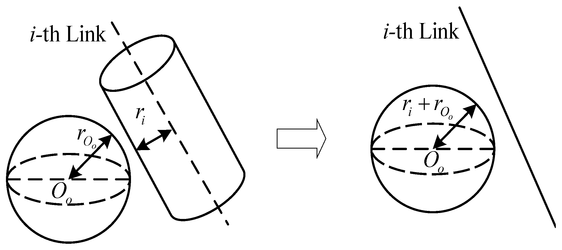
Figure 7 shows the spatial position relationship between the CBB of the i-th link of the RA and the obstacle. To simplify the calculation, the cylinder can be considered as a line segment, while the radius $r_i$ of the sphere surrounding the obstacle is increased by the radius $r_{O_o}$ of the cylinder. Thus, the collision detection problem is simplified into an intersection detection problem between a line and a ball in space.

The sphere of the obstacle has a centre of $O_o\left(x_{O_o},y_{O_o},z_{O_o}\right)$. The first and last coordinates of the i-th link of the robot are $(x_i,y_i,z_i)$, $(x_{i+1},y_{i+1},z_{i+1})$. From the centre $O_o$, a vertical line segment is drawn towards the link i and intersects the line segment at the point $P_i$. Suppose the coordinate of the foot point $P_i$ is $(x_{P_i},y_{P_i},z_{P_i})$. We obtain the equation of a straight line in space:

$$\begin{array}{c}\hfill \left\{\begin{array}{c}{x}_{P_i}={\alpha }_i\left(x_{i+1}-x_i\right)+x_i\hfill \\ y_{P_i}={\alpha }_i\left(y_{i+1}-y_i\right)+y_i\hfill \\ z_{P_i}={\alpha }_i\left(z_{i+1}-z_i\right)+z_i\hfill \end{array}\right.\end{array}$$

(17)

The coordinates of the foot point $P_i$ can be determined by the proportional coefficient ${\alpha }_i$ in the Equation (17). We will typically want to ensure that the robot has a safety margin $d_{\mathrm{safe}}$ [25]. Thus, we want to enforce the following constraints at each time step.

$$\begin{array}{c}\hfill \sqrt{{\left(x_{P_i}-x_{O_o}\right)}^2+{\left(y_{P_i}-y_{O_o}\right)}^2+{\left(z_{P_i}-z_{O_o}\right)}^2}-(r_{O_o}+r_k+d_{\mathrm{safe}})\ge 0i=1,2,\dots ,n\end{array}$$

(18)

4.1.2. Collision Detection Based on Multi-Sphere Bounding Box

The SBB uses a sphere with the smallest radius that can completely enclose the object to approximate the RA. The object is projected onto the coordinate axes, and the two points farthest apart are obtained. Take the midpoint of the line segment connecting the two points as the center of the sphere. The length of the line segment is used as the diameter of the sphere to construct the minimum SBB.

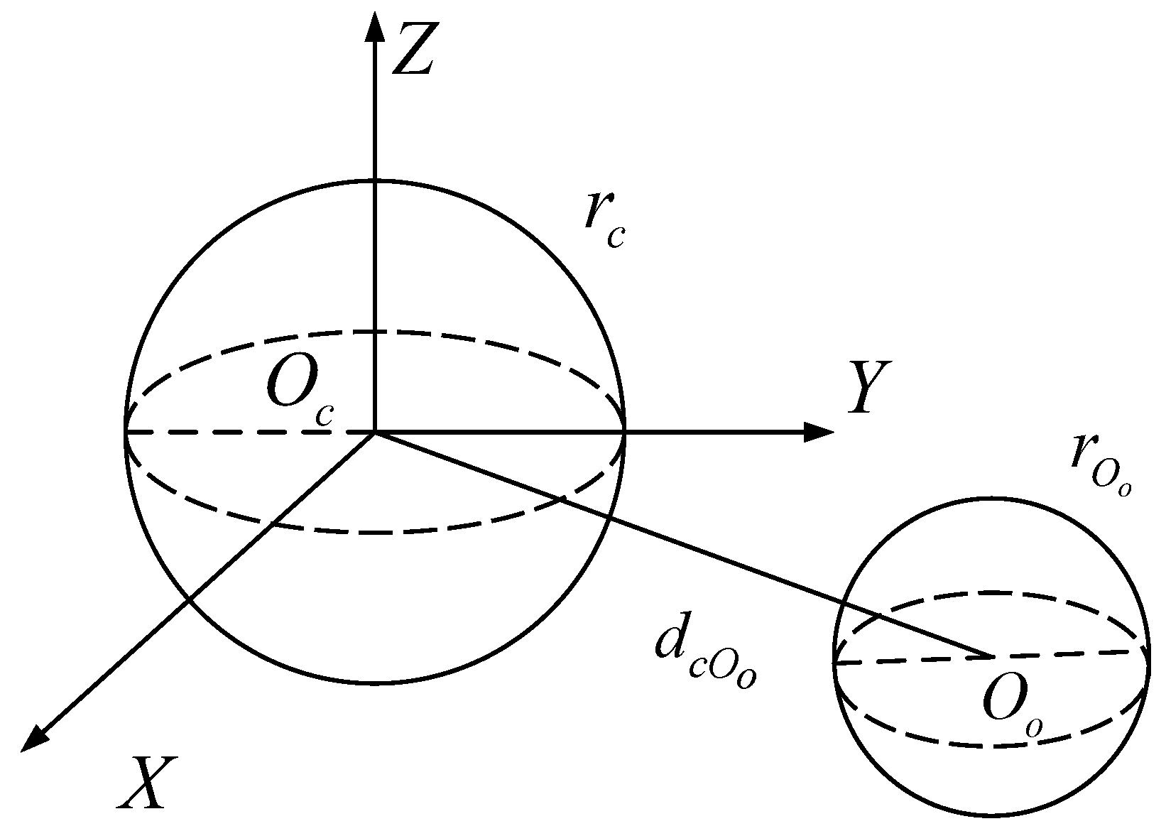
Suppose the coordinates of the center of the sphere are $O_c\left(x_c,y_c,z_c\right)$, and the radius of the sphere is $r_c$. The obstacle enveloped by a SBB, its spherical center and radius are $O_o\left(x_{O_o},y_{O_o},z_{O_o}\right)$ and $r_{O_o}$.

According Figure 8, the distance $d_{cd}$ between the centers of the two spheres can be calculated by the spatial expression of the two spheres.

$$\begin{array}{c}\hfill d_{c{O}_o}=∥O_c{O}_o∥=\sqrt{{\left(x_c-x_{O_o}\right)}^2+{\left(y_c-y_{O_o}\right)}^2+{\left(z_c-z_{O_o}\right)}^2}\end{array}$$

(19)

It is simple to check for collisions between R3-RA and obstacles by SBB. However, the distribution of the R3-RA over the three coordinate axes is not uniform. When R3-RA is enveloped by the SBB, there will be a large amount of redundant space inside, which will lead to a decrease in the accuracy of collision detection and a considerable increase in the solution time. After analyzing the shape of the R3-RA, we decided to use multiple spheres of different sizes to envelope the RA, so that it could compensate for the poor compactness.

Select a set of points $O_{i_k}$ on the centre line of the i-th link as the centre of the bounding sphere, and define the corresponding radius $r_{i_k}$. Make point $O_{k_i}$ as centre, such that the set $O_{i_k}=\left\{O_{i_k}\right|k=1,2,\dots ,N_{\mathrm{s}}\}$ of spheres can fully envelop the i-th link. Figure 9 shows the multi-sphere surrounding the RA.

Similarly, we want to enforce the following constraints at each time step.

$$\begin{array}{c}\hfill ∥O_{i_k}{O}_o∥-(r_{O_o}+r_k+d_{\mathrm{safe}})\ge 0i=1,2,\dots ,n\end{array}$$

(20)

Hereby, $O_{i_k}$ is the center of the k-th bounding ball on the i-th link, $k=1,2,\dots ,N_{\mathrm{s}}$, $N_{\mathrm{s}}$ is the number of bounding balls on the link. $∥O_{i_k}{O}_o∥$ can be specifically expressed by Equation (19).

4.2. Numerical Results

In order to more fully test the collision-free trajectory planning based on the two bounding box, we test them under two different task requirements. Task 1: ${\mathit{\theta }}_{\mathrm{initial}}=[0\mathrm{rad},-1.5\mathrm{rad},0\mathrm{rad}]$, ${\mathit{\theta }}_{\mathrm{target}}=[1\mathrm{rad},-1.95\mathrm{rad},1\mathrm{rad}]$. The coordinates of the ball centre surrounding the obstacles are $\left(0.26 \mathrm{m},0.10 \mathrm{m},-1.13 \mathrm{m}\right)$, the radius of the ball surrounded by obstacles is $r_{O_o}=0.04 \mathrm{m}$ and the safety distance is $d_{\mathrm{safe}}=0.01 \mathrm{m}$. parse-numbers = false Task 2: ${\mathit{\theta }}_{\mathrm{initial}}=[0\mathrm{rad},-\pi /2\mathrm{rad},0\mathrm{rad}]$, ${\mathit{\theta }}_{\mathrm{target}}=[\pi /2\mathrm{rad},-\pi /5\mathrm{rad},\pi /2\mathrm{rad}]$. The coordinates of the ball centre surrounding the obstacles are $\left(0.70 \mathrm{m},0.63 \mathrm{m},-0.70 \mathrm{m}\right)$, the radius of the ball is $r_{O_o}=0.1 \mathrm{m}$ and the safety distance is $d_{\mathrm{safe}}=0.01 \mathrm{m}$.

According to the obstacle positions, it is found that only the third link is likely to collide with the obstacle during the RA running, so the collision-free constraint using CBB in OTP (8) can be simplified:

$$\begin{array}{c}\hfill \sqrt{{\left(x_{P_3}-x_{O_o}\right)}^2+{\left(y_{P_3}-y_{O_o}\right)}^2+{\left(z_{P_3}-z_{O_o}\right)}^2}-(r_{O_o}+r_k+d_{\mathrm{safe}})\ge 0\end{array}$$

(21)

With $N_{\mathrm{s}}$ different spheres enveloping the third link, the collision-free constraint in OTP (8) can be simplified:

$$\begin{array}{c}\hfill \sqrt{{\left(x_{3_k}-x_{O_o}\right)}^2+{\left(y_{3_k}-y_{O_o}\right)}^2+{\left(z_{3_k}-z_{O_o}\right)}^2}-\left(r_{3_k}+r_{O_O}+d_{\mathrm{safe}}\right)\ge 0k=1,\dots ,N_{\mathrm{s}}\end{array}$$

(22)

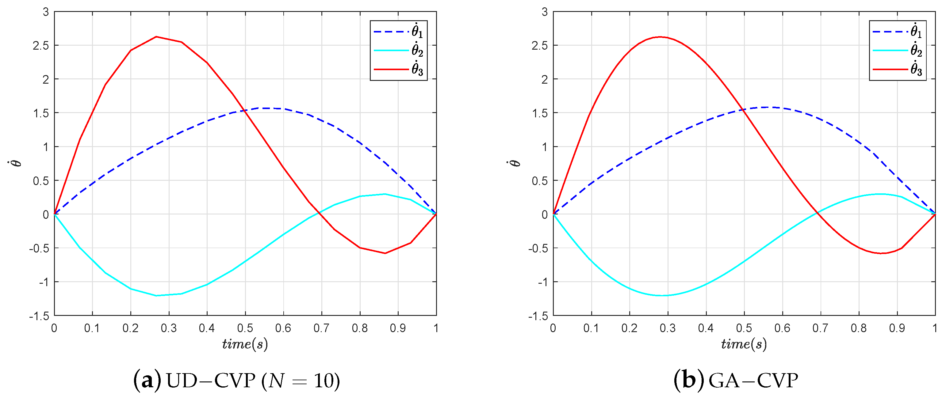
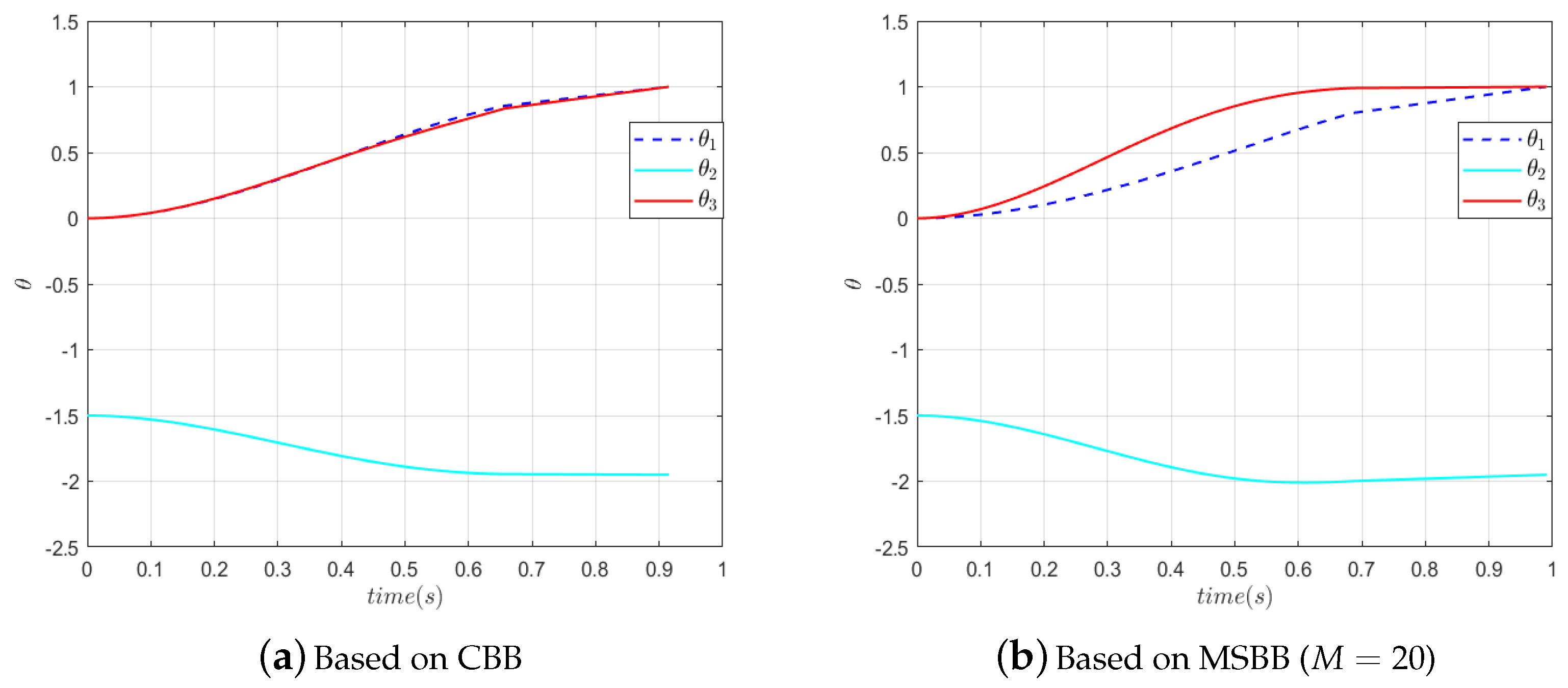
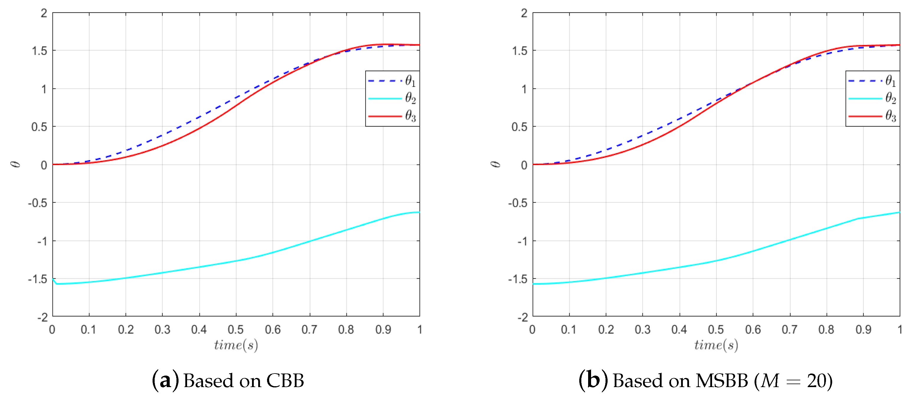
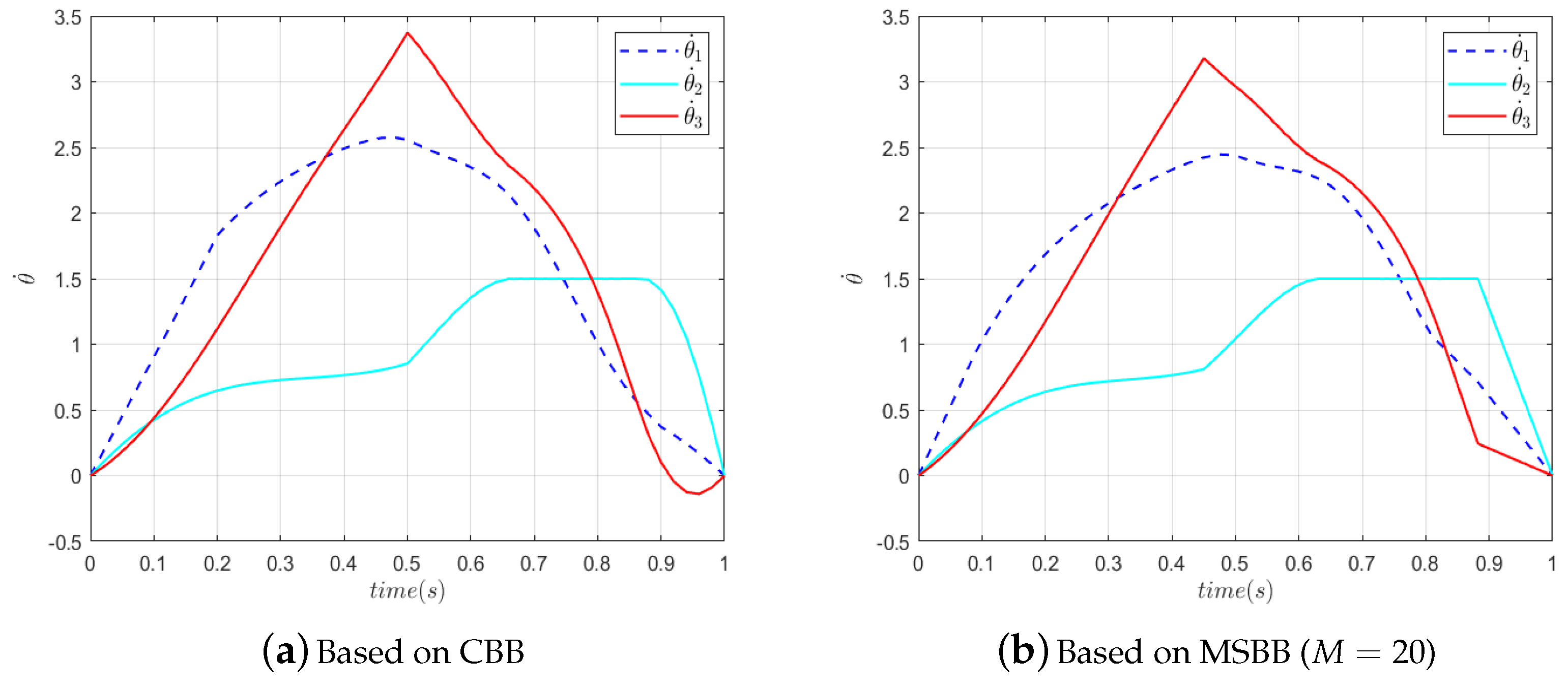
Except for the no-collision constraint, other constraints are shown in the Equation (16). Set the weighs ${\lambda }_1={\lambda }_2=0.5$. The collision-free OTP is solved by GA-CVP, and the simulation is carried out on MATLAB. Figure 10 and Figure 11 show the angular velocity for each joint angle during RA motion. Figure 12 and Figure 13 show the angular velocity for each joint angle during RA motion.

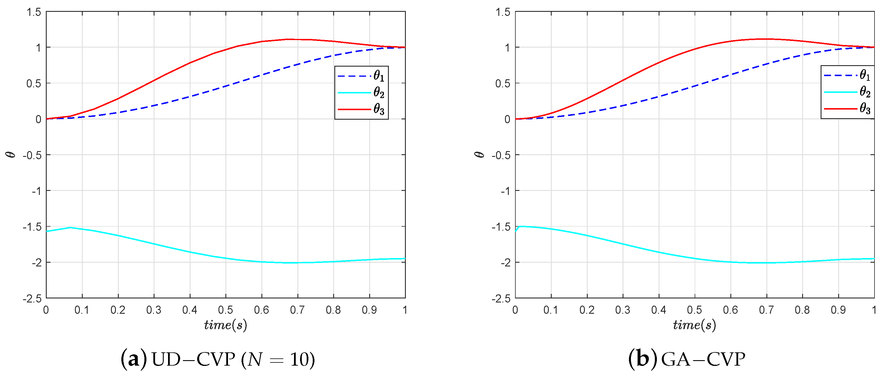
According to the four curves in Figure 10 and Figure 11, the joint angles at the initial and terminal moments of the RA meet the task requirements. The manipulator can move accurately from the initial position to the target position, and each joint rotation is within the range. It is clear that all four curves are smooth. This indicates that the joint angle changes smoothly and that there are no sudden changes in angle. It can be seen from Figure 12 and Figure 13 that the angular velocities of the joints are also within the velocity constraints. Both ${\dot{\theta }}_2$ in Figure 13a at $t\in [0.66,0.88]$ and ${\dot{\theta }}_2$ in Figure 13b at $t\in [0.63,0.882]$ reach their maximum angular velocity, indicating that they are constrained by their respective upper line of angular velocities during these periods.

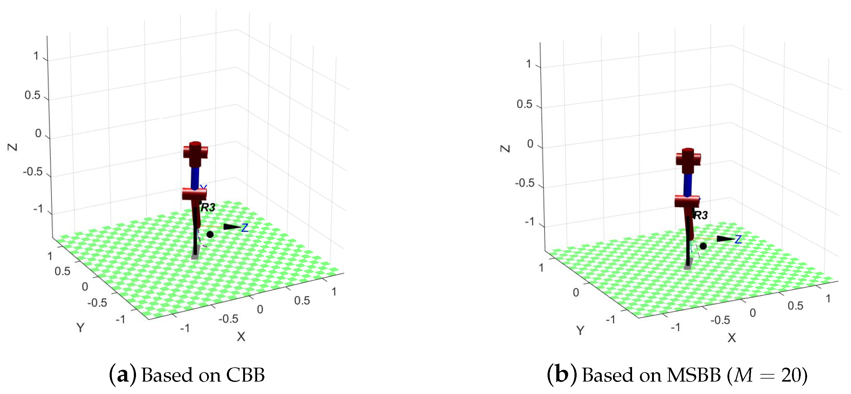
Figure 14 and Figure 15 show that the trajectory of the manipulator was simulated in MATLAB. Based on the four trajectories in Figure 14 and Figure 15, it can be seen that both the trajectories based on the CBB and MSBB are effective in avoiding obstacles. Moreover, the trajectory of the manipulator is smooth for different tasks. By comparing Figure 14a with Figure 14b, it can be seen that the trajectory planned based on MSBB is closer to the obstacle. The CD based on MSBB is more sensitive.

To further compare the CD sensitivity and computational complexity of the two bounding boxes, MSBB with a different number of spheres is used to envelop the link. When $M=5$, the minimum enclosing sphere radius $r_{O_{k_M}}$ of MSBB is slightly larger than the radius $r_3$ of the CBB, so the number of enclosing spheres M of MSBB is 20, 15, 10, 6, 5. Based on these conditions, we record the shortest distance $d_{min}$ between the manipulator and the obstacle and the calculation time for two different tasks.

Table 6. Angular velocity variation curve of each joint during robot motion (Task 1).

Collision Detection Method	Calculation Time/s	${\mathit{d}}_{min}/$m
CBB	325.8470	0.1320
MSBB ($M=20$)	712.4350	0.0779
MSBB ($M=15$)	477.6600	0.0811
MSBB ($M=10$)	415.4250	0.0922
MSBB ($M=6$)	309.3350	0.1230
MSBB ($M=5$)	220.7140	0.1411

and

Table 7. Angular velocity variation curve of each joint during robot motion (Task 2).

Collision Detection Method	Calculation Time/s	${\mathit{d}}_{min}/$m
CBB	262.0840	0.1920
MSBB ($M=20$)	542.6440	0.1220
MSBB ($M=15$)	467.9660	0.1401
MSBB ($M=10$)	301.3400	0.1444
MSBB ($M=6$)	175.8210	0.1894
MSBB ($M=5$)	141.1260	0.1947

show the results.

From Table 6 and Table 7, it is seen that the shortest distance is $d_{min}>0$ between the robot arm and the obstacle. It indicates that the collision-free trajectory can be successfully planned under both conditions of Task 1 and Task 2 based on the two different bounding boxes. When the number of enveloping spheres $M=20,15,10,6$ of MSBB, the shortest distance between the manipulator and the obstacle for both Task 1 and Task 2 is smaller than that based on the CBB. Therefore, MSBB is more sensitive when the minimum enclosing ball radius $r_{O_{k_M}}$ is smaller than the cylinder radius $r_3$. Moreover, in Task 1, the minimum distance based on MSBB ($M=20$) is nearly one half of the minimum distance based on the CBB. However, as the number of envelope spheres M increases, the calculation time also increases. In real-world applications, it is necessary to take into account the relation between the quantity of envelope spheres and the calculation time. Choose the appropriate number of envelope balls, the requirement of the shortest distance $d_{min}$ is met. The real-time requirement of movement is also met.

5. Conclusions

In this study, the approach combining non-uniform adaptive time grid and BBCD is used to solve the asymmetric collision-free OTP with comprehensive optimization goal of time and energy. First, based on the multi-sphere envelope RA, the collision detection is realized by using the spatial position relationship, Then, this relationship is used as the non-collision constraint in OTP. Secondly, according to the changing trend of the control vector, GA-CVP merges or inserts the original time nodes into the grid to form a new asymmetric time grid. After that, the OTP is transformed to the non-uniform discrete NLP problem. Finally, the NLP problem is solved with the new grid. Simulation experiments show that the approach proposed not only ensures the solution accuracy but also improves the solution efficiency, to obtain optimal trajectory from symmetric paths near the obstacles.

On the other hand, the proposed method is specifically applied to R3-RA, the generalizability of the approach to RA with different DOF or different type should be further studied. Moreover, the optimization of the solution process of differential equations is the focus of future work. When implemented in practice, a trade-off should be made between obstacle avoidance sensitivity and computation time, an appropriate number of enclosing spheres should be selected.

References

1. Zhang, C.; Wang, Y.; Ma, X.; Mu, C. Obstacle Avoidance Path Planning of Manipulator with Improved Artificial Potential Field Method. Modul. Mach. Tools Autom. Process. Technol. 2023, 4, 27–30. [Google Scholar]
2. Ekrem, O.; Aksoy, B. Trajectory Planning for a 6-axis Robotic Arm with Particle Swarm Optimization Algorithm. Eng. Appl. Artif. Intell. 2023, 122, 106099. [Google Scholar] [CrossRef]
3. Wang, L.; Wang, X.; Liu, G.; Sheng, Z. Preference-based Multi-Objective Shark Optimization Algorithm for Train Operation. J. Sci. Instrum. 2020, 41, 245–256. [Google Scholar]
4. Liu, P.; Liu, H.; Qiu, G.; Liu, X. Gauss Time Grid Parametric Trajectory Planning for Hypersonic Vehicle under Thermal Rate Constraint. Control Theory Appl. 2022, 39, 2283–2292. [Google Scholar]
5. Liu, P.; Li, G.; Yang, J.; Liu, X. Fast Numerical Algorithm for Optimal Control of Swing in Container Handling. Control Theory Appl. 2019, 36, 1275–1282. [Google Scholar]
6. Shi, B.; Yin, Y.; Liu, F. Optimal Feeding Control of Biochemical Reaction Process based on Non-Uniform Parameterization. In Proceedings of the 30th Chinese Process Control Conference (CPCC 2019) Abstract Set. Process Control Committee of the Chinese Society of Automation, Kunming, China, 1–2 August 2019; pp. 36–44. [Google Scholar]
7. Guo, H.; Mo, Y.; Zhang, Y. Orthogonal Design-based Control Vector Parameterization Combined with Improved Seagull Optimization Algorithm for Dynamic Optimization Problems. IEEE Access 2022, 10, 65238–65256. [Google Scholar] [CrossRef]
8. Zhou, M.; Zhang, X. Fast Collision Checking for Dual-Arm Collaborative Robots Working in Close Proximity. In Proceedings of the 2022 International Conference on Robotics and Automation (ICRA), Philadelphia, PA, USA, 23–27 May 2022; pp. 243–249. [Google Scholar]
9. Zhao, H.; Lei, C.; Jiang, N. Path Planning of 6-DOF Manipulator based on Improved Ant Colony Algorithm. J. Zhengzhou Univ. (Sci.) 2020, 52, 120–126. [Google Scholar]
10. Hou, D.; Wang, X.; Liu, J.; Yang, B.; Hou, G. Research on Collision Avoidance Technology of Manipulator based on AABB Hierarchical Bounding Box Algorithm. In Proceedings of the 5th Asian Conference on Artificial Intelligence Technology (ACAIT), Haikou, China, 29–31 October 2021; pp. 406–409. [Google Scholar]
11. Yang, F. AABB Bounding Box Collision Detection Algorithm based on B+ Tree Storage. Comput. Sci. 2021, 48, 331–333. [Google Scholar]
12. Fu, Z.; Yu, Q.; Xiong, P.; Wang, Z.; Zhao, Z. Simulation of Manipulator Path Planning based on Improved Artificial Potential Field Method. Mach. Tool Hydraul. 2021, 49, 20–24. [Google Scholar]
13. Wang, X.; Wang, T.; Ding, W. Manipulator Path Planning based on Improved Artificial Potential Field Method. Comb. Mach. Tool Autom. Mach. Technol. 2022, 06, 24–27. [Google Scholar]
14. Gan, B.; Dong, Q. An Improved Optimal Algorithm for Collision Detection of Hybrid Hierarchical Bounding Box. Evol. Intell. 2022, 15, 2515–2527. [Google Scholar] [CrossRef]
15. Zhu, Z.; Jing, S.; Zhong, J.; Wang, M. Obstacle Avoidance Path Planning of Space Redundant Manipulator based on a Collision Detection Algorithm. Xibei Gongye Daxue Xuebao/J. Northwestern Polytech. Univ. 2020, 38, 183–190. [Google Scholar] [CrossRef]
16. Zhang, S.; Dai, S.; Zanchettin, A.M.; Villa, R. Trajectory Planning based on Non-Convex Global Optimization for Serial Manipulators. Appl. Math. Model. 2020, 84, 89–105. [Google Scholar] [CrossRef]
17. Verstraten, T.; Schumacher, C.; Furnémont, R.; Seyfarth, A.; Beckerle, P. Redundancy in Biology and Robotics: Potential of Kinematic Redundancy and its Interplay with Elasticity. J. Bionic Eng. 2020, 17, 695–707. [Google Scholar] [CrossRef]
18. Qiao, P.; Wu, Y.; Ding, J. Optimal Control of a Black-Box System based on Surrogate Models by Spatial Adaptive Partitioning Method. ISA Trans. 2020, 100, 63–73. [Google Scholar] [CrossRef] [PubMed]
19. Christ, F.; Wischnewski, A.; Heilmeier, A.; Lohmann, B. Time-Optimal Trajectory Planning for a Race Car Considering Variable Tyre-Road Friction Coefficients. Veh. Syst. Dyn. 2021, 59, 588–612. [Google Scholar] [CrossRef]
20. Li, X.; Gu, Y.; Wu, L.; Sun, Q.; Song, T. Time and Energy Optimal Trajectory Planning of Wheeled Mobile Dual-Arm Robot based on Tip-Over Stability Constraint. Appl. Sci. 2023, 13, 3780. [Google Scholar] [CrossRef]
21. Sang, W.; Sun, N.; Zhang, C.; Qiu, Z.; Fang, Y. Hybrid Time-Energy Optimal Trajectory Planning for Robot Manipulators with Path and Uniform Velocity Constraints. In Proceedings of the 2022 13th Asian Control Conference (ASCC), Jeju Island, Republic of Korea, 4–7 May 2022; pp. 334–340. [Google Scholar]
22. Xu, W.; Jiang, A.; Jiang, E.; Zhang, Q. A Fast and Efficient Control Vector Parameterization Optimization Method. J. Hangzhou Dianzi Univ. (Nat. Sci.) 2019, 39, 40–46. [Google Scholar]
23. Wu, D.; Chen, Y.; Yu, C.; Bai, Y.; Teo, K.L. Control Parameterization Approach to Time-Delay Optimal Control Problems: A survey. J. Ind. Manag. Optim. 2023, 19, 3750–3783. [Google Scholar] [CrossRef]
24. Chen, X.; You, X.; Jiang, J.; Ye, J.; Wu, H. Trajectory Planning of Dual-Robot Cooperative Assembly. Machines 2022, 10, 689. [Google Scholar] [CrossRef]
25. Rösmann, C.; Makarow, A.; Bertram, T. Online Motion Planning based on Nonlinear Model Predictive Control with Non-Euclidean Rotation Groups. In Proceedings of the 2021 European Control Conference (ECC), Delft, The Netherlands, 29 June–2 July 2021; IEEE: Piscataway, NJ, USA; pp. 1583–1590. [Google Scholar]
Figure 1. The three DOF industrial RA.
Symmetry 15 01155 g001
Figure 2. Schematic diagram of grid reconfiguration strategy.
Symmetry 15 01155 g002
Figure 3. Information on the left and right slopes of time nodes t j , i .
Symmetry 15 01155 g003
Figure 4. GA-CVP algorithm flow chart.
Symmetry 15 01155 g004
Figure 5. Angle change curve of each joint ( λ 1 = λ 2 = 0.5 ).
Symmetry 15 01155 g005
Figure 6. Angular velocity variation curve of each joint ( λ 1 = λ 2 = 0.5 ).
Symmetry 15 01155 g006
Figure 7. Simplified schematic diagram of robot and obstacle model.
Symmetry 15 01155 g007
Figure 8. Sphere position diagram.
Symmetry 15 01155 g008
Figure 9. Simplified schematic diagram of the manipulator model.
Symmetry 15 01155 g009
Figure 10. Curve of the change in the angle of each joint during robot movement (Task 1).
Symmetry 15 01155 g010
Figure 11. Curve of the change in the angle of each joint during robot movement (Task 2).
Symmetry 15 01155 g011
Figure 12. Angular velocity variation curve for each joint during robot motion (Task 1).
Symmetry 15 01155 g012
Figure 13. Angular velocity variation curve for each joint during robot motion (Task 2).
Symmetry 15 01155 g013
Figure 14. Robot end trajectory diagram (Task 1).
Symmetry 15 01155 g014
Figure 15. Robot end trajectory diagram (Task 2).
Symmetry 15 01155 g015