Article

Ollivier–Ricci Curvature Based Spatio-Temporal Graph Neural Networks for Traffic Flow Forecasting

1
School of Geosciences and Info-Physics, Central South University, Changsha 410083, China
2
College of Automotive and Mechanical Engineering, Changsha University of Science & Technology, Changsha 410114, China
3
School of Geographical Sciences, Hunan Normal University, Changsha 410083, China
4
The 27th Research Institute, China Electronic Technology Group Corporation, Zhengzhou 450047, China
*
Author to whom correspondence should be addressed.
Symmetry 2023, 15(5), 995; https://doi.org/10.3390/sym15050995
Submission received: 6 March 2023 / Revised: 10 April 2023 / Accepted: 25 April 2023 / Published: 27 April 2023
(This article belongs to the Special Issue Machine Learning and Data Analysis)

Abstract

:
Traffic flow forecasting is a basic function of intelligent transportation systems, and the accuracy of prediction is of great significance for traffic management and urban planning. The main difficulty of traffic flow predictions is that there is complex underlying spatiotemporal dependence in traffic flow; thus, the existing spatiotemporal graph neural network (STGNN) models need to model both temporal dependence and spatial dependence. Graph neural networks (GNNs) are adopted to capture the spatial dependence in traffic flow, which can model the symmetric or asymmetric spatial relations between nodes in the traffic network. The transmission process of traffic features in GNNs is guided by the node-to-node relationship (e.g., adjacency or spatial distance) between nodes, ignoring the spatial dependence caused by local topological constraints in the road network. To further consider the influence of local topology on the spatial dependence of road networks, in this paper, we introduce Ollivier–Ricci curvature information between connected edges in the road network, which is based on optimal transport theory and makes comprehensive use of the neighborhood-to-neighborhood relationship to guide the transmission process of traffic features between nodes in STGNNs. Experiments on real-world traffic datasets show that the models with Ollivier–Ricci curvature information outperforms those based on only node-to-node relationships between nodes by ten percent on average in the RMSE metric. This study indicates that by utilizing complex topological features in road networks, spatial dependence can be captured more sufficiently, further improving the predictive ability of traffic forecasting models.

1. Introduction

Intelligent transportation system (ITS) is an important component of smart cities, and they have the potential to contribute to the operational efficiency of urban systems and rationalization of decision-making. Traffic flow forecasting is one of the fundamental functions required for ITS, which aims to predict the future traffic flow features of urban transportation systems (e.g., traffic flow, vehicle density, speed, and passenger demand) using historical traffic observation data. Accurate traffic prediction results can help optimize urban traffic scheduling and management and provide convenience to citizens. However, traffic flow forecasting has long been considered challenging because of the complex spatiotemporal dependence on traffic flows. The complex spatiotemporal dependence in traffic flow is reflected in two aspects: on the one hand, different nodes on the road network are intricately spatial dependent, and both neighboring nodes and the geographically distant but close interacting nodes can influence the traffic flow of the target node; on the other hand, there is a complex nonlinear correlation among historical traffic observation data.
With the development of deep learning, researchers have conducted extensive studies on deep learning models for traffic flow forecasting tasks in recent years, such as modeling the spatial dependence among traffic nodes by convolutional neural networks (CNNs) [1] or graph neural networks (GNNs) [2]; capturing the temporal dependence between the traffic flow of nodes at future moments and historical observations by CNN or recurrent neural networks (RNNs); and obtaining spatiotemporal features that can be used to predict the future traffic conditions by combining temporal and spatial features learned from historical data. Regarding spatial dependence modeling, current mainstream traffic flow forecasting models use graph neural networks to model spatial dependence because CNN architecture does not match traffic network data with complex topologies, while GNNs can model graph data more naturally. Most graph neural networks are effective in modeling graph data because their message passing mechanism [3] enables graph neural networks to predict the traffic feature of a single node using traffic information of local or global nodes, so these graph neural networks are also called message passing neural networks (MPNNs).
For traffic flow forecasting, the message-passing mechanism of graph neural networks is the key to modeling the spatial dependence of road network nodes. The graph structure which guides the message-passing process can represent the spatial dependence in the road network, and how to model the spatial dependence and construct the graph structure has long been a research topic. The existing traffic forecasting methods based on the road network graph structure for message passing are mainly based on the node-to-node relations between nodes (e.g., node adjacency on the road network, the spatial distance between nodes) to guide the message passing process of GNNs, and the underlying assumption is that the neighboring nodes on the road network share the similar traffic pattern or the closer nodes have stronger traffic connections. The mechanism of adjacency graph-based message passing is shown in Figure 1a, where features of neighboring nodes are assigned equal weights in the process of feature aggregating [4,5,6]; the mechanism of spatial distance graph-based message passing is shown in Figure 1b, where the relationship between weight and distance is usually determined by a Gaussian kernel function (i.e., the aggregation weight to neighboring nodes is inversely proportional to the square of spatial distance) [7,8,9].
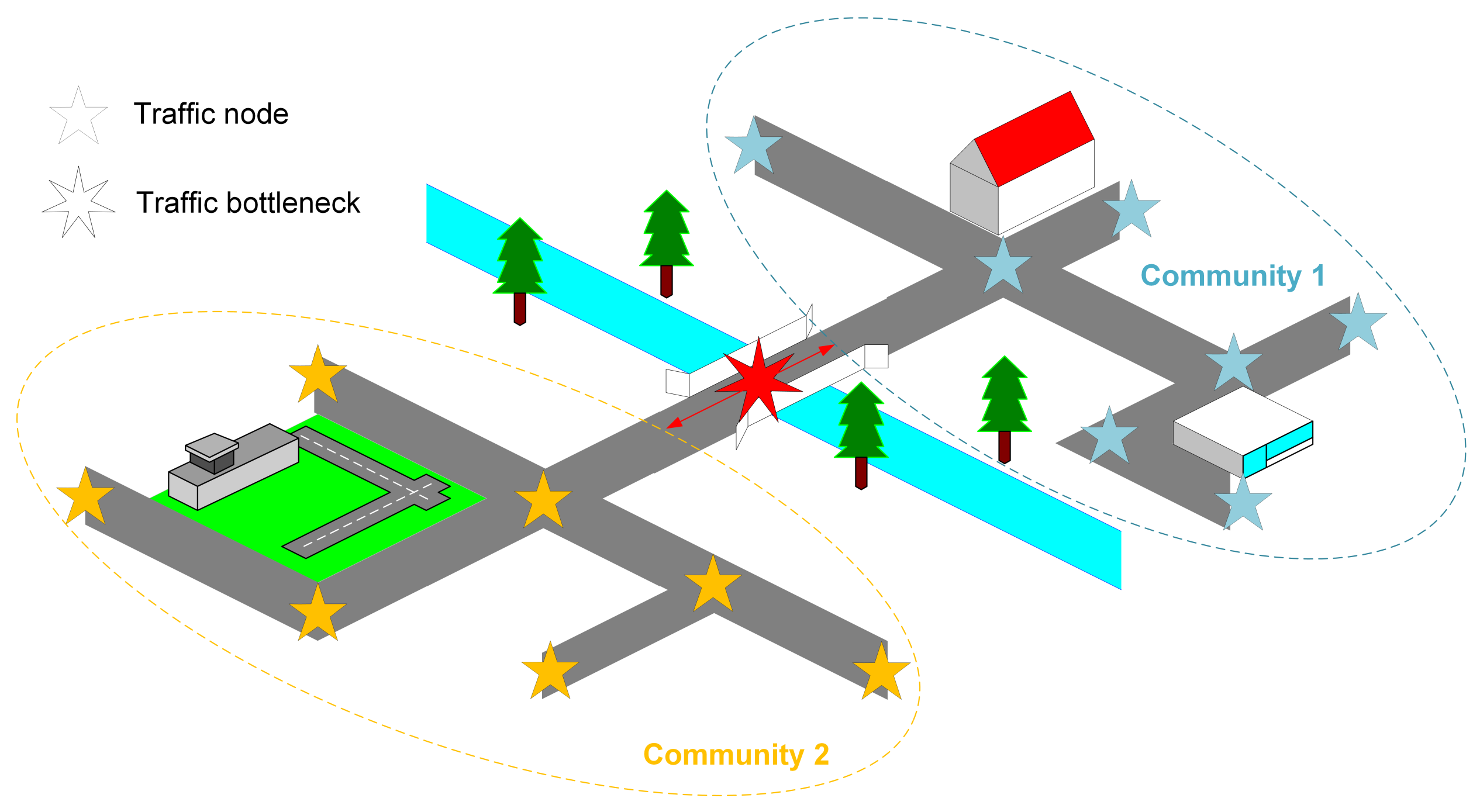
Most existing methods that consider the topology of the road network are only concerned with adjacency relations, which only consider simple node-to-node relations and neglect the interactions between communities in the road network. However, we argue that the Ollivier–Ricci curvature [10], as an intrinsic topological property of the road network, has a large impact on the traffic flow and can be used to measure the influence of the neighborhood-to-neighborhood relationships between nodes on the spatial dependence. Bottleneck edges are of great importance for the interactions between communities, and Ollivier–Ricci curvature can be used to measure the bottleneck degree of edges in a road network. As shown in Figure 2, traffic transmission between nodes in different regions is often carried by a few bottleneck edges with high negative curvature in the local network (e.g., the bridge in Figure 2), and “bottleneck” means the neighborhoods of the nodes at both ends of the edge tend to pass through this edge to interact with each other. The more bottleneck, the greater impact on the traffic flow of each other for two nodes connected by this bottleneck edge. The edges with positive curvatures, on the other hand, connect the nodes within the same community and are not likely to be bottlenecks in the road network.
In this paper, we conduct experiments on several real-world traffic datasets to verify whether applying Ollivier–Ricci curvature information to guide the message passing process of the STGNNs model can improve traffic forecasting performance, and the results show that Ollivier–Ricci curvature information is fertile for the traffic flow forecasting ability of STGNNs. The main contributions of this paper are as follows:
  • We introduce an edge bottleneck coefficient based on the Ollivier–Ricci curvature to measure the bottleneck coefficient of edges in the road network and take the neighborhood-to-neighborhood connectivity into consideration.
  • We design a curvature graph convolution module to utilize this coefficient to guide the message-passing process of STGNNs and enhance their ability to capture the spatial dependence of road network nodes.
  • Experiments conducted on two real-world traffic prediction benchmark datasets show that the proposed enhancement strategy for STGNNs based on Ollivier–Ricci curvature is effective.
The rest of the paper is organized as follows: Section 2 summarizes the work related to the traffic flow forecasting model and the design of the road network graph structure; Section 3 depicts the details of the method proposed in this paper; Section 4 presents the experiments conducted in this paper, including the validation of the proposed method on a real-world road network traffic datasets; and Section 5 concludes the whole paper.

2. Related Work

2.1. Deep Learning-Based Traffic Forecasting Methods

In recent years, due to the achievements of deep learning in many challenging and complex learning tasks [11], much attention has been paid to deep learning, and numerous deep learning-based traffic prediction methods have been proposed since. Novel deep neural network architectures are designed to capture complex patterns in historical traffic flow sequences, including spatiotemporal dependence and the influence of external environmental factors on traffic flow.
To model temporal dependence, early approaches mainly adopt recurrent neural network-based methods, including long short-term memory (LSTM) networks and gated recurrent units (GRU). However, RNN-based models are greatly constrained by the problem of gradient vanishing, making them less friendly to learn from longer sequences. In response to the shortcomings of RNN-based models, researchers utilize convolutional neural networks (CNNs) to model traffic flow. For example, dilated convolution [12] is used to model long-range temporal characteristics.
To model spatial dependence, many researchers initially employ CNNs to model the correlations between geographic units. Traffic flow prediction models capable of capturing complex spatiotemporal patterns are formed through the fusion of multiple network architectures. For example, Zhang et al. propose an ST-ResNet [13], which designs a residual convolutional network for each attribute of temporal closeness, periodicity, and trend of crowd flow. Then the outputs of the three networks are aggregated with external factors to predict the inflow and outflow of crowds in each region of the city. The main problem with ST-ResNet is that it simply combines spatial dependence with three different time periods. Ali et al. further propose an AAtt-DHSTNet [14], which can simultaneously capture the spatiotemporal correlation in crowd flow data. Although the introduction of CNNs to model spatial dependence among urban units has substantially advanced the progress of traffic forecasting research, CNNs themselves are not well suited to traffic networks with complex topologies. In other words, adopting CNNs to model spatial dependence of road networks is not natural.
In recent years, with the proposal of graph neural networks (GNNs), many methods for graph-related tasks have emerged [15,16,17]. For traffic forecasting tasks, GNNs allow us to model the spatial dependence of road networks more naturally, and methods based on GNNs to model the spatial dependence of traffic flow have achieved great success in recent years. Such methods are collectively referred to as spatiotemporal graph neural networks (STGNNs) in this paper. T-GCN [18] models the spatiotemporal dependence of traffic flow by fusing GRU and GCN but fails to consider the influence of external factors on the traffic system. Based on T-GCN, KST-GCN [19] is further proposed, which adopts knowledge graphs to take the effect of external factors on traffic systems into consideration. Similarly, GCN-DHSTNet [20] incorporates external factors with the GCN-LSTM network. However, as RNN-based models, both KST-GCN and GCN-DHSTNet face the problems of long training time and difficulty in capturing long-range temporal dependence. Yu et al. propose an STGCN [21] that adopts GCN to capture the spatial dependence in traffic flow and combines with one-dimensional convolution to capture the temporal dependence, but the ordinary one-dimensional convolution in STGCN needs to be stacked in multiple layers to capture the long-range dependence effectively. Therefore, Graph WaveNet [22] applies a dilated one-dimensional convolution to overcome this issue.

2.2. Spatial Dependence Graph Construction

The key to capturing the spatial dependence of the traffic flow of GNNs lies in their message-passing mechanism. As shown in Figure 3, features between nodes in the road networks are passed to neighboring nodes, and traffic features from neighboring nodes are aggregated, thus, enabling the model to utilize the historical features from both the neighbors and the node itself to predict the future traffic conditions of a node. As a way to model spatial dependence, how to construct the graph structures that message passing in STGNNs rely on has long been a research topic in the field of traffic flow forecasting. Some research measures the spatial dependence between nodes by their temporal similarity or functional similarity [23,24,25]. For example, T-MGCN [23] uses the DTW algorithm to calculate the similarity of temporal patterns and utilizes POI information to measure the functional similarity between nodes but ignores the impact of road network structure on the spatial dependence between nodes. Other work constructs spatial dependence graphs based on the topological structure of the road network or the spatial relations in the road network [4,5,7,8]. Most STGNNs utilize the distance-based spatial dependence graph [7,18,21], in which distant nodes are less related to each other, while some other work considers intersecting roads to be associated [4,5]. However, these methods only consider simple adjacency relations or distance information without digging deeper into the essential topological characteristics, while topological characteristics of the road network, such as curvature, can have a certain impact on traffic flow.

2.3. Connection between Discrete Ricci Curvature and Network Properties

Ricci curvature is a measure of the degree to which a manifold deviates locally from Euclidean space in Riemannian geometry, and it is closely related to the properties of manifolds and can be used as a powerful tool to solve many problems in differential geometry [26]. Many researchers have explored how to migrate Ricci curvature in continuous spaces to discrete spaces (e.g., networks) and have conducted studies on the relation between the average transport distance and discrete Ricci curvature. Ollivier considers the relation between the transport distance between nodes and the average transport distance between neighbors of nodes and defines the Ollivier–Ricci curvature [10] based on the optimal transport theory. Numerous works show that Ollivier–Ricci curvature can be used to reveal the community structures in complex networks [27], the fragility of road network topology [28], the supply-demand mismatch in transportation networks [29], and the network congestion phenomenon [30], etc. Forman defines the Forman–Ricci curvature [31] based on the theoretical framework of CW complex, which can be applied to such fields as network clustering, network extrapolation [32], and image processing [33].

3. Methodology

3.1. Problem Definition

The goal of traffic flow forecasting is to predict the future traffic flow of the road network, given the historical traffic flow. The task can be formalized as a multivariate time series forecasting problem with additional prior knowledge. For an STGNN, the graph structure G for subsequent message passing is the a priori knowledge about the spatial dependence of nodes in the network.
Definition 1 
(Graph structure of traffic network G). In this paper, we use G ( V , E , A ) to represent the road network structure, where V denotes the set of nodes representing different locations (e.g., road sections, sensors) in the road network, E denotes the set of connected edges between nodes, and A is the adjacency matrix indicating the node-to-node relations (e.g., adjacency, geographic distance, similarity, etc.) between nodes. N ( i ) denotes the set of neighbors of node i.
Definition 2 
(Traffic flow features tensor X N × F × T ). The traffic flow of nodes in the road network at each sample time is the feature of nodes. N represents the size of the node set | V | , F denotes the number of traffic features such as speed and flow. F is 1 if the prediction is based on the speed of traffic flow only. T is the number of sample times.
Definition 3 
(Traffic forecasting task). As shown in Equation (1), the traffic forecasting task can be formalized as predicting the traffic flow features tensor in Q future time steps given the graph structure G and the historical traffic flow features of P time steps.
X t + 1 , X t + 2 , , X t + Q = f G ; X t P , , X t 1 , X t

3.2. Ollivier–Ricci Curvature of Graphs

The Ollivier–Ricci curvature is defined based on the optimal transport theory. The problem of optimal transport was first proposed by G. Monge, and it can be formulated figuratively as finding the transport solution corresponding to the minimum amount of work required to move a pile of sand from one location to another and to give the pile a specific shape. If the sand pile in the above example is considered a probability distribution, and the process of moving the sand pile is considered a transformation between probability distributions, the “minimum work” corresponding to the optimal transport solution is equivalent to the distance between probability distributions. Then the problem of optimal transport can be expressed formally as follows: given a source distribution space X and a target distribution Y, the cost of transmitting a unit mass from position x in X to position y in Y is c ( x , y ) , and the problem is to solve a probability distribution transformation scheme T : X Y such that the cost of transforming X to Y is minimized. The minimum transport cost has different representations in different application scenarios. For example, Kantorovich relaxes the optimal transport problem and proposes that the transport process is not necessarily deterministic (the mass in a source can only be transported to a target) but can be probabilistic (the mass in one location can be distributed to multiple other locations) [34]. Given the probability distributions m i and m j at given points i and j, the distance between m i and m j can be expressed as Equation (2):
W 1 m i , m j = inf μ i , j m i , m j i , j V × V d i , j μ i , j i , j
The distance W 1 m i , m j is called Wasserstein-1 distance, where μ i , j is the mass that needs to be transmitted from point to point when transforming m i to m j ; d i , j denotes the metric, for example, the distance between two nodes; ( m i , m j ) represents the set of all joint distributions with m i and m j as marginal distributions, and satisfies the following relations in Equation (3):
j V μ i , j i , j = m i i , i V μ i , j i , j = m j j
Equation (3) represents the probability of all possible mass transport processes that start with m i and end with m j . As a measure between probability distribution, Wasserstein-1 distance has been successfully applied in computer vision [35], natural language processing [36], and other fields. It can also be used as a distance measure between node neighborhoods in graphs to help recognize patterns in complex networks. For example, for unweighted graphs, a smaller Wasserstein-1 distance between two nodes indicates that there are more overlapping nodes between the neighborhoods of these two nodes.
The Ollivier–Ricci curvature of edge i j E between node i and node j considers the node-to-node distance between i and j and the neighborhood-to-neighborhood distance, i.e., Wasserstein-1 distance, and its definition is shown in Equation (4):
κ i j = 1 W 1 m i , m j d i , j
With this definition, now we consider the connection between Ollivier–Ricci curvature and the local topological characteristics of road networks. Suppose node i and node j are two nodes in a road network; if node i and node j are in different communities, then their neighborhoods have few overlapping nodes, and the transport from m i , the neighborhood of node i, to m j , the neighborhood of node j, is more dependent on the path i j . As W 1 m i , m j > d i , j , the curvature of i j is negative. If node i and node j are in the same community, then their neighborhoods have many overlapping nodes, and then the transport from m i to m j is less dependent on the path i j and can be finished via multiple paths between neighbor nodes. As W 1 m i , m j < d i , j , the curvature of edge i j is now positive.
In the formula of Ollivier–Ricci curvature, the probability distribution function of the neighborhood of node i V needs to be defined explicitly. In this paper, we choose a commonly adopted empirical family of probability distribution [27]:
m i α , p ( x ) = α if x = α 1 α C · exp d ( i , x ) p if x N ( i ) 0 otherwise
where hyperparameter α [ 0 , 1 ] is used to control the weight of information between the node itself and its neighboring nodes; the hyperparameter p is used to control the distance effect between nodes. In particular, when p = 0 , m i α , 0 x = 1 α | N i | , x N i is a uniform distribution, and the distances between nodes do not affect the probability distribution of neighborhood. C = x i exp ( ( d i , x ) p ) denotes the normalization factor.

3.3. Curvature Enhanced Graph Neural Networks

3.3.1. Edge Bottleneck Coefficients

As shown in Figure 4, the edges with negative curvature in the network tend to connect different locally connected communities; and the edges with positive curvature tend to connect nodes in the same community. Since the interaction between nodes in different communities is more dependent on the edges with negative curvature in the local topology of the road network, and the interaction between nodes in the same community relies on the edges with positive curvature, the value of Ollivier–Ricci curvature can be used to represent the level of bottleneck for edges in the local network to guide the message passing between nodes in STGNNs and enhance the ability to capture the spatial dependence of road network.
Although the positive and the negative signs of Ollivier–Ricci curvature are indicative of the local topological structure of the network, the direct application of the raw curvature values as weights for message aggregation is not conducive to model training [37]. In this paper, the edge curvature is normalized so that the obtained edge bottleneck coefficients r i j [ 0 , 1 ] are interpretable without having a significant impact on the convergence of the models. As shown in Equation (6), an edge with negative curvature corresponds to a larger r i j , indicating that the edge connects two communities in the local topological structure of the road network; an edge with positive curvature corresponds to a smaller r i j , indicating that the two nodes connected by the edge tend to be located in the same community.
r i j = 1 1 1 + e κ i j

3.3.2. Curvature Graph Convolution Module

Most graph neural networks can be classified as message-passing neural networks [38], which enable nodes to aggregate information from neighboring nodes and update their own features. Therefore, the node attributes can be predicted based on the features of the current node and its neighboring nodes, which is the reason why traffic forecasting models based on STGNNs can exploit the spatial dependence between nodes. The feature update process in the message passing mechanism can be expressed as Equation (7):
h i l + 1 = σ Φ j N ¯ i ( τ i j a i j W l + 1 h i l )
where h i l denotes the hidden features of node i in the l-th layer; N ¯ i = N i i is the union of the neighbors of node i and the node itself; Φ j N ¯ i ( ) denotes the aggregate function for aggregating the features from neighboring nodes, some examples are s u m ( ) , m a x ( ) and a v g ( ) ; a i j represents the strength of the connection between node i and node j; τ i j denotes the normalization coefficient, which considers the effect of the number of neighboring nodes on feature aggregation and ensures the numerical stability of the model during training. Generally, τ i j = 1 d i d j , where d i = j N ¯ i a i j is the degree of node i when considering self-loop. σ ( ) denotes the non-linear activation function, such as s i g m o i d ( ) , r e l u ( ) and t a n h ( ) .
We select the widely used s u m ( ) function as the aggregation function, r e l u ( ) as the nonlinear activation function, and introduce the edge bottleneck coefficient r i j to the message passing process, which can measure the influence of the neighborhood-to-neighborhood structure on the spatial dependence between nodes. In this way, the model can utilize the local topological information of the road network to guide the message-passing process. The message passing process of the curvature graph convolution module is shown in Equation (8):
h i l + 1 = σ j N ¯ i τ i j r i j a i j W l + 1 h i l )

3.3.3. Loss Function

In this paper, we adopt mean squared error (MSE) as the training objective of traffic prediction models. To predict the traffic flow of each node in Q future time steps given historical data of P time steps, the loss function can be defined as Equation (9).
L o s s W θ = i = t + 1 i = t + Q X : , i X : , i 2
where W θ represents learnable parameters in the model, X : , i denotes the ground truth of the traffic flow at time step i, and X : , i denotes the prediction of the traffic flow at time step i.

4. Experiments

4.1. Data Description

To verify the effectiveness of the Ollivier–Ricci curvature-based message aggregation strategy, experiments are conducted on two real-world traffic datasets, covering traffic speed prediction and traffic flow prediction tasks. The basic information of the datasets is shown in Table 1.
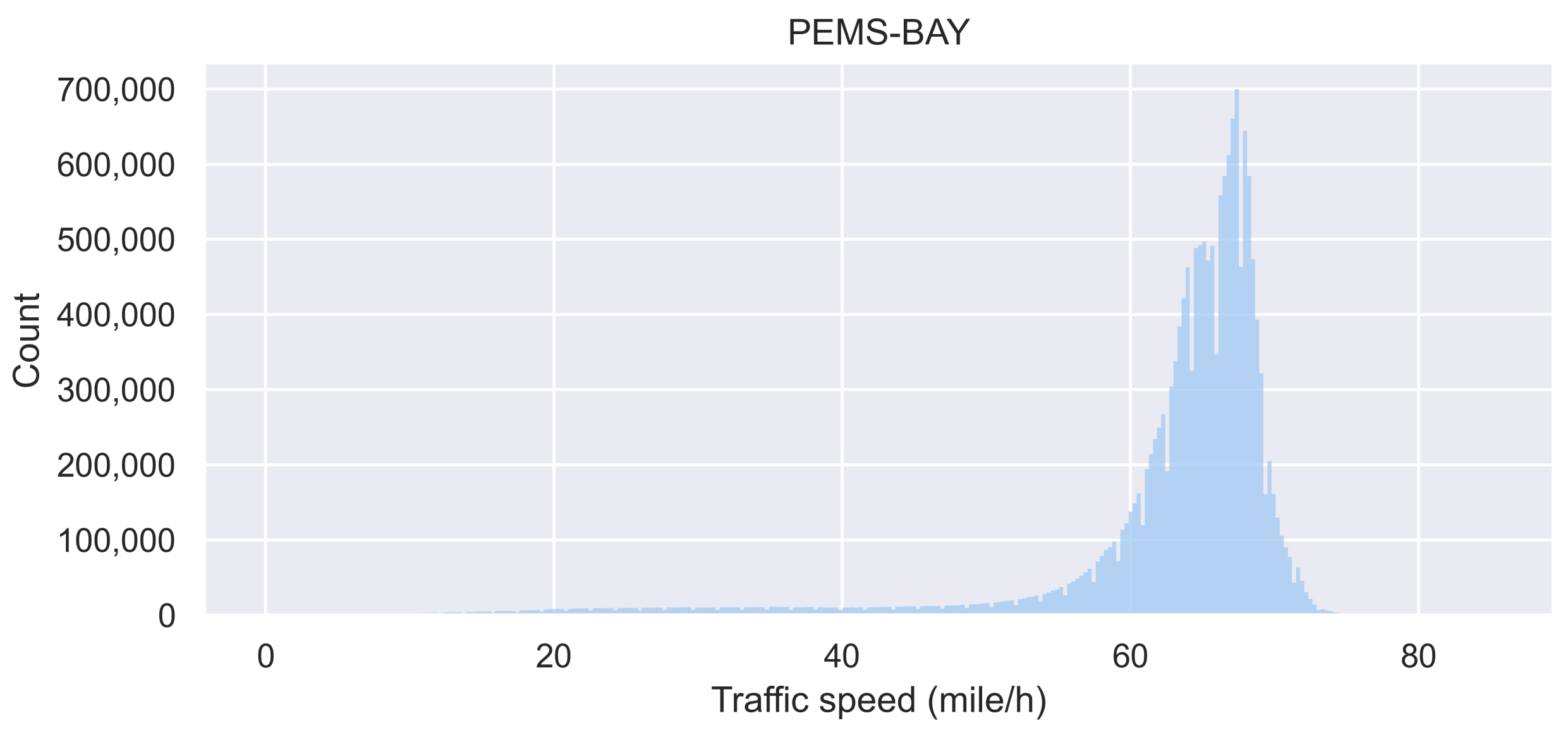
  • PEMS–BAY. PEMS–BAY dataset is a traffic speed dataset collected by California Transportation Agencies (CalTrans), containing the traffic speed data from 1 January 2017 to 30 June 2017, collected from 325 sensors. The data distribution is shown in Figure 5.
  • PEMSD7. PEMSD7 dataset contains traffic flow data collected by 883 sensors in District 7 of California from 1 July 2016 to 31 August 2016. The data distribution is shown in Figure 6.

4.2. Backbone Models and Evaluation Metrics

4.2.1. Backbone Models

We select STGNNs that only consider using road network structures such as distance graphs or adjacency graphs as baselines to fairly and intuitively evaluate the improvement brought by introducing curvature graphs. Backbone models that meet the above criteria are listed as follows:
  • STGCN [21]
    In STGCN, the spatial dependence of traffic data is modeled by GCN, where the graph for message propagation is constructed based on the spatial distance between nodes. The temporal dependence is modeled by a 1D convolutional neural network.
  • T-GCN [18]
    T-GCN adopts GCN and GRU to model spatial dependence and temporal dependence, respectively. The graph for message propagation is constructed based on spatial distances.

4.2.2. Comparison Setup

To evaluate the effectiveness of incorporating local topology for capturing the spatial dependence of road networks, we obtain the model to be validated (labeled as Backbone+) by replacing the graph convolution module with the curvature graph convolution module proposed in this paper. Meanwhile, to further investigate the influence of spatial distance on traffic prediction, we replace the graph convolution module with the adjacency graph convolution module, which retains only adjacency relations, i.e., the adjacency matrix contains only ones and zeros. The models with adjacency graphs are labeled as Backbone–. The three kinds of graphs are illustrated in Figure 7, and the specific comparison setup is shown in Table 2.

4.2.3. Evaluation Metrics

To quantitatively evaluate the performance of STGNNs with curvature-based graph convolution module and the original backbones, we select three common evaluation metrics to measure the difference between the prediction given by the model and the ground truth:
  • Mean absolute error (MAE):
    MAE = 1 n i = 1 n Y i Y i
  • Mean absolute percentage error (MAPE):
    MAPE = 1 n i = 1 n Y i Y i Y i × 100 %
  • Root mean squared error (RMSE):
    RMSE = 1 n i = 1 n Y i Y i 2

4.3. Experimental Setup

We conduct the following experiments based on the open source deep learning framework PyTorch [39], the traffic prediction framework LibCity [40], and the discrete Ricci curvature open source library GraphRicciCurvature [27], using an NVIDIA GeForce RTX 3060 GPU to train the models. Details of the experimental setup for the model training, input data preprocessing, and data splitting are described below.

4.3.1. Data Splitting

We split the original traffic dataset into the training set, validation set, and test set according to the time period, and the split ratio is 0.7/0.1/0.2. The traffic data in the first 70% time period of the dataset is used as the training set, the data in the 70% to 80% time period is used as the validation set, and the data in the last 20% is used as the test set.

4.3.2. Data Preprocessing

  • Distance-based message passing (node-to-node graph structure) 
    For models using spatial distance information to guide message passing, to ensure the numerical stability of the training process, the distances between nodes are mapped to distance correlation indices by a Gaussian kernel as shown in Equation (13).
    a i j = exp d i j 2 σ 2 , i j and exp d i j 2 σ 2 ϵ 1 , i = j 0 , otherwise .
  • Curvature-based message passing (neighborhood-to-neighborhood graph structure)
    To ensure the computational efficiency of message passing and lower the sparsity of the edge curvature matrix R, we mask R according to the sparse distance-based graph, i.e., only the curvature information of the connected edges of the closer nodes is considered. The mask matrix M is defined as Equation (14).
    M i j = 1 , a i j > 0 0 , a i j 0
    The mask operation to the edge curvature matrix R is shown as Equation (16).
    R = R M a s k
    where R = r i j , and ⨀ denotes Hadamard product.

4.3.3. Hyperparameter Settings

The hyperparameters of models include dropout rate, initial learning rate, batch size, and so on. We perform automatic hyperparameter tuning by grid search method for two hyperparameters, i.e., dropout rate and initial learning rate, where the hyperparameter search space of dropout rate is a uniform distribution of [0,0.6], and the hyperparameter search space of initial learning rate is 0.001, 0.001, 0.005, and 0.01. The learning rate decays at a rate of 0.7 every 5 steps during the training process. We set the batch size of the data to 64 in the following experiments. For STGCN and its variant models, the optimal initial learning rate is 0.001, and the optimal dropout rate is 0.3, according to the result of the automatic hyperparameter search. For T-GCN and its variant models, the initial learning rate is set to 0.001, and the number of hidden units is set to 100.

4.4. Experimental Results

4.4.1. Quantitative Comparison Analysis

Table 3 and Table 4 show the performance of STGNNs based on different message-passing strategies on the PEMS-BAY dataset and PEMSD7 dataset. For PEMS-D7, STGCN+ and TGCN+ achieve better results than both STGCN/TGCN and STGCN-/TGCN- at all prediction horizons. The improvement of STGCN+ reached 3.51%/3.38%/2.94%/2.95% at 15/30/45/60 min compared to STGCN. Compared to TGCN, the improvement of TGCN+ reached 30.87%/25.64%/22.23%/20.98% at 15/30/45/60 min, respectively. The results indicate that the spatial adjacency of the road network can be more adequately captured by considering the Ollivier–Ricci curvature metric for neighborhood-to-neighborhood connectivity between nodes on this dataset.
For PEMS-BAY, STGCN+ can achieve better predictions than STGCN and STGCN- at 15/30/45 min horizons but fails to compete with them when the horizon is 60 min. TGCN+ can only achieve the best results at the 15 min and the 30 min horizons. It is worth noting that TGCN- tends to achieve better results when the performance of TGCN+ decreases, suggesting that indiscriminately passing messages between nodes with adjacency relations can instead better reflect spatial dependence. This phenomenon is interesting because it contradicts the assumptions of models that adopt spatial attention mechanisms for message passing.

4.4.2. Relations between Ollivier–Ricci Curvature and Performance Improvement

To measure the relationship between the Ollivier–Ricci curvature and the prediction performance improvement of the model, we first define the average curvature of the connected edges of a node:
κ i = 1 N ( i ) j N ( i ) κ i j
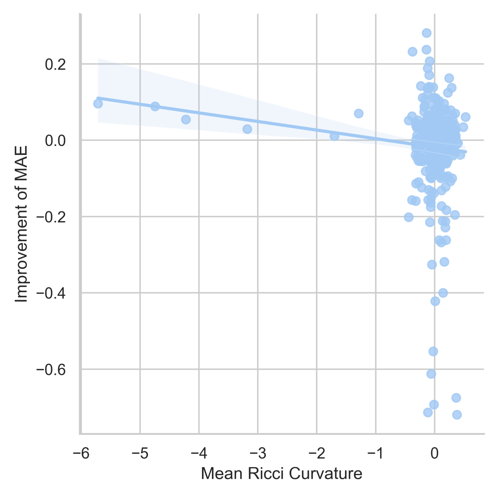
Taking STGCN+ as an example, the relationship between the average curvature of the connected edges of a node κ and the MAE improvement of the model with curvature information is shown in Figure 8. From the figure, it can be found that the κ values in the upper left part of the figure are all negative and have large absolute values, indicating that the corresponding connected edges of these nodes are most likely to be the bottlenecks in the road network. Figure 9 shows two nodes that lie in this category. The pair of nodes are located at intersections, which play an important role in the connectivity of the road network system, and removing the negative curvature edges connected to them is likely to disconnect the road network [27,41]. The addition of the curvature information that represents the bottleneck degree can improve the accuracy of the prediction results of this part of the nodes, and in this part, the larger the absolute value of κ , the more the improvement of MAE. Overall, the curvature graph convolution module can improve the prediction performance of the spatiotemporal graph neural network when evaluated at the scale of the whole road network, and the improvement is especially significant for nodes connected with more bottleneck edges.

4.4.3. Qualitative Visualization Analysis

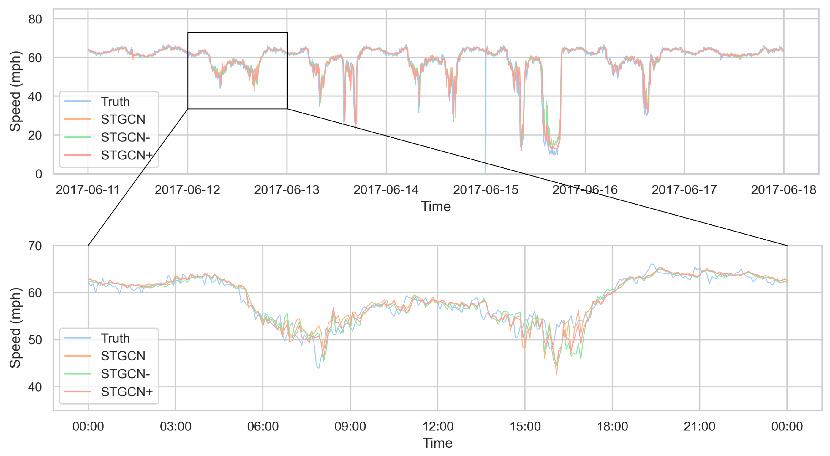
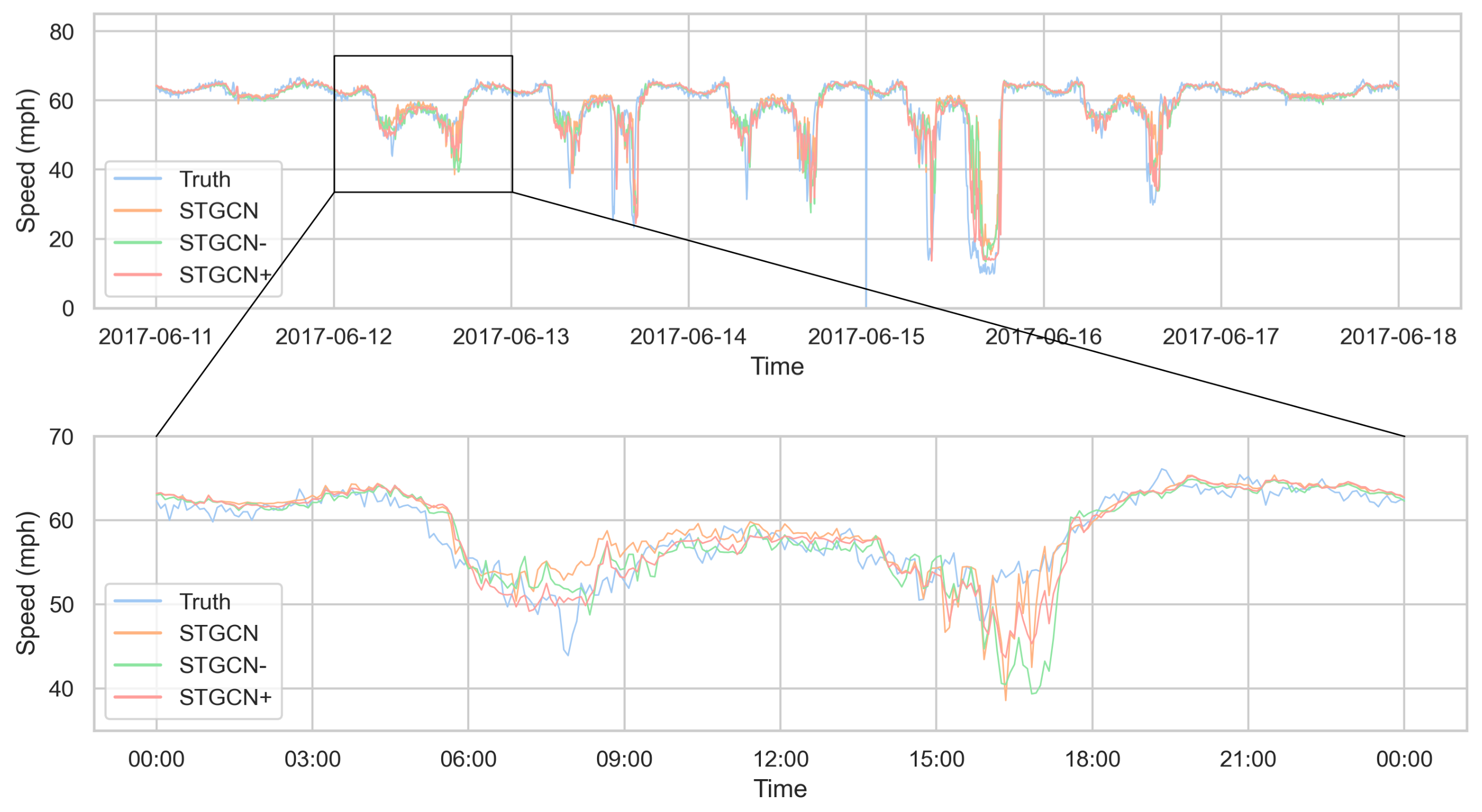
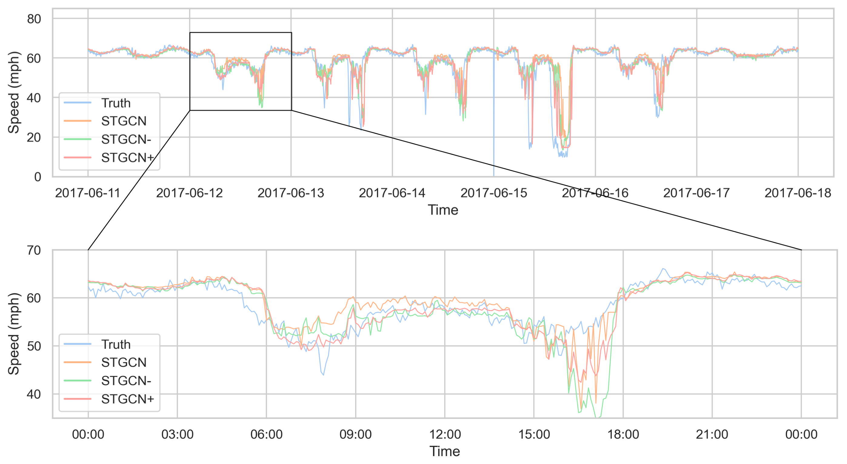
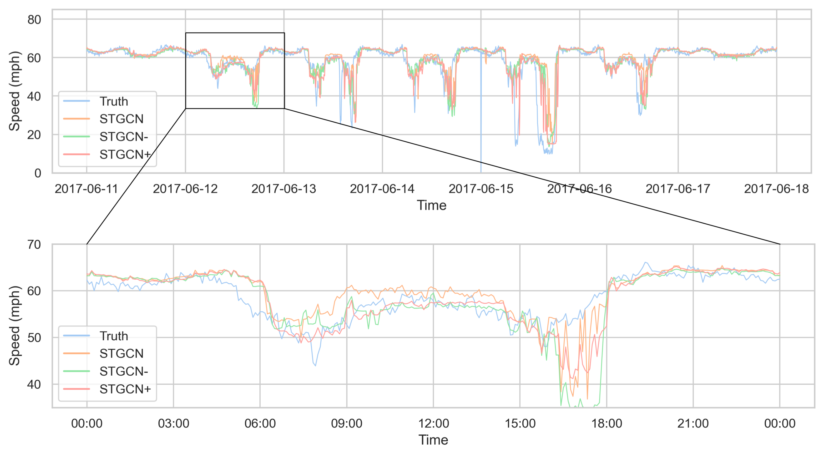
To intuitively compare the prediction performance of each model, the prediction results of STGCN-, STGCN, and STGCN+ with different prediction horizons on the PEMS-BAY dataset are visualized in this paper, as shown in Figure 10, Figure 11, Figure 12 and Figure 13. It can be observed that all three models obtain prediction results that align with the actual trends because the models themselves have a strong ability to learn the temporal dependence. In addition, the prediction performance of the three models gradually deteriorates as the prediction horizon increases, which is limited by the structure of the models themselves.
However, the forecasting results of the three models still show some differences. For example, on the morning of June 12th, the prediction results of STGCN+ fit the ground truth value better, while the prediction results of STGCN gradually deviate with the increase in the prediction horizon. For the more volatile temporal features such as spikes and troughs, such as the trough of the evening peak on the 15th day, the prediction results of STGCN+ are also closer to the ground truth, while the predictions given by STGCN are higher than actual values. Overall, the predictions of STGCN+ are more accurate, which indicates that taking local topological information of the road network into account helps the model to capture spatial dependence better and improve prediction performance.

5. Conclusions and Future Work

Existing methods ignore the effect of the local complex topology of traffic networks on the spatial dependence between nodes. To address the issue, in this paper, we propose a message-passing strategy that comprehensively considers the direct relations between nodes and the relations between neighbors of nodes. For example, nodes in a network form communities, and traffic connections between communities are more dependent on certain paths called bottleneck paths. Specifically, in this paper, we propose a curvature graph convolution module, which is based on the Ollivier–Ricci curvature, to measure the bottleneck degree of road connectivity and apply this information to guide the message-passing process of STGNNs to capture spatial dependence. We compare the performance of STGNNs based on three different graph structures for message passing. Experiments on two real-world traffic speed and flow datasets show that the models based on the curvature graph convolution module perform consistently better than the models based on distance or adjacency graph structures for message passing at 15/30/45 min horizons. As it is possible that the node-to-node and neighborhood-to-neighborhood relationships behind traffic flow data can contribute to the spatial dependence modeling from different perspectives, which can handle complex traffic scenarios potentially, in the future, we will make attempts to incorporate multiple topology properties to exploit further the impact of topological structures of the road network on traffic flow.

Author Contributions

Conceptualization, X.H. and L.Z.; methodology, X.H. and G.Z.; software, G.Z.; validation, X.H.; formal analysis, X.H., Y.W. and Z.C.; investigation, G.Z.; resources, S.H.; data curation, L.Z.; writing—original draft preparation, X.H. and G.Z.; writing—review and editing, R.D., Y.L. and S.H.; visualization, X.H.; supervision, R.D. and S.H.; project administration, S.H. All authors have read and agreed to the published version of the manuscript.

Funding

This work was partly supported by the National Natural Science Foundation of China, Grant/Award Numbers: 42271481; the High-Performance Computing Platform of Central South University and HPC Central of Department of GIS, in providing HPC resources.

Institutional Review Board Statement

Not applicable.

Informed Consent Statement

Not applicable.

Data Availability Statement

Data sharing not applicable.

Acknowledgments

We acknowledge the High-Performance Computing Platform of Central South University and HPC Central of the Department of GIS for providing HPC resources.

Conflicts of Interest

The authors declare no conflict of interest.

Abbreviations

The following abbreviations are used in this manuscript:
STGNNSpatio-temporal Graph Neural Network
GNNGraph Neural Networks
MPNNMessage Passing Neural Networks
CNNConvolutional Neural Networks
RNNRecurrent Neural Networks
GRUGated Recurrent Unit
ARIMAAutoregressive Integrated Moving Average

References

  1. Krizhevsky, A.; Sutskever, I.; Hinton, G.E. Imagenet classification with deep convolutional neural networks. Adv. Neural Inf. Process. Syst. 2012, 25, 84–90. [Google Scholar] [CrossRef]
  2. Bui, K.H.N.; Cho, J.; Yi, H. Spatial-temporal graph neural network for traffic forecasting: An overview and open research issues. Appl. Intell. 2021, 52, 2763–2774. [Google Scholar] [CrossRef]
  3. Gilmer, J.; Schoenholz, S.S.; Riley, P.F.; Vinyals, O.; Dahl, G.E. Neural message passing for quantum chemistry. In Proceedings of the International Conference on Machine Learning, PMLR, Baltimore, MA, USA, 20–23 February 2023; pp. 1263–1272. [Google Scholar]
  4. Guo, K.; Hu, Y.; Qian, Z.; Liu, H.; Zhang, K.; Sun, Y.; Gao, J.; Yin, B. Optimized graph convolution recurrent neural network for traffic prediction. IEEE Trans. Intell. Transp. Syst. 2020, 22, 1138–1149. [Google Scholar] [CrossRef]
  5. Xu, D.; Dai, H.; Wang, Y.; Peng, P.; Xuan, Q.; Guo, H. Road traffic state prediction based on a graph embedding recurrent neural network under the SCATS. Chaos Interdiscip. J. Nonlinear Sci. 2019, 29, 103125. [Google Scholar] [CrossRef] [PubMed]
  6. Wu, T.; Chen, F.; Wan, Y. Graph attention LSTM network: A new model for traffic flow forecasting. In Proceedings of the 2018 5th International Conference on Information Science and Control Engineering (ICISCE), Zhengzhou, China, 20–22 July 2018; pp. 241–245. [Google Scholar]
  7. Li, Y.; Yu, R.; Shahabi, C.; Liu, Y. Diffusion convolutional recurrent neural network: Data-driven traffic forecasting. arXiv 2017, arXiv:1707.01926. [Google Scholar]
  8. Kang, Z.; Xu, H.; Hu, J.; Pei, X. Learning dynamic graph embedding for traffic flow forecasting: A graph self-attentive method. In Proceedings of the 2019 IEEE Intelligent Transportation Systems Conference (ITSC), Auckland, New Zealand, 27–30 October 2019; pp. 2570–2576. [Google Scholar]
  9. Lee, K.; Rhee, W. DDP-GCN: Multi-graph convolutional network for spatiotemporal traffic forecasting. Transp. Res. Part C Emerg. Technol. 2022, 134, 103466. [Google Scholar] [CrossRef]
  10. Ollivier, Y. Ricci curvature of Markov chains on metric spaces. J. Funct. Anal. 2009, 256, 810–864. [Google Scholar] [CrossRef]
  11. LeCun, Y.; Bengio, Y.; Hinton, G. Deep learning. Nature 2015, 521, 436–444. [Google Scholar] [CrossRef]
  12. Oord, A.v.d.; Dieleman, S.; Zen, H.; Simonyan, K.; Vinyals, O.; Graves, A.; Kalchbrenner, N.; Senior, A.; Kavukcuoglu, K. Wavenet: A generative model for raw audio. arXiv 2016, arXiv:1609.03499. [Google Scholar]
  13. Zhang, J.; Zheng, Y.; Qi, D. Deep spatio-temporal residual networks for citywide crowd flows prediction. In Proceedings of the AAAI Conference on Artificial Intelligence, Phoenix, AR, USA, 12–17 February 2016; Volume 31. [Google Scholar]
  14. Ali, A.; Zhu, Y.; Zakarya, M. A data aggregation based approach to exploit dynamic spatio-temporal correlations for citywide crowd flows prediction in fog computing. Multimed. Tools Appl. 2021, 80, 31401–31433. [Google Scholar] [CrossRef]
  15. Kipf, T.N.; Welling, M. Semi-Supervised Classification with Graph Convolutional Networks. In Proceedings of the 5th International Conference on Learning Representations, Toulon, France, 24–26 April 2017. [Google Scholar]
  16. Zhang, M.; Chen, Y. Link prediction based on graph neural networks. Adv. Neural Inf. Process. Syst. 2018, 31, 5171–5181. [Google Scholar]
  17. Li, H.; Cao, J.; Jun, J.; Luo, Q.; He, S.; Wang, X. Augmentation-Free Graph Contrastive Learning of Invariant-Discriminative Representations. IEEE Trans. Neural Networks Learn. Syst. 2023. [Google Scholar] [CrossRef] [PubMed]
  18. Zhao, L.; Song, Y.; Zhang, C.; Liu, Y.; Wang, P.; Lin, T.; Deng, M.; Li, H. T-GCN: A temporal graph convolutional network for traffic prediction. IEEE Trans. Intell. Transp. Syst. 2020, 21, 3848–3858. [Google Scholar] [CrossRef]
  19. Zhu, J.; Han, X.; Deng, H.; Tao, C.; Zhao, L.; Wang, P.; Lin, T.; Li, H. KST-GCN: A knowledge-driven spatial-temporal graph convolutional network for traffic forecasting. IEEE Trans. Intell. Transp. Syst. 2022, 23, 15055–15065. [Google Scholar] [CrossRef]
  20. Ali, A.; Zhu, Y.; Zakarya, M. Exploiting dynamic spatio-temporal graph convolutional neural networks for citywide traffic flows prediction. Neural Netw. 2022, 145, 233–247. [Google Scholar] [CrossRef]
  21. Yu, B.; Yin, H.; Zhu, Z. Spatio-temporal graph convolutional networks: A deep learning framework for traffic forecasting. arXiv 2017, arXiv:1709.04875. [Google Scholar]
  22. Wu, Z.; Pan, S.; Long, G.; Jiang, J.; Zhang, C. Graph wavenet for deep spatial-temporal graph modeling. arXiv 2019, arXiv:1906.00121. [Google Scholar]
  23. Lv, Y.; Duan, Y.; Kang, W.; Li, Z.; Wang, F.Y. Traffic flow prediction with big data: A deep learning approach. IEEE Trans. Intell. Transp. Syst. 2014, 16, 865–873. [Google Scholar] [CrossRef]
  24. Li, M.; Zhu, Z. Spatial-temporal fusion graph neural networks for traffic flow forecasting. In Proceedings of the AAAI Conference on Artificial Intelligence, Virtually, 2–9 February 2021; Volume 35, pp. 4189–4196. [Google Scholar]
  25. He, S.; Shin, K.G. Towards fine-grained flow forecasting: A graph attention approach for bike sharing systems. In Proceedings of the Web Conference 2020, Taipei, Taiwan, 20–24 April 2020; pp. 88–98. [Google Scholar]
  26. Samal, A.; Sreejith, R.; Gu, J.; Liu, S.; Saucan, E.; Jost, J. Comparative analysis of two discretizations of Ricci curvature for complex networks. Sci. Rep. 2018, 8, 8650. [Google Scholar] [CrossRef]
  27. Ni, C.C.; Lin, Y.Y.; Luo, F.; Gao, J. Community detection on networks with Ricci flow. Sci. Rep. 2019, 9, 1–12. [Google Scholar] [CrossRef]
  28. Gao, L.; Liu, X.; Liu, Y.; Wang, P.; Deng, M.; Zhu, Q.; Li, H. Measuring road network topology vulnerability by Ricci curvature. Phys. A Stat. Mech. Its Appl. 2019, 527, 121071. [Google Scholar] [CrossRef]
  29. Wang, Y.; Huang, Z.; Yin, G.; Li, H.; Yang, L.; Su, Y.; Liu, Y.; Shan, X. Applying Ollivier-Ricci curvature to indicate the mismatch of travel demand and supply in urban transit network. Int. J. Appl. Earth Obs. Geoinf. 2022, 106, 102666. [Google Scholar] [CrossRef]
  30. Wang, C.; Jonckheere, E.; Banirazi, R. Wireless network capacity versus Ollivier-Ricci curvature under Heat-Diffusion (HD) protocol. In Proceedings of the 2014 American Control Conference, Portland, OR, USA, 4–6 June 2014; pp. 3536–3541. [Google Scholar]
  31. Forman, R. Bochner’s method for cell complexes and combinatorial Ricci curvature. Discret. Comput. Geom. 2003, 29, 323–374. [Google Scholar] [CrossRef]
  32. Weber, M.; Saucan, E.; Jost, J. Characterizing complex networks with Forman-Ricci curvature and associated geometric flows. J. Complex Netw. 2017, 5, 527–550. [Google Scholar] [CrossRef]
  33. Saucan, E.; Wolansky, G.; Appleboim, E.; Zeevi, Y.Y. Combinatorial ricci curvature and laplacians for image processing. In Proceedings of the 2009 2nd International Congress on Image and Signal Processing, Tianjin, China, 17–19 October 2009; pp. 1–6. [Google Scholar]
  34. Peyré, G.; Cuturi, M. Computational Optimal Transport. Found. Trends Mach. Learn. 2019, 11, 355–607. [Google Scholar] [CrossRef]
  35. Arjovsky, M.; Chintala, S.; Bottou, L. Wasserstein generative adversarial networks. In Proceedings of the International Conference on Machine Learning, PMLR, Singapore, 20–23 February 2023; pp. 214–223. [Google Scholar]
  36. Kusner, M.; Sun, Y.; Kolkin, N.; Weinberger, K. From word embeddings to document distances. In Proceedings of the International Conference on Machine Learning, PMLR, Singapore, 20–23 February 2023; pp. 957–966. [Google Scholar]
  37. Li, H.; Cao, J.; Zhu, J.; Liu, Y.; Zhu, Q.; Wu, G. Curvature graph neural network. Inf. Sci. 2022, 592, 50–66. [Google Scholar] [CrossRef]
  38. Liu, Z.; Zhou, J. Introduction to graph neural networks. Synth. Lect. Artif. Intell. Mach. Learn. 2020, 14, 1–127. [Google Scholar]
  39. Paszke, A.; Gross, S.; Massa, F.; Lerer, A.; Bradbury, J.; Chanan, G.; Killeen, T.; Lin, Z.; Gimelshein, N.; Antiga, L. PyTorch: An imperative style, high-performance deep learning library. Adv. Neural Inf. Process. Syst. 2019, 32, 8026–8037. [Google Scholar]
  40. Wang, J.; Jiang, J.; Jiang, W.; Li, C.; Zhao, W.X. Libcity: An open library for traffic prediction. In Proceedings of the 29th International Conference on Advances in Geographic Information Systems, Beijing, China, 2–5 November 2021; pp. 145–148. [Google Scholar]
  41. Ni, C.C.; Lin, Y.Y.; Gao, J.; Gu, X.D.; Saucan, E. Ricci curvature of the internet topology. In Proceedings of the 2015 IEEE conference on computer communications (INFOCOM), Hong Kong, China, 26 April–1 May 2015; pp. 2758–2766. [Google Scholar]
Figure 1. Road network graph structure of existing traffic forecasting STGNNs for message passing. (a) Adjacency graph: node x1, x2, and x3 have the same impact on the traffic flow of x. (b) Spatial distance graph: closer nodes have a stronger impact on the traffic state of the target node.
Symmetry 15 00995 g001
Figure 2. The bottleneck edge in road network.
Symmetry 15 00995 g002
Figure 3. An illustration of message passing in graph neural networks.
Symmetry 15 00995 g003
Figure 4. Illustration of the Ollivier–Ricci curvature of edges on a graph. The weights of edges in (ac) are 1. (a) Graph with tree structure, edges connecting each subtree (marked in red) have negative curvature; (b) infinite uniform grid graph, all edges have zero curvature; (c) complete graph, all edges have positive curvature.
Symmetry 15 00995 g004
Figure 5. The distribution of traffic speed in the PEMS-BAY dataset.
Symmetry 15 00995 g005
Figure 6. The distribution of traffic speed in the PEMSD7 dataset.
Symmetry 15 00995 g006
Figure 7. Different graph structures of the traffic network. (a) Spatial distance graph. (b) Adjacency graph. (c) Local topological structure enhanced graph.
Symmetry 15 00995 g007
Figure 8. MAE improvement of prediction results for each node of STGCN+ compared to STGCN on the PEMS-BAY dataset.
Symmetry 15 00995 g008
Figure 9. Examples of nodes connected to edges with high negative curvature.
Symmetry 15 00995 g009
Figure 10. Visualization of 15 min-ahead predictions of different models.
Symmetry 15 00995 g010
Figure 11. Visualization of 30 min-ahead predictions of different models.
Symmetry 15 00995 g011
Figure 12. Visualization of 45 min-ahead predictions of different models.
Symmetry 15 00995 g012
Figure 13. Visualization of 60 min-ahead prediction of different models.
Symmetry 15 00995 g013
Table 1. Basic information of two real-world traffic speed and flow datasets.
DatasetNumber of NodesSampling IntervalTime SpanFeature to be Predicted
PEMS-BAY3255 min1 January 2017–30 June 2017Speed
PEMSD78835 min1 July 2016–31 August 2016Flow
Table 2. Comparison setup.
ModelGuidelines for
Message Propagation
Spatial DependencePerspective on Measuring
Relations
BackboneSpatial distance graphSpatial distancenode-to-node
Backbone+Edge bottleneck factor r i j Local topological structureNeighborhood-to-neighborhood
Backbone-Adjacency graphAdjacencynode-to-node
Table 3. Performance of STGNNs based on different message passing strategies on PEMS-BAY.
ModelPEMS_BAY(15/30/45/60 min)
MAEMAPE(%)RMSE
STGCN-1.426/1.904/2.233/2.4913.15/4.63/5.58/6.243.002/4.325/5.122/5.669
STGCN1.423/1.908/2.241/2.5013.13/4.49/5.37/6.002.991/4.284/5.051/5.607
STGCN+1.400/1.878/2.223/2.5162.98/4.34/5.27/6.012.907/4.176/4.983/5.608
TGCN-1.714/2.112/2.381/2.6163.62/4.71/5.41/6.003.228/4.110/4.596/4.990
TGCN2.302/2.659/2.953/3.2064.99/6.03/6.85/7.584.222/5.048/5.614/6.083
TGCN+1.613/2.109/2.464/2.7743.37/4.69/5.68/6.543.147/4.254/4.955/5.494
Table 4. Performance of STGNNs based on different message passing strategies on PEMSD7.
ModelPEMSD7(15/30/45/60 min)
MAEMAPE(%)RMSE
STGCN-21.782/26.689/30.704/36.6619.59/11.96/14.61/17.1033.474/39.730/46.166/52.936
STGCN21.409/25.053/28.437/31.6089.28/10.87/12.41/13.8033.423/38.328/42.671/46.803
STGCN+20.657/24.205/27.600/30.6768.91/10.58/12.32/13.8332.354/37.052/41.413/45.529
TGCN-43.877/46.337/50.332/55.39325.54/26.52/28.67/32.0760.802/64.241/69.519/76.424
TGCN37.439/40.000/43.732/49.14722.89/24,45/27.02/31.2652.751/56.269/61.202/68.157
TGCN+25.883/29.743/34.012/38.83813.01/14.79/17.10/19.8638.186/43.477/48.979/55.259
Disclaimer/Publisher’s Note: The statements, opinions and data contained in all publications are solely those of the individual author(s) and contributor(s) and not of MDPI and/or the editor(s). MDPI and/or the editor(s) disclaim responsibility for any injury to people or property resulting from any ideas, methods, instructions or products referred to in the content.