Communication

Symmetry in Regression Analysis: Perpendicular Offsets—The Case of a Photovoltaic Cell †

by
Lorentz Jäntschi
1,2
1
Chemical Doctoral School, Babes-Bolyai University, 400028 Cluj-Napoca, Romania
2
Department of Physics and Chemistry, Technical University of Cluj-Napoca, 400641 Cluj-Napoca, Romania
This paper is an extended version of our paper which will be published in the 4th International Conference on Symmetry, Barcelona, Spain, 21–23 June 2023.
Symmetry 2023, 15(4), 948; https://doi.org/10.3390/sym15040948
Submission received: 26 March 2023 / Revised: 9 April 2023 / Accepted: 19 April 2023 / Published: 21 April 2023
(This article belongs to the Section Physics)

Abstract

:
It is known that, for paired measurements subjected to experimental error, better suited linear regression is obtained by using perpendicular offsets. Even so, the great majority of statistical software still uses classical vertical offsets for reasons of convenience. The same convenience leads to the preference of the least squares method in the favor of maximum-likelihood estimation. The treatise for perpendicular offsets for simple linear regression is slightly trickier than the corresponding one for vertical offsets. However, there is no general treatise for perpendicular offsets for nonlinear cases to date. In this work, a typical case of nonlinear dependence—potential versus intensity of current produced by a photovoltaic cell—is subjected to study. A series of paired potential/current data was collected from a commercial photovoltaic device and served for introducing the perpendicular offsets approach in the case of a nonlinear regression. Photovoltaic cell parameters—internal resistance, short-circuit current intensity, potential of open-circuit, and the maximum power point—have been determined by using the perpendicular offsets approach. Several issues were addressed in this work, such as exploring the intrinsic symmetry in the treatment of current versus potential diagrams, the suitability of perpendicular offsets in obtaining of the regression coefficients, and the implementation of nonlinear regression models with perpendicular offsets. Even if both the treatises of perpendicular offsets and nonlinear regression are known for some time now, there is no report in the literature of using both. Furthermore, since both potential and current measurements are affected by errors, it is more natural to use the proposed approach of perpendicular offsets.

1. Introduction

1.1. History

Electron transfer is the basic principle of batteries, solar cells, and, in the case of living organisms, chlorophylls. It appears that plants were the first here as well through the discovery of photosynthesis [1]. Based on these first studies of electricity, Woodward [2] completed a long journey of clarifying chlorophyll’s role in the conversion of light into chemical energy.
In the meanwhile, Luigi Galvani, who was studying biological tissue [3], was among the first to provide evidence for the movement of the electrical charge. Going further with the Voltaic pile, Alessandro Giuseppe Antonio Anastasio Volta was the first to develop, with a simple construction (Figure 1 adapted from [4]), a power source that could continuously provide an electric current to a circuit.
Solar cells produce electricity from sunlight, and the first study regarding this was conducted in 1839 [5], while the first device was patented at the beginning of the 20th century [6]. A photovoltaic cell (PV cell) is a specialized semiconductor diode that converts visible light (VIS) or infrared (IR) or ultraviolet (UV) radiation into current. In a commercial technology, silicon is mixed with copper and hydrochloric acid to produce trichlorosilane gas, which is then reduced with hydrogen to make silane gas. Silane gas is heated in molten silicon, resulting in silicon crystals that can be reformed and used for photovoltaic cells and microchips.

1.2. Today

It should be noted that the modern solar cells may have over 10% efficiency, which can be further improved up to nearly 20% [7], and they surpass the efficiency of the chlorophylls, averaged at 1% [8], with a peak efficiency of about 3% and a theoretical efficiency of 9% [9]. A record for solar cell efficiency, namely 47.1%, was recently achieved by using multi-junction concentrator [10]. However, there is a long way to go in order transfer this peak performance into mass production. Recent developments in organic photovoltaic cells have made significant advancements in power conversion efficiency from 3% to over 15% since their introduction in the 1980s [11], while porphyrin-based organic/inorganic hybrid solar cells were reported working at peak efficiency of 19% in [12]. Additionally, it should be noted that there is a higher expectancy in terms of efficiency from PV is expected even more since their performance may be increased by continuous alignment [13,14].
In many instances, regression analysis implies a linear model (see [15] for a step-by-step coverage of linear models from model specification to capacity of prediction and [16] for an extent of them to include non-Gaussian errors). Additionally, in some instances, linearization is also a good alternative (see [17] for a general treatise of functional transformations, ref. [18] for applicability domain of the linearization, and [19] for a case of automated linearization).
However, current-voltage dependence of a photovoltaic (PV) is known to be nonlinear [20], and a series of alternatives are considered (symbolic regression combined with multilayer perceptron in [21], nonlinear autoregressive with exogenous input neural network in [22], artificial population-based metaheuristic algorithm of differential evolution in [23], slime mold optimization in [24], barnacle mating optimization algorithm in [25]).
In order to obtain a higher accuracy, the models for the power sources have recently become more and more elaborated [26]. The recent energy crisis has proven that more attention should be directed towards alternative and renewable sources of energy, and among those, PVs attracted a special interest. Thus, modeling of solar generating systems for patterning the performance under various conditions of solar irradiance, temperature, and loading is investigated in [25] using the barnacle mating optimization algorithm, in [27] with the hunter–prey optimizer, in [28] with the whale optimizer, and in [29] with principal component analysis, while some low computational intensity models are proposed in [26].

1.3. Aim

In this study, the parameters of a commercial solar cell have been investigated. The study provides grounds for a theoretical discussion regarding the use of perpendicular offsets into the analysis of nonlinear regression.

2. Materials and Methods

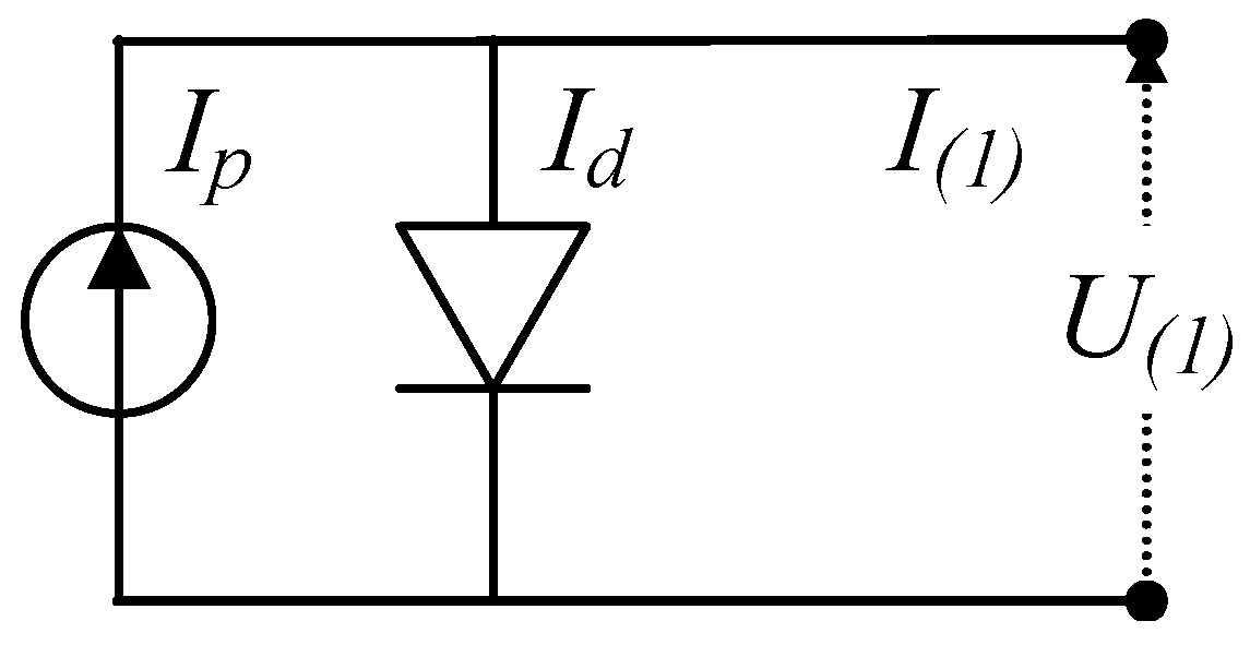
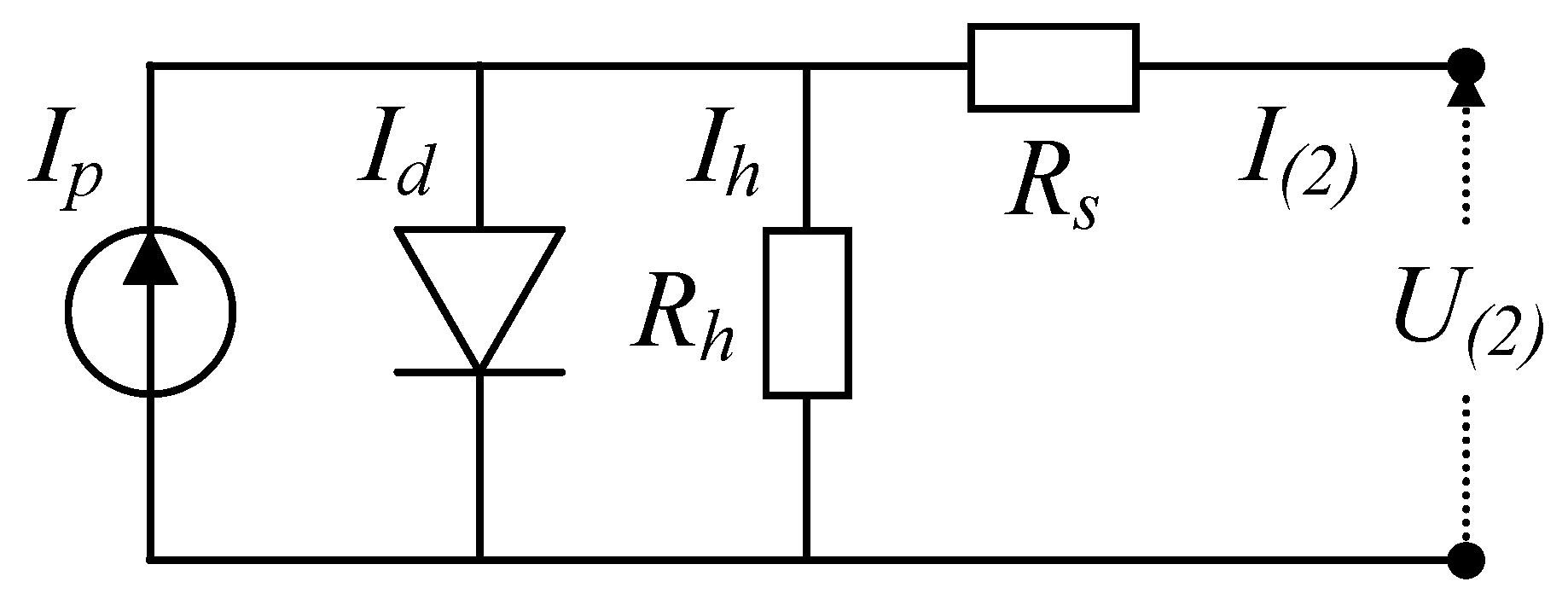
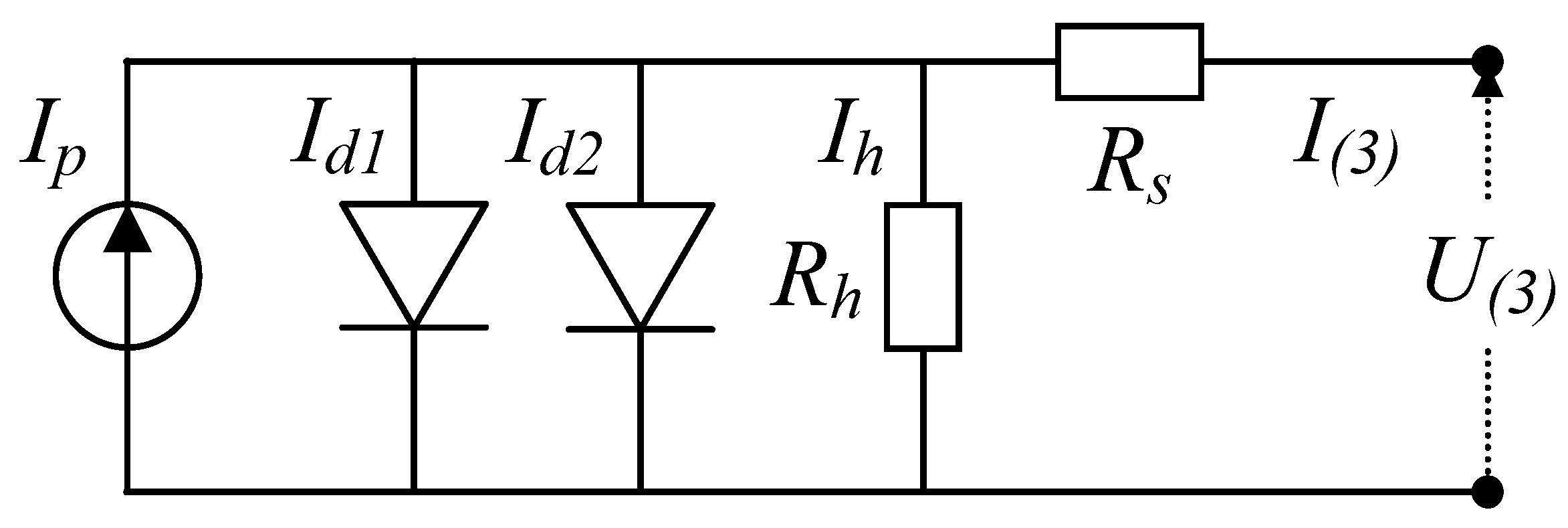
2.1. Single-Diode, Double-Diode, and PV Generator Models

A PV cell is given in terms of output current (I) and voltage (U). Several models have been developed to describe the I U characteristic of solar cells.
The simplest model of a PV (Figure 2) is made from a current source ( I p ) in parallel with a diode ( I d ).
If V T is the thermal voltage, and  η is the diffusion and recombination diode ideality factor, then (by using I p = I d + I relation) the simplest model (Figure 2) can be formulated as follows:
I ( 1 ) = I p I 0 ( exp ( U ( 1 ) η V T 1 ) )
where I 0 is the diode reverse saturation current.
The initial formula of a diode direct current was derived without the ideality factor [30] and added later to correct for non-ideal behavior (adjusted empirically to make the equation fit the data [31]; for the case reported in [31], η was found about 1.03. An  η 1 is assumed to be representative of a second-order (bimolecular) radiative recombination of free charges, whereas η 2 is attributed to a first-order (monomolecular) nonradiative recombination process [32]. Furthermore, some authors notice variations in η values among diodes from different producers at the same current intensities but also for same diodes at different current intensities [33].
In practice, no solar cell is ideal, so two passive components, a shunt resistance ( R h , emulating tiny electric shorts through the PN junction of the PV cell) and a series resistance ( R s , emulating the internal losses of the PV cell) are added to the model in order to compensate for the nonideality (Figure 3).
The relation between output current (I) and voltage (U) is updated from Equation (1) for Figure 2 to Equation (2) for Figure 3 by considering the passive components added ( U ( 2 ) = U ( 1 ) I ( 2 ) R s , I ( 2 ) = I ( 1 ) I h , U ( 1 ) = I h R h = U ( 2 ) + I ( 2 ) R s ):
I ( 2 ) = I p I 0 ( exp ( U ( 2 ) + I ( 2 ) R s η V T 1 ) ) U ( 2 ) + I ( 2 ) R s R h
In the double-diode model, two parallel connected diodes are used instead of one, resulting in a system like the one in Figure 4.
Again, the relation between output current (I) and voltage (U) is updated, now from Equation (2) for Figure 3 to Equation (3) for Figure 4, and this is accomplished by considering the active components added (now I ( 3 ) = I d 1 + I d 2 + I h + I ( 3 ) instead of I p = I d 1 + I h + I ( 2 ) , or  I ( 3 ) = I ( 2 ) I d 2 , I h R h = U ( 3 ) + I ( 3 ) R s ):
I ( 3 ) = I p I 01 ( exp ( U ( 3 ) + I ( 3 ) R s η 1 V T 1 ) ) I 02 ( exp ( U ( 3 ) + I ( 3 ) R s η 2 V T 1 ) ) U ( 3 ) + I ( 3 ) R s R h
where I 01 and I 02 are the reverse saturation currents and  η 1 and η 2 , respectively, the ideality factors.
One can easily realize that the model from Equation (3) becomes more and more complex by adding more active components in it.
A PV generator is a system which usually may be a grid of N s series-connected by N p parallel-connected PV cells, and in that instance, considering those PV cells are undistinguishable, a formula for the output parameters of the PV system can be expressed by updating Equation (2) again [24]:
I P V = N p I p N p I 0 ( exp ( U P V / N s + I P V R s / N p η V T 1 ) ) U P V N p / N s + I P V R s R h
Important parameters of a PV include open-circuit voltage ( V oc ), short-circuit intensity ( I sc ), and its internal resistance ( r i ). Additionally, one point on the I U curve is of interest, the point in which I · U obtains a maximum, which is the maximum power point ( P = I · U , P m a x . P = P xp , P xp = I xp · U xp , where I xp is the current intensity and U xp is the electric potential (voltage) at maximum power, P xp ).

2.2. Lambert Function

The Lambert W function [34], namely the function W from Equation (5), is a useful tool for solving equations involving exponentials [35] and may serve to express a pseudo-analytical form of the solution for Equation (2).
z = W ( z ) exp ( W ( z ) )
Thus, if  I = I ( U ) is to be extracted from Equation (2), then
I = ( I p + I 0 ) R h U R s + R h η V T R s W I 0 R s R h η V T ( R s + R h ) exp ( U + ( I p + I 0 ) R s ) R h η V T ( R s + R h )
and if U = U ( I ) is to be extracted from Equation (2), then
U = ( I p + I 0 ) R h I ( R s + R h ) η V T W I 0 R h η V T exp I p + I 0 I η V T / R h
One will want to bypass the Lambert function in order to express an approximate analytical expression for I = I ( U ) and/or U = U ( I ) . In this case, it should be known that power ( x α ) and exponential ( e x ) functions have a similar shape. Even more so, for  α > e , there always exists an (open) interval in which x α > e x , while outside of this interval x α e x .    

2.3. Explicit Equations
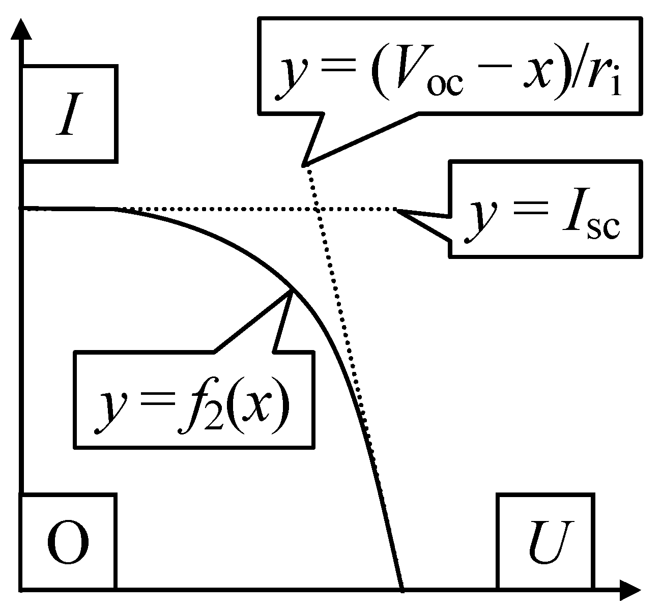
One should notice that, aside from Equation (1), there is no explicit equation describing the I U characteristic. As opposed to analytically solving the equations such as Equation (2) or Equation (3) with Lambert function is by operating on approximate explicit (analytic) function. Here some proposed models are given.
Kalmarkar [36,37] proposed
I I sc = 1 ( 1 c 1 ) U V oc c 1 ( U V oc ) c 2
where c 1 = c 1 ( I xp , U xp , I sc , V oc , c 2 ) and c 2 = c 2 ( I xp , U xp , I sc , V oc ) are the coefficients to be determined.
Das [38,39] proposed
I I sc = 1 ( U V oc ) c 2 1 + c 1 ( U V oc )
where c 1 = c 1 ( I xp , U xp , I sc , V oc , c 2 ) and c 2 = c 2 ( I xp , U xp , I sc , V oc ) are the coefficients to be determined.
Pindado and Cubas [40,41] proposed:
I = I sc ( 1 ( 1 I xp I sc ) ( U U xp ) c 1 ) if U U xp I xp U U x p ( 1 ( U U xp V oc U xp ) c 2 ) otherwise
where c 1 = c 1 ( I xp , U xp , I sc ) and c 2 = c 2 ( I xp , U xp , I sc , V oc ) are the coefficients to be determined.
One should notice that in each of the above given instances four parameters need to be determined ( I xp , U xp , I sc , and  V oc ).
Another remark to be made is on the type of the analytic function. Thus, Equation (8) defines a linear (additive) combination of linear and power functions, Equation (9) defines a rational function, while Equation (10) is a piecewise of power and of linear and power functions.    

2.4. Limit Cases

In a plot of potential versus current ( y = f 1 ( x ) in Figure 5), it is expected to observe a linear oblique tendency for small currents ( y = V oc x · r i line in Figure 5) and a linear vertical tendency for high currents ( x = I sc line in Figure 5).
The plot of current versus potential (Figure 6) is to be obtained from the plot of potential versus current (Figure 5) by two symmetry operations: a rotation with π / 2 and a reflection (D4 symmetry operation).
In a plot of current versus potential ( y = f 2 ( x ) in Figure 6), it is expected to observe the linear oblique tendency for high voltages ( y = ( V oc x ) / r i line in Figure 6) and a linear horizontal tendency for low voltages ( y = I sc line in Figure 6).
One should also notice that the f 1 and f 2 functions are inverse ( f 2 ( f 1 ( x ) = x ). Due to the two linear trends (lines depicted as y = V oc x · r i and x = I sc in Figure 5 and y = ( V oc x ) / r i and y = I sc in Figure 6), some authors translate the dependence into a bilinear one [42].    

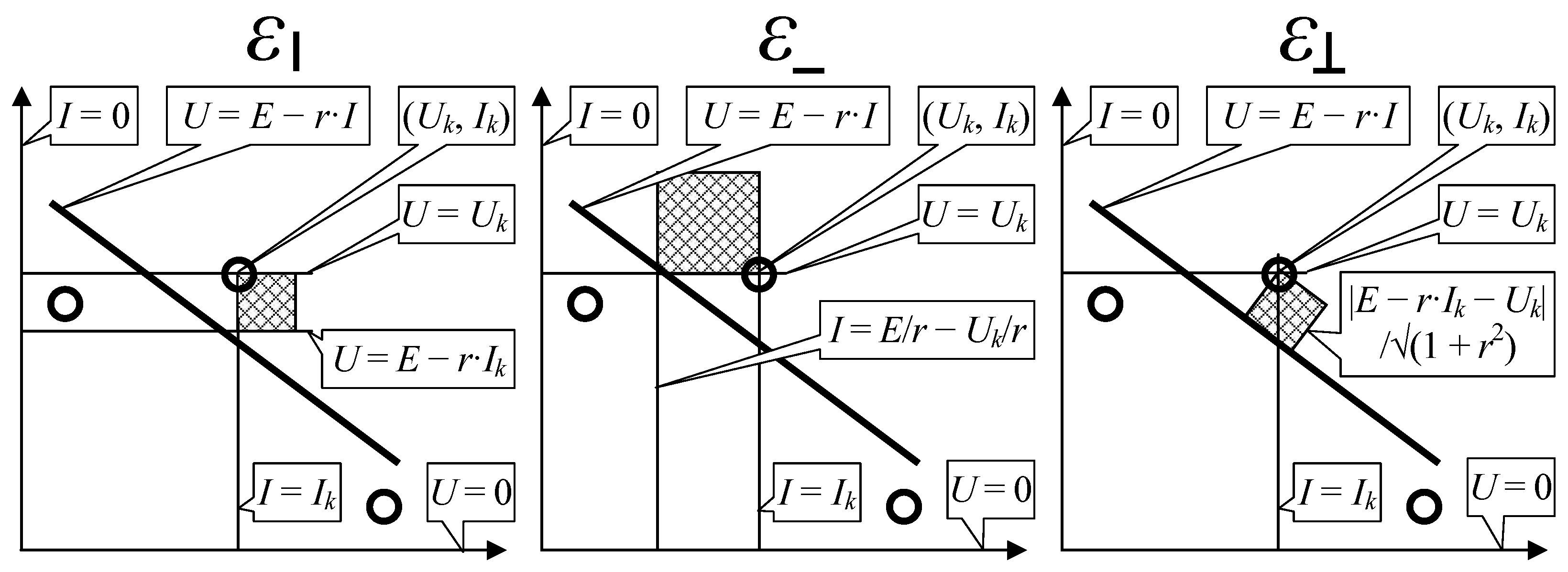
2.5. Minimizing Unexplained Variance (Errors)

A typical regression method minimizes the sums of squares (Figure 7).
Classical vertical offsets minimize the sums of squares formed with vertical sides from each observation point, k = 1 , 2 , . . . , m (with m the number of experimental paired observations) to the model line ( y = f 1 ( x ) in Figure 5 and y = f 2 ( x ) in Figure 6). One should notice that constructing vertical offsets for potential vs. current (Figure 5) is improper, a paired observation having a very low probability to actually meet the model y = f 1 ( x ) in real frame near the short-circuit intensity ( U , I > 0 ).
Horizontal offsets may be constructed as well (Figure 7). Horizontal offsets minimize the sums of squares formed with horizontal sides from each observation point, k = 1 , 2 , . . . , m (with m the number of experimental paired observations) to the model line ( y = f 1 ( x ) in Figure 5 and y = f 2 ( x ) in Figure 6). One should notice that constructing horizontal offsets for current vs. potential (Figure 6) is improper, a paired observation having very low probability to actually meet the model y = f 2 ( x ) in a real frame near the zero circuit voltage ( U , I > 0 ).
Perpendicular offsets are another alternative (Figure 7). Perpendicular offsets minimize the sums of squares formed with sides constructed perpendicular from each observation point, k = 1 , 2 , . . . , m (with m the number of experimental paired observations) to the model line ( y = f 1 ( x ) in Figure 5 and y = f 2 ( x ) in Figure 6). One should notice that constructing perpendicular offsets is suitable in both instances, potential vs. current (Figure 5) and current vs. potential (Figure 6), as the side of the square minimizes the expectance of an experimental error in all regions (since in a right triangle the height of the right angle is always less than the two sides).

2.6. Occam’s Razor: Two Simple Models

Parsimony law (pluralitas non est ponenda sine necessitate in Latin, plurality should not be posited without necessity in English, known as Occam’s or Ockham’s razor) dictates that one should give precedence to simplicity: of two (or more) competing theories, the simpler explanation of an entity is to be preferred.
Two functions are taken as models here, so as to approximate the non-linear behavior of a PV: a rational function ( f 1 ( x ) from Equation (11), depicted in Figure 8) and a power function ( f 2 ( x ) from Equation (11), depicted in Figure 9):
f 1 ( x ) = a 1 + a 2 x + a 3 x 2 a 4 + x
f 2 ( x ) = b 1 exp ( b 2 + b 3 ln ( x ) )
The similarity between Figure 5 and Figure 8 can be noticed, so the initial (suboptimal) values of the coefficients may be estimated from U = U ( I ) measured data.
The same similarity is seen between Figure 6 and Figure 9, so the initial (suboptimal) values of the coefficients may be again estimated from I = I ( U ) measured data.
Upon having a model for the U = U ( I ) dependence (such as the model in Equation (11)), the open-circuit voltage ( U oc ) is the one at which the circuit is passed by a hypothetical null current ( x = 0 ), and the short-circuit intensity is the one in which the circuit is at null voltage ( f 1 ( x ) = 0 ), so I sc and U oc are given by Equation (13).
If U ( I ) = a 1 + a 2 I + a 3 I 2 a 4 + I U oc = a 1 / a 4 , I sc = a 2 ± a 2 2 4 a 1 a 3 2 a 3
Upon having a model for I = I ( U ) dependence (such as the model in Equation (12)), the open-circuit voltage ( U oc ) is the one at which the circuit is passed by a hypothetical null current ( f 2 ( x ) = 0 ), and the short-circuit intensity is the one in which the circuit is at null voltage ( x = 0 ), so I sc and U oc are given by Equation (14).
If I ( U ) = b 1 exp ( b 2 + b 3 ln ( U ) ) U oc = exp ( ( ln ( b 1 ) b 2 ) / b 3 ) , I sc = b 1
In any instance, the maximum power point is the one in which the U · I product ( x · f ( x ) ) reaches a maximum, so U · I + U · I = 0 ( f ( x ) + x · f ( x ) = 0 ) and
If U ( I ) = a 1 + a 2 I + a 3 I 2 a 4 + I I xp = i 1 3 + i 2 3 , U xp = U ( I xp )
If I ( U ) = b 1 exp ( b 2 + b 3 ln ( U ) ) U xp = b 1 ( 1 + b 3 ) exp ( b 2 ) 1 / b 3
where U xp , I xp , and P xp = U xp · I xp are the values of potential ( U xp ), intensity ( I xp ), and power ( P xp ) at maximum power point, and  i 1 and i 2 from Equation (15) are given by:
i 1 , 2 = q 1 ± q 1 + p 1 3 , p 1 = ( a 2 3 a 3 a 4 ) 2 72 a 3 3 , q 1 = a 2 3 9 a 2 2 a 3 a 4 + 27 a 3 2 a 4 2 ( a 3 a 4 a 2 ) + 54 a 1 a 3 2 a 4 216 a 3 3
The maximum power point is of real interest in solving optimal power flow problems [43,44].

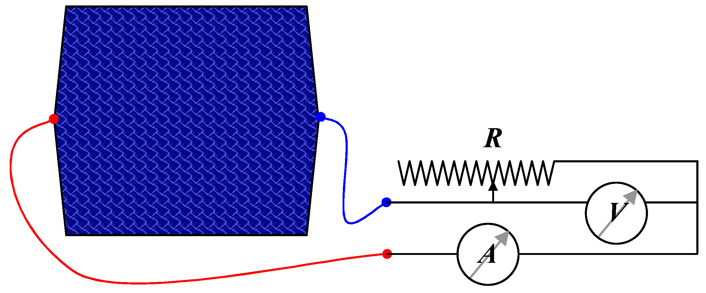
2.7. The Experiment and Data Treatment

The measurements were made in the presence of indoor light by using a simple circuit (Figure 10).
Let us consider ( U k , I k ) for k = 1 , 2 , . . . , m the set of m paired measurements. Since the order in the pair is relevant, the values shall be substituted with variables ( x k , y k ) for k = 1 , 2 , . . . , m . The perpendicular offsets from the observed point ( x k , y k ) to the model function y = f ( x ) can be calculated (see the construction from Figure 11).
If y = f ( x ) then its tangents are y = f ( x 0 ) + f ( x 0 ) · ( x x 0 ) , where x 0 is the ordinate position, ( y = f ( x 0 ) + f ( x 0 ) · ( x x 0 ) is the equation of the tangent to y = f ( x ) in x = x 0 ), where f ( x ) is the function derivative ( f ( x ) = d f ( x ) / d x ). The normal to the y = f ( x ) curve is y = f ( x 0 ) ( x x 0 ) / f ( x 0 ) . If  x = x 0 , then the point on the curve is ( x 0 , f ( x 0 ) ) and the distance (d) from it to an arbitrary observed pair ( x k , y k ) , positioned on the normal to the curve ( y k = f ( x 0 ) ( x k x 0 ) / f ( x 0 ) ), is given by Equation (18):
d ( ( x 0 , f ( x 0 ) ) , ( x k , y k ) ) = ( x 0 x k ) 2 + ( f ( x 0 ) y k ) 2
while the point itself (more exactly, its abscisa, x 0 ) is to be calculated from another nonlinear equation, Equation (19):
x 0 s . th . y k = f ( x 0 ) ( x k x 0 ) / f ( x 0 )
Even if the situation looks discouraging at first glance, it is actually not so complicated since x 0 belonging to the normal to the curve will minimize the distance (and its square) from Equation (18), so the problem is equivalent to Equation (20):
x 0 s . th . y k = ( x 0 x k ) + ( f ( x 0 ) y k ) 2 is minimum

3. Results and Discussion

The results of the measurements are given in Table 1.

3.1. Implementation of the Proposed Solution

Identifying the point of intersection between the curve y = f ( x ) and the perpendicular from the observed point ( x k , y k ) should not possess a challenge to the improved Levenberg–Marquardt optimizer (for the Levenberg method see [45], for the Marquardt implementation see [46] and for its improvement see [47]), since Equation (20) is used, and especially since x · f ( x ) is unimodal (in the present experiment, common sense dictates that there is only one point with maximum power). Its AlgLib [48] implementation has been used under Free Pascal environment [49]. The Levenberg–Marquardt method is among the most applied algorithms due to its flexibility and fast convergence [50]. Some of its limitations are reported as well, such as the number of parameters and the estimation errors of the initial parameters being the main factors limiting the retrieval accuracy of the algorithm [51].
For ( c 1 , , c n ) , a given set of coefficients (a function such as the one from Equation (11) or Equation (12), or any other mathematical function approximating the Equation (2)), the expression of the function becomes completely known and Equation (19) or Equation (20) provides a way towards perpendicular offsets from each observed point. In this context, another optimization can be conducted, namely to minimize the Equation (21) sums, where z k are ordinates of points provided by Equation (20), and  f ( z k ; c 1 , , c n ) is the function f ( x ) evaluated in x z k using c 1 , , c n as given coefficients:
c 1 , , c n s . th . k = 0 m ( z k x k ) 2 + k = 0 m ( f ( z k ; c 1 , , c n ) y k ) 2 is minimum
The algorithm providing perpendicular offsets is given as Algorithm 1 below.   
Algorithm 1: Providing perpendicular offsets.
//Uses Minimize function solving an optimization problem (Equation (21))
//f is a function variable implementing a function like Equation (11) or Equation (12)
//Implement pf function below
Input:
   m //sample size
    ( X , Y ) //sample data ( X = { x 1 , , x m } , Y = { y 1 , , y m } )
   n //number of coefficients
   C //initial guess for coefficients ( C = { c 1 , , c n } )
   f //function evaluating the model with given coefficients ( f = f ( x ; C ) )
   k //data pair index from which to construct the perpendicular offsets
Function  PF ( m , X , Y , n , C , f , k )
    z X [ k ] ; t MINIMIZE ( ( z X [ k ] ) 2 + ( f ( z ; C ) Y [ k ] ) 2 , z )
   Return  ( t X [ k ] ) 2 + ( f ( t ; C ) Y [ k ] ) 2
EndFunction
r p f ( m , X , Y , n , C , f , k )
Output:
   r //the squared perpendicular offset from k to f
In Algorithm 1, the improved Levenberg–Marquardt optimizer was used for the minimize function, as mentioned above, but the implemented solution can be more general, and any other optimizer can be used. One might prefer, for instance, other libraries for optimization, such as Mathcad [52], Mathematica [53], or Matlab [54].
The algorithm constructing the sum of perpendicular offsets is given as Algorithm 2.
Algorithm 2: Sum of perpendicular offsets.
//Uses function pf defined in Algorithm 1 & implement function sp below
Input:
   m //sample size
    ( X , Y ) //sample data ( X = { x 1 , , x m } , Y = { y 1 , , y m } )
   n //number of coefficients
   C //initial guess for coefficients ( C = { c 1 , , c n } )
   f //function evaluating the model with given coefficients ( f = f ( x ; C ) )
Function  SP ( m , X , Y , n , C , f )
    r 0 ; For ( k 1 , , m ) r r + p f ( m , X , Y , n , C , f , k )  EndFor
   Return r
EndFunction
s s p ( m , X , Y , n , C , f )
Output:
   s //sum of the squared perpendicular offsets
Algorithm 2 constructs the objective function for the second optimization phase by calculating the sums provided as Equation (21), which are of the squares of the perpendicular offsets.
The algorithm providing a solution to the nonlinear regression problem is given as Algorithm 3.
Algorithm 3: Nonlinear regression with perpendicular offsets.
//Uses Minimize function solving an optimization problem (Equation (21))
//Uses InitialEstimate function providing an initial guess
//Uses function sp defined in Algorithm 2
Input:
   m //sample size
    ( X , Y ) //sample data ( X = { x 1 , , x m } , Y = { y 1 , , y m } )
   n //number of coefficients
   C //initial guess for coefficients ( C = { c 1 , , c n } )
   f //function evaluating the model with given coefficients ( f = f ( x ; C ) )
C INITALESTIMATE ( m , X , Y , n , f ) //or any other good guess initialization
D MINIMIZE ( SP ( m , X , Y , n , C , f ) , C )
Output:
   D //coefficients minimizing the sum of the perpendicular offsets
In Algorithm 3, the InitialEstimate function is merely used to provide an adequate initial guess, it may use maximum likelihood (like in the instance reported in [55]), but any other strategy providing an adequate initial guess can be used instead (such as classical least squares in [56]). In some instances, better guesses may be derived using transformed data (such as in [57]).

3.2. The Numerical Results

In this situation, rough approximations are used to provide the initial estimates. Table 2 provides the values of these estimates (and where all coefficients were identified as being highly statistically significant).
The optimization was run in both instances for a considerable amount of iterations (Figure 12 and Figure 13). In each iteration, about 290 steps of optimization are required to have all offsets perpendicular, and about 196 steps of optimization are required to have all offsets perpendicular by starting from vertical ones ( z X [ k ] in Algorithm 1).
Because of the double-embedded optimization (made by Algorithm 1, embedded into function sp in Algorithm 2, and subject to another optimization in Algorithm 3), the convergence is slow—millions of iterations are required to reach the optimum point. To be precise, 2,482,076,218 evaluations of f 1 function were used to obtain perpendicular offsets for it in 8,581,798 evaluations of sp function from Algorithm 2, and 1,072,445,080 evaluations of f 2 function were used to obtain perpendicular offsets for it in 5,477,230 evaluations of sp function from Algorithm 2. In all instances, the convergence becomes smooth almost instantly (see the jump at the beginning of the iterations in Figure 12 and Figure 13).
Table 3 contains the results of the optimization. One should note that, even if the initial feed data were distinct ( X I , Y U for f 1 and X U , Y I for f 2 ), the meaning of the residual sum of squares ( R S S ) is the same (via Equation (20)), which allows comparison of the models.
Both models have asymptotic tendencies (to a vertical line in x = a 4 and to a oblique line in x = 0 for f 1 ; to a horizontal line in x = 0 for f 2 ). Model f 1 defined by Equation (11) is a rational function, which is known to fit well in nonlinear problems, while model f 2 , defined by Equation (12), is a transformed power function ( f 2 ( x ) = b 1 e x p ( b 2 ) x b 3 ). The analysis of the residual ( R S S in Table 3) reveals that its value is smaller for the estimation using f 2 function than for the estimation using f 1 function, even if f 2 uses fewer parameterization coefficients. This result is difficult to attribute to chance. Thus, f 2 can be considered a good prediction model for I = I ( U ) dependency of the PV system.
One should notice that f 2 uses only three unknown parameters (from which one of them, namely b 1 , has a direct physical interpretation, b 1 = I sc ), and the advantages and disadvantages of the use of the models such as Equation (12) should be investigated further.
In the current context, PV systems play an increasingly important role in the world’s energy supply; if in 2018–2019 they were responsible for 2.5–3.0% of the global electricity generation, they are expected to have increased their share to 5.0–7.5% by the end of 2023 [14]. Evidently, the efficiency of a PV system’s power depends on the amount of available sunlight, shading, solar panel temperature, and the system being optimized when the load characteristic changes to keep power transfer at the highest efficiency. The output power of a partially shaded solar array can have multiple peaks, and some algorithms designed to maximize the power by changing the load can get stuck in a local maximum rather than the global maximum of the curve, and this issue deserves further study as well since the amount of electricity which may be lost will become significant.

4. Conclusions

The treatise of perpendicular offsets was implemented here for a typical nonlinear problem. The solution to the problem was generally given by a double-embedded optimization (made by Algorithm 1, embedded into function s p in Algorithm 2, and subject to another optimization in Algorithm 3). A large number of iterations were necessary to reach the optimum despite a relatively small number of paired observations (m = 17). The perpendicular offsets treatise allows a natural comparison of model functions via residual sums of squares. Photovoltaic cell parameters—internal resistance, short-circuit current intensity, potential of open-circuit and the maximum power point—have been determined using the perpendicular offsets approach. It has been shown that the intrinsic symmetry in the treatment of current vs. potential diagrams should be exploited, and the perpendicular offsets in obtaining of the regression coefficients were well suited. The regression employing perpendicular offsets should be used in any instance involving paired measurements.

Funding

This research received no external funding.

Institutional Review Board Statement

Not applicable.

Informed Consent Statement

Not applicable.

Data Availability Statement

All the data were provided in the manuscript.

Acknowledgments

This article is subsequently to be delivered as a presentation at the International Conference on Symmetry (21–23 June 2023, Barcelona, Spain).

Conflicts of Interest

The author declares no conflict of interest.

Abbreviations

The following abbreviations are used in this manuscript:
PV (cell)Photovoltaic
PN (junction)Positive (P)/negative (N) semiconductor interface
η , η 1 , η 2 Diffusion and recombination diode ideality factor(s)
V T Thermal voltage ( V T = k B e T = R F T , with T the temperature, in Kelvin (K))
kBBoltzmann’s constant (kB = 1.380649 · 10 23 J · K 1 )
eElectron (elementary) electric charge constant (e = 1.602176634 · 10 19 C )
eEuler’s number, e = 2.71828182845904523... (e = k = 0 k ! 1 )
RRegnault’s constant (R = 8.31446261815324 J · mol 1 · K 1 )
R h , R s Shunt ( R h ) and series ( R s ) resistances (see §2.1)
FFaraday’s constant (F = 96485.3321233100184 C · mol 1 )
I sc Short-circuit intensity
U oc Open-circuit voltage
I xp Current intensity at maximum power point
U xp Voltage at maximum power point
P xp Power at maximum power point ( P xp = I xp · U xp )
R S S Residual sum of squares (statistics)
r adj 2 Adjusted determination coefficient (statistics)
FF (Fisher’s) value (statistics)

References

  1. Ingen-Housz, J. Experiments upon Vegetables: Discovering Their Great Power of Purifying the Common Air in the Sunshine, and of Injuring It in the Shade and at Night: To Which Is Joined, a New Method of Examining the Accurate Degree of Salubrity of the Atmosphere; Elmsly and Payne: London, UK, 1779. [Google Scholar]
  2. Woodward, R.B. The total synthesis of chlorophyll. Pure Appl. Chem. 1961, 2, 383–401. [Google Scholar] [CrossRef]
  3. Galvani, L. De Viribus Electricitatis in Motu Musculari Commentarius; Apud Societatem Typographicam: Rome, Italy, 1791; pp. 363–418. [Google Scholar]
  4. Volta, A. On the electricity excited by the mere contact of conducting substances of different kinds. Philos. Trans. R. Soc. Lond. 1800, 90, 408–431. [Google Scholar] [CrossRef]
  5. Becquerel, E. Mémoire sur les effets électriques produits sous l’influence des rayons solaires. Comptes Rendus Acad. Sci. 1839, 9, 561–567. [Google Scholar]
  6. Cove, G.H. Thermo Electric Battery and Apparatus. U.S. Patent 824684A, 15 February 1905. [Google Scholar]
  7. Blankenship, R.E.; Tiede, D.M.; Barber, J.; Brudvig, G.W.; Fleming, G.; Ghirardi, M.; Gunner, M.R.; Junge, W.; Kramer, D.M.; Melis, A.; et al. Comparing photosynthetic and photovoltaic efficiencies and recognizing the potential for improvement. Science 2011, 332, 805–809. [Google Scholar] [CrossRef]
  8. Zhu, X.-G.; Long, S.P.; Ort, D.R. Improving photosynthetic efficiency for greater yield. Annu. Rev. Plant Biol. 2010, 61, 235. [Google Scholar] [CrossRef] [PubMed]
  9. Wijffels, R.H.; Barbosa, M.J. Application of Symmetry Operation Measures in Structural Inorganic Chemistry. Science 2010, 329, 796–799. [Google Scholar] [CrossRef]
  10. Geisz, J.F.; France, R.M.; Schulte, K.L.; Steiner, M.A.; Norman, A.G.; Guthrey, H.L.; Young, M.R.; Song, T.; Moriarty, T. Six-junction III–V solar cells with 47.1% conversion efficiency under 143 Suns concentration. Nat. Energy 2020, 5, 326–335. [Google Scholar] [CrossRef]
  11. Yu, J.; Zheng, Y.; Huang, J. Towards high performance organic photovoltaic cells: A review of recent development in organic photovoltaics. Polymers 2014, 6, 2473–2509. [Google Scholar] [CrossRef]
  12. Gao, K.; Zhu, Z.; Xu, B.; Jo, S.B.; Kan, Y.; Peng, X.; Jen, A.K.-Y. Highly efficient porphyrin-based OPV/perovskite hybrid solar cells with extended photoresponse and high fill factor. Adv. Mater. 2017, 29, 1703980. [Google Scholar] [CrossRef]
  13. Bălan, M.C.; Damian, M.; Jäntschi, L. Preliminary results on design and implementation of a solar radiation monitoring system. Sensors 2008, 8, 963–978. [Google Scholar] [CrossRef]
  14. Zsiborács, H.; Baranyai, N.H.; Vincze, A.; Pintér, G. An economic analysis of the shading effects of transmission lines on photovoltaic power plant investment decisions: A case study. Sensors 2021, 21, 4973. [Google Scholar] [CrossRef] [PubMed]
  15. Su, X.; Yan, X.; Tsai, C.-L. Linear regression. WIREs Comp. Stat. 2012, 4, 275–294. [Google Scholar] [CrossRef]
  16. Jäntschi, L.; Pruteanu, L.L.; Cozma, A.C.; Bolboacă, S.D. Inside of the linear relation between dependent and independent variables. Comput. Math. Meth. Med. 2015, 2015, 360752. [Google Scholar] [CrossRef]
  17. Box, G.E.P.; Cox, D.R. An analysis of transformations. J. R. Stat. Soc. Ser. B (Methodol.) 1964, 26, 211–252. [Google Scholar] [CrossRef]
  18. Kubáček, L. On a linearization of regression models. Appl. Math. 1995, 40, 61–78. [Google Scholar] [CrossRef]
  19. Jäntschi, L.; Bolboacă, S.-D. Results from the Use of Molecular Descriptors Family on Structure Property/Activity Relationships. Int. J. Mol. Sci. 2007, 8, 189–203. [Google Scholar] [CrossRef]
  20. Anta, J.A.; Idígoras, J.; Guillén, E.; Villanueva-Cab, J.; Mandujano-Ramírez, H.J.; Oskam, G.; Pellejà, L.; Palomares, E. A continuity equation for the simulation of the current–voltage curve and the time-dependent properties of dye-sensitized solar cells. Phys. Chem. Chem. Phys. 2012, 14, 10285–10299. [Google Scholar] [CrossRef]
  21. Trabelsi, M.; Massaoudi, M.; Chihi, I.; Sidhom, L.; Refaat, S.S.; Huang, T.; Oueslati, F.S. An effective hybrid symbolic regression–deep multilayer perceptron technique for PV power forecasting. Energies 2022, 15, 9008. [Google Scholar] [CrossRef]
  22. Etxegarai, G.; Zapirain, I.; Camblong, H.; Ugartemendia, J.; Hernandez, J.; Curea, O. Photovoltaic energy production forecasting in a short term horizon: Comparison between analytical and machine learning models. Appl. Sci. 2022, 12, 12171. [Google Scholar] [CrossRef]
  23. Alanazi, M.; Alanazi, A.; Almadhor, A.; Rauf, H.T. Photovoltaic models’ parameter extraction using new artificial parameterless optimization algorithm. Mathematics 2022, 10, 4617. [Google Scholar] [CrossRef]
  24. Charfeddine, S.; Alharbi, H.; Jerbi, H.; Kchaou, M.; Abbassi, R.; Leiva, V. A stochastic optimization algorithm to enhance controllers of photovoltaic systems. Mathematics 2022, 10, 2128. [Google Scholar] [CrossRef]
  25. Agwa, A.M.; Elsayed, S.K.; Elattar, E.E. Extracting the parameters of three-diode model of photovoltaics using barnacles mating optimizer. Symmetry 2022, 14, 1569. [Google Scholar] [CrossRef]
  26. Cleary, T.; Nozarijouybari, Z.; Wang, D.; Wang, D.; Rahn, C.; Fathy, H.K. An experimentally parameterized equivalent circuit model of a solid-state lithium-sulfur battery. Batteries 2022, 8, 269. [Google Scholar] [CrossRef]
  27. Elshahed, M.; El-Rifaie, A.M.; Tolba, M.A.; Ginidi, A.; Shaheen, A.; Mohamed, S.A. An innovative hunter-prey-based optimization for electrically based single-, double-, and triple-diode models of solar photovoltaic systems. Mathematics 2022, 10, 4625. [Google Scholar] [CrossRef]
  28. Liu, Y.-W.; Feng, H.; Li, H.-Y.; Li, L.-L. An improved whale algorithm for support vector machine prediction of photovoltaic power generation. Symmetry 2021, 13, 212. [Google Scholar] [CrossRef]
  29. Turysheva, A.; Voytyuk, I.; Guerra, D. Estimation of electricity generation by an electro-technical complex with photoelectric panels using statistical methods. Symmetry 2021, 13, 1278. [Google Scholar] [CrossRef]
  30. Shockley, W. The theory of p-n junctions in semiconductors and p-n junction transistors. Bell Syst. Tech. J. 1949, 28, 435–489. [Google Scholar] [CrossRef]
  31. Cowley, A.M. Titanium-silicon Schottky barrier diodes. Solid-State Electron. 1970, 13, 403–414. [Google Scholar] [CrossRef]
  32. Caprioglio, P.; Wolff, C.M.; Sandberg, O.J.; Armin, A.; Rech, B.; Albrecht, S.; Neher, D.; Stolterfoht, M. On the origin of the ideality factor in perovskite solar cells. Adv. Energy Mater. 2020, 10, 2000502. [Google Scholar] [CrossRef]
  33. Nanda, K.K. Current dependence of ideality factor of silicon diodes. Curr. Sci. 1998, 74, 234–237. [Google Scholar]
  34. Lambert, J.H. Observationes variae in mathesin puram. Acta Helvet. Phys. Math. Anat. Bot. Med. 1758, 3, 128–168. [Google Scholar]
  35. Álvarez, J.M.; Alfonso-Corcuera, D.; Roibás-Millán, E.; Cubas, J.; Cubero-Estalrrich, J.; Gonzalez-Estrada, A.; Jado-Puente, R.; Sanabria-Pinzón, M.; Pindado, S. Analytical modeling of current-voltage photovoltaic performance: An easy approach to solar panel behavior. Appl. Sci. 2021, 11, 4250. [Google Scholar] [CrossRef]
  36. Karmalkar, S.; Haneefa, S. A physically based explicit model of a solar cell for simple design calculations. IEEE Electron. Device Lett. 2008, 29, 449–451. [Google Scholar] [CrossRef]
  37. Saleem, H.; Karmalkar, S. An analytical method to extract the physical parameters of a solar cell from four points on the illuminated JV curve. IEEE Electron. Device Lett. 2009, 30, 349–352. [Google Scholar] [CrossRef]
  38. Das, A.K. An explicit JV model of a solar cell using equivalent rational function form for simple estimation of maximum power point voltage. Sol. Energy 2013, 98, 400–403. [Google Scholar] [CrossRef]
  39. Das, A.K. Analytical derivation of equivalent functional form of explicit JV model of an illuminated solar cell from physics based implicit model. Sol. Energy 2014, 103, 411–416. [Google Scholar] [CrossRef]
  40. Pindado, S.; Cubas, J. Simple mathematical approach to solar cell/panel behavior based on datasheet information. Renew. Energy 2017, 103, 729–738. [Google Scholar] [CrossRef]
  41. Pindado, S.; Cubas, J.; Roibas-Millan, E.; Bugallo-Siegel, F.; Sorribes-Palmer, F. Assessment of explicit models for different photovoltaic technologies. Energies 2018, 11, 1353. [Google Scholar] [CrossRef]
  42. Marion, B.; Rummel, S.; Anderberg, A. Current–voltage curve translation by bilinear interpolation. Prog. Photovolt. Res. Appl. 2004, 12, 593–607. [Google Scholar] [CrossRef]
  43. Shaheen, M.A.M.; Hasanien, H.M.; Mekhamer, S.F.; Qais, M.H.; Alghuwainem, S.; Ullah, Z.; Tostado-Véliz, M.; Turky, R.A.; Jurado, F.; Elkadeem, M.R. Probabilistic optimal power flow solution using a novel hybrid metaheuristic and machine learning algorithm. Mathematics 2022, 10, 3036. [Google Scholar] [CrossRef]
  44. Aurairat, A.; Plangklang, B. An alternative perturbation and observation modifier maximum power point tracking of PV systems. Symmetry 2022, 14, 44. [Google Scholar] [CrossRef]
  45. Levenberg, K. A method for the solution of certain non-linear problems in least squares. Quart. Appl. Math. 1944, 2, 164–168. [Google Scholar] [CrossRef]
  46. Marquardt, D. An algorithm for least-squares estimation of nonlinear parameters. SIAM J. Appl. Math. 1963, 11, 431–441. [Google Scholar] [CrossRef]
  47. Wiliamowski, B.; Yu, H. Improved computation for Levenberg–Marquardt training. IEEE Trans. Neural Netw. 2010, 21, 930–937. [Google Scholar] [CrossRef]
  48. Bochkanov, S. ALGLIB Project. Copyright 1994–2017. Available online: http://alglib.net (accessed on 18 April 2023).
  49. Codère, C.E.; Bérczi, G.; Muller, P.; Vreman, P. FreePascal: Open Source Compiler for Pascal and Object Pascal—FreePascal IDE for win32 for i386, Version 3.2.2. 2021. Available online: http://freepascal.org (accessed on 18 April 2023).
  50. Monti, C.A.U.; Oliveira, R.M.; Roise, J.P.; Scolforo, H.F.; Gomide, L.R. Hybrid method for fitting nonlinear height–diameter functions. Forests 2022, 13, 1783. [Google Scholar] [CrossRef]
  51. Sun, Y.; Wang, P.; Zhang, T.; Li, K.; Peng, F.; Zhu, C. Principle and performance analysis of the Levenberg–Marquardt algorithm in WMS spectral line fitting. Photonics 2022, 9, 999. [Google Scholar] [CrossRef]
  52. Jäntschi, L. A test detecting the outliers for continuous distributions based on the cumulative distribution function of the data being tested. Symmetry 2019, 11, 835. [Google Scholar] [CrossRef]
  53. Jäntschi, L. Detecting extreme values with order statistics in samples from continuous distributions. Mathematics 2020, 8, 216. [Google Scholar] [CrossRef]
  54. Joiţa, D.-M.; Tomescu, M.A.; Bàlint, D.; Jäntschi, L. An application of the eigenproblem for biochemical similarity. Symmetry 2021, 13, 1849. [Google Scholar] [CrossRef]
  55. Jäntschi, L.; Bàlint, D.; Bolboacă, S.D. Multiple linear regressions by maximizing the likelihood under assumption of generalized Gauss-Laplace distribution of the error. Comput. Math. Methods Med. 2016, 2016, 8578156. [Google Scholar] [CrossRef]
  56. Jäntschi, L.; Katona, G.; Diudea, M.V. Modeling molecular properties by Cluj indices. MATCH Commun. Math. Comput. Chem. 2000, 41, 151–188. [Google Scholar]
  57. Jäntschi, L. Structure-property relationships for solubility of monosaccharides. Appl. Water Sci. 2019, 9, 38. [Google Scholar] [CrossRef]
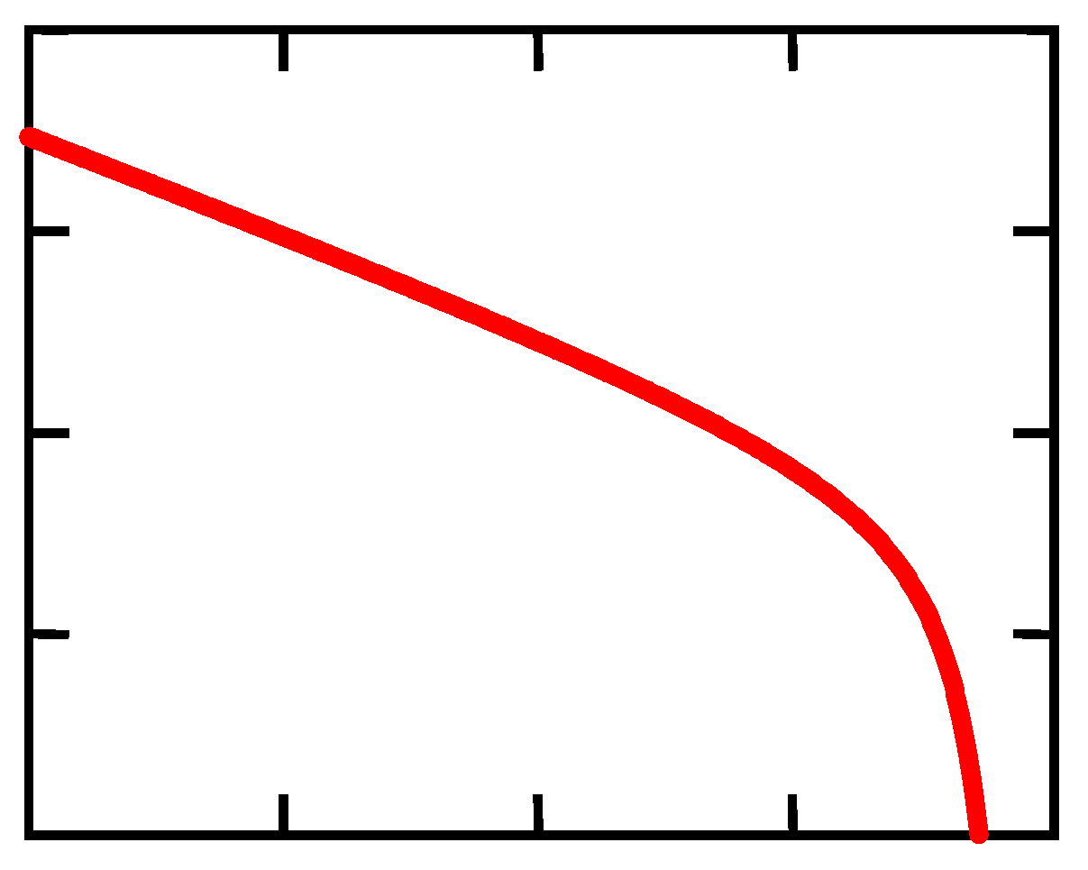
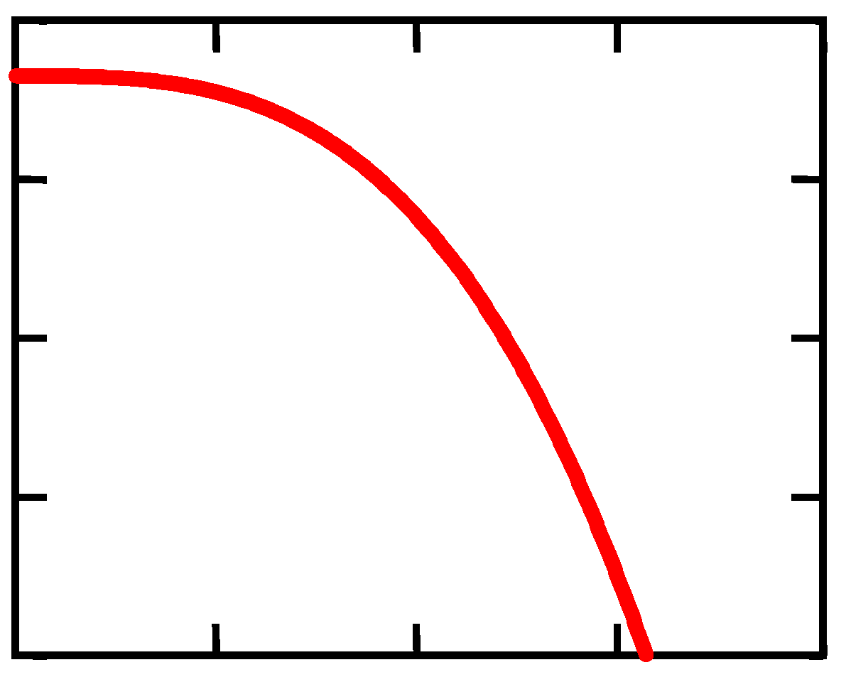
Figure 1. Voltaic pile design: Silvered copper (Ag), water (or washing soda solution), and zinc (Zn) or tin (Sn), and a metallic wire); (+) Zn(s) | Zn2+(aq) || H+(aq) | H2(g) (−), E 0.8 V .
Symmetry 15 00948 g001
Figure 2. Simplest model of a PV.
Symmetry 15 00948 g002
Figure 3. Single-diode model of a PV.
Symmetry 15 00948 g003
Figure 4. Double-diode model of a PV.
Symmetry 15 00948 g004
Figure 5. Potential vs. current for a PV.
Symmetry 15 00948 g005
Figure 6. Intensity vs. potential for a PV.
Symmetry 15 00948 g006
Figure 7. Vertical (“|”), horizontal (“−”), and perpendicular (“⊥”) offsets in calculating the experimental errors ( ϵ ).
Symmetry 15 00948 g007
Figure 8. Rational function f 1 ( x ) from Equation (2) with some convenient coefficients.
Symmetry 15 00948 g008
Figure 9. Power function f 2 ( x ) from Equation (3) with some convenient coefficients.
Symmetry 15 00948 g009
Figure 10. The simple circuit with a PV cell and a resistance used to collect the measurements.
Symmetry 15 00948 g010
Figure 11. Expressing the perpendicular offsets.
Symmetry 15 00948 g011
Figure 12. Evolution to optimum for f 1 from Equation (11).
Symmetry 15 00948 g012
Figure 13. Evolution to optimum for f 2 from Equation (12).
Symmetry 15 00948 g013
Table 1. Measured data for current intensity and potential in the simple circuit with PV cell.
I (mA)1.1471.1871.2571.3121.3621.4061.481.4931.5561.6091.6721.7421.7761.7851.8121.8211.834
U (mV)11321110108010381010973930900845772703593493405332254163
Table 2. Initial estimates for the coefficients.
n f ( x ; C ) Initial CStatisticsPV Cell Parameters
4 f 1 from Equation (11) a 1 = −3350
a 2 = 2689
a 3 = −476
a 4 = −1.93
R S S = 0.0015674
r adj 2 = 0.9976
F = 2396
I sc = 1.85482 mA
U oc = 1735.75 mV
I xp = 1.3921 mA
U xp = 982.02 mV
P xp = 1.3671 mW
3 f 2 from Equation (12) b 1 = 1.83
b 2 = −22
b 3 = 3.07
R S S = 0.0019093
r adj 2 = 0.9986
F = 9228
I sc = 1.83000 mA
U oc = 1576.51 mV
I xp = 1.3804 mA
U xp = 998.00 mV
P xp = 1.3776 mW
Table 3. Final optimized values for the coefficients.
n f ( x ; C ) Value CStatisticsPV Cell Parameters
4 f 1 from Equation (11) a 1 = −3349.81
a 2 = 2689.40
a 3 = −475.164
a 4 = −1.92823
R S S = 0.0013094
r adj 2 = 0.9977
F = 2526
I sc = 1.85071 mA
U oc = 1737.24 mV
I xp = 1.3866 mA
U xp = 985.94 mV
P xp = 1.3671 mW
3 f 2 from Equation (12) b 1 = 1.82622
b 2 = −22.2914
b 3 = 3.11345
R S S = 0.0011128
r adj 2 = 0.9987
F = 9528
I sc = 1.82622 mA
U oc = 1561.10 mV
I xp = 1.3823 mA
U xp = 991.19 mV
P xp = 1.3701 mW
Disclaimer/Publisher’s Note: The statements, opinions and data contained in all publications are solely those of the individual author(s) and contributor(s) and not of MDPI and/or the editor(s). MDPI and/or the editor(s) disclaim responsibility for any injury to people or property resulting from any ideas, methods, instructions or products referred to in the content.

